Abstract—Manual sorting of objects in an industrial environment is time consuming, labour intensive, unreliable and often impractical. This paper discusses the design and implementation of a decision making system that uses a support vector machine (SVM) as the main inference engine. The SVM driven sorting system is applied in an industrial environment for object classification and object placement. Object image vectors are compressed in order to reduce data dimensionality and only the pertinent feature vectors are extracted using the principle component algorithm. The SVM is trained with the feature vectors to classify the images. The performance of the SVM decision engine is evaluated with regards to its robustness and generalisation ability.
Index Terms—Support vector machine, separating hyperplane, image texture, sorting sytem
I. INTRODUCTION
ONE and texture are two important aspects of an image [1]. Image texture depends on its brightness and pixel locations [2] and its characteristics are displayed in the form of pixels. Pixel values and images can be identified by their texture [3]. Pixels are the basic elements of an image and contain its brightness value (color feature) and its shape and size information [2]. Techniques such as artificial intelligence are popular for image identification and yield good results. This paper discusses an alternate statistical approach, such as the support vector machine (SVM) to perform image identification. Image identification and classification with SVM’s is achieved by extracting key textural elements with image pre-processing methods such as wavelet compression (WC) and principle component
analysis (PCA), and then training the classifier to identify these salient characteristics. Supervised learning is used to train the SVM classifier to recognise
Manuscript received March 14, 2014; revised April 9, 2014. This work is supported in part by the National Research Foundation of South Africa and the Durban University of Technology.
P.Govender (corresponding author) is with the Optimisation and Energy Studies Group, Department of Electronic Engineering, Durban University of Technology, Durban, South Africa; Phone : +27 82 2991379; email: [email protected]
N.Pillay is with the Optimisation and Energy Studies Group, Department of Electronic Engineering, Durban University of Technology, Durban, South Africa; Phone : +27 84 6034586; email: [email protected]
the prescribed data. In this paper we will focus on the design
and the performance of the SVM for image identification under varying degrees of operational challenges. The paper is arranged as follows: Section 2 discusses the basic theory of SVM systems; Section 3 describes the steps followed to pre-process the data and create the target vectors. Section 4 discusses the steps followed to design the SVM decision engine.
II. BASIC THEORY OF THE SVM
SVM’s have been widely used for image identification [1]. A SVM is a statistical based pattern binary classification technique introduced by [4] and is based on the concept of structural risk minimization (SRM). A learning machine’s risk (R) is bound within the sum of the empirical risk (Rmp) and a confidence interval ψ i.e.
R
Rmp
[4]. A kernel function forms the main building block of a SVM and can be used with a wide range of different learning theories. The kernel function is used by the SVM to map a nonlinearly separable vector into a higher dimension space so as to make it linearly separable. A single SVM is a binary classifier for classifying two classes of data at any given time. The functionality of the SVM is extended by integrating several together to find solutions for multiclass data problems [5].A. The optimal separating hyperplane
The SVM algorithm is used to determine the optimal separating hyperplane between two classes of data. Assume dataset T has two separable classes and a total of k samples, where these samples are represented as (x1, y1), (x2, y2),…, (xk, yk). The class label is represented as
y
1
,
1
and is the binary value of two classes; nR
x
where nR
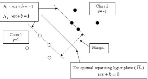
is an n-dimensional space.Consider the SVM in Fig. 1: Dataset T is separated into two classes by two parallel hyper-planes H1 and H2. Hyperplane H3 is the optimal separating hyperplane that lies parallel with
H
1andH
2and is equidistant between these two hyperplanes. H3 is defined asw
x
b
0
, where
denotes matrice multiplication, w is the normal vector to1
H
,H
2 and b represents the bias.Support Vector Machine Classification and
Sorting System for Cigarette Brands
Poobalan Govender, Member, IAENG and Nelendran Pillay
B. The Kernel function
The kernel function is the key component of the SVM classifier. Commonly used kernel functions include the polynomial function and the Gaussian and exponential radial basis functions. A kernel function locates the decision boundaries between different classes of data, making them linearly separable [6]. Binary class data being classified must meet the following condition:
k b wx y and k i b wx and k i b wx i i i i i i
i ( ) 1, 1,2....
1 1 , 1 1 1 , 1 (1)
From Fig. 1, the margin
||
||
2
w
m
is the absolutedistance between hyperplanes H1 and H2 [4]. This sets the restriction condition of the optimal separating hyperplane to ensure that m obtains its maximum value. We subject m to (1) and replaced it with its equivalent minimization of
2
||
||
2w
, which is then solved by the Lagrange formulation
(2):
y
wx
b
a
i
k
a
w
a
b
w
L
i k i i i ii
1
,
0
,
1
)
(
2
||
||
)
,
,
(
1 2 (2) wherea
i is the Lagrangian multiplier. To minimise L(w,b,a) we minimize w and b (3) :
k i k i i i i ii
b
a
y
b
L
and
y
x
a
w
w
L
1 10
0
,
0
(3)and maximise ai (4):
k i k i k j j i j i j ii
a
a
y
y
x
x
a
a
L
1 1 1
)
(
2
1
)
(
(4) for any i =1,….,n . The kernel (k) is defined by)
(
,
(
x
ix
jx
ix
jk
. The quadratic is subjected to (5):
k i i iy
a
10
, wherea
i
0
i
1
,...
k
(5)
The construction of the optimal separating hyperplane depends on solving the quadratic programming problem with (4) and (5). The SVM classifier is defined in (6):
0 , 1sgn
sgn(
)
(
ab
x
x
a
y
b
x
w
x
f
i i i(6)
III. IMAGE PRE-PROCESSING AND TARGET VECTORS
A. Image Pre-processing
Image pre-processing involves image capture, image compression and feature extraction. The images considered for this study are given in Fig. 2. The identification of these images is performed with the SVM, and its ability to generalize and remain robust in spite of noise was also assessed.
Image compression: Image compression is achieved with the Haar wavelet (HW). HW decomposes a signal into a summation of a series of baby wavelets that are generated through dilating and shifting operations from a mother wavelet [7]. HW compression is chosen over other traditional compression methods because it provides a multi-resolution representation of an image and also yields a higher compression ratio [1], [8].
Principal component analysis (PCA): The HW compressed data is subjected to PCA in order to reduce the dataset for easing computation burden [9]. PCA retains the unique characteristic feature vectors which contribute most to the variance of the image under consideration by determining the eigenvectors and the eigenvalues of the covariance matrix. Each column of the eigenvector matrix with the highest eigenvalues consists of the principal components and forms the feature vector set.
B. Creating Training Vectors
A comprehensive set of image vectors for object is determined as follows:
[image:2.595.308.554.55.187.2]i) 3 images of each box from 1200, 2400 and 3600 orientations are captured of each box when the box is in
[image:2.595.309.560.230.315.2]a first pose. The 3 images of the respective box in its first pose are clustered together to form a group. ii)The pose of each box is adjusted 5 times and 3 images are
taken of the box in each respective pose. From this we will have 5 groups of images, with each group having three images of the same box positioned in a 1200, 2400 and 3600 pose.
iii) Repeat (i) and (ii) for each box. This results in a total of 15 groups of vectors (5 for each box), with each group having three images of each object occupying a specific pose. These image vectors have different position orientations and poses to ensure that accurate recognition will always take place even within an environment experiencing varying conditions. Following HWT compression of the object image in each of its poses, PCA is applied to the compressed image in order to extract the feature vectors, a sample of which is given in Table 1. These vectors are used to train the SVM.
The above procedure was heuristically developed and yielded a comprehensive collection of image vectors for each box. These vectors captured the tone and textural characteristics for each box in different positional orientations and poses, and ensured that accurate recognition always occurred even under dynamic environmental conditions.
IV. SVMDECISIONENGINE
SVM’s are binary classifiers and are extensively applied to empirical classification operations [10]. For this study, the SVM was taught to discriminate between different brands of cigarette boxes. A SVM was trained to utilise a hyperplane to separate one set of similar data features from another [11]. The subsets of data vectors within each grouping of similar data are known as the support vectors [12]. The images in Fig. 2 are used to create the three data classes for this study. Because the SVM classifier can only classify two different data samples at a time, we converted our multi-class multi-classification problem into two binary multi-class problems and designed and trained a multi-level two SVM system to classify the three image types. Fig. 3 illustrates the multi-level SVM decision making tree system used in the study. The test sample on Level 1 has three data classes which correspond to the Aspen, Lucky-Strike and Winfield carton images, respectively. At Level 1 the SVM is trained to recognize the Aspen-Lucky-Strike vector combination as the one group and the Winfield vectors as the other group. At
Level 2 the SVM is trained to separate the Lucky-Strike carton from the Aspen carton.
SVM performance depends largely on the selected kernel
function, which is one of the main weaknesses of this technique [13]. Proper selection of the kernel function determines how well the SVM generalizes [6]. Since there is no rigid technique for choosing a specific kernel function, we followed an iterative process to select an appropriate function. A linear kernel function was chosen based on its performance for the Level 1 and Level 2 SVM classifiers.
A. Layout and Operation
Fig. 4 shows the SVM based classification and sorting system. The work environment consists of three 0.3 megapixel cameras situated 1200 apart that capture up to 30 frames per second, a robot controller (slave) and manipulator arm, plus a robot control computer (master). The 3 cameras simultaneously capture each box image from 3 different angles for the creation of a comprehensive image matrix. Communication between each camera and the robot control computer is done via the 3 universal serial bus ports, and occurs at a maximum data transfer rate of 480 Mega-bytes per second.
The slave robot controller module receives control signals from the master robot control computer. The slave controls the gripper, plus the vertical motion and angular rotation of the manipulator. The purposes of the slave controller is to receive and pre-process image data, transmit PCA data to the remote master computer, receive control signals from the master and guide the robot arm to a pre-allocated position for each work-piece. The main master computer was housed in a control room situated 10m from the work environment and was used to receive PCA feature vectors from the remote slave controller, recognise images using the SVM recognition system and transmit the object recognition signal to the slave robot controller. The operation of the object classification system in Fig. 4 is as follows:
At rest the robot arm will idle at its default position. During the sorting operation images of the unsorted objects are captured and pre-processed by the robot control computer using wavelet image compression and PCA. The
Fig. 3. Multiclass SVM decision engine.
TABLEI
selected feature vectors are transmitted via the Bluetooth link to the master control computer for classification by the SVM system. After classification a control signal is transmitted via Bluetooth to the remote slave controller. The slave controller guides the robot to pick the objects from ‘unsorted object positions 1, 2 and 3’ and relocate them to ‘sorted object positions 1, 2 and 3’. This sequence of operations continues till all objects have been sorted and stacked into their respective locations. The arm returns to its default resting position following a ‘pick and place’ operation.
V. SVMPERFORMANCE
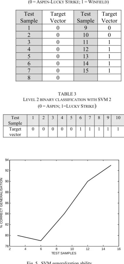
Table 2 shows the results of the SVM1 classifier. The 0 denotes the target vectors of the Aspen-Lucky Strike combination and 1 denotes the Winfield carton target vectors. On Level 2, the SVM2 classifier differentiates between the Aspen and Lucky Strike cartons. In Table 3 for the SVM2 classifier, the 0 denotes the Aspen carton and the 1 represents the Lucky Strike carton. From these results we can conclude that the three different boxes were recognized successfully with a recognition rate of 100%.
Fig. 5 shows the results of the test conducted to assess the ability of the SVM to generalise. Image data was used as training data for the SVM classifier. We used five SVM classifiers to test for generalization. These were trained using 3, 6, 9, 12 and 15 samples respectively for each cigarette box, and each test sample had 20 images of a cigarette box. From Fig. 5, we see an improvement in the SVM’s ability to generalise.
The SVM was also tested for robustness against
environmental noise and the results are shown in Fig. 6. Artificial ‘salt and pepper’ noise was used to test the immunity of the SVM classifiers to noise interferences. Varying degrees of noise was applied to 15 test samples to assess the robustness of the SVM classifier. From Fig. 6, we observe the following: For small quantities of data and low noise levels the SVM’s performance is relatively robust, but its performance deteriorated when the noise level was increased.
TABLE2
LEVEL 1 BINARY CLASSIFICATION WITH SVM1 (0=ASPEN-LUCKY STRIKE;1=WINFIELD)
Test
Sample Vector Target Sample Test Vector Target 1 0 9 0 2 0 10 0 3 0 11 1 4 0 12 1 5 0 13 1 6 0 14 1 7 0 15 1 8 0
Fig. 4. SVM classifier and sorter system operating environment.
TABLE3
LEVEL 2 BINARY CLASSIFICATION WITH SVM2 (0=ASPEN;1=LUCKY STRIKE)
Test Sample
1 2 3 4 5 6 7 8 9 10 Target
vector
0 0 0 0 0 1 1 1 1 1
2 4 6 8 10 12 14 16 30
35 40 45 50 55 60 65
TEST SAMPLES
%
C
O
R
R
EC
T
C
L
ASS
IF
IC
AT
IO
N
0.2 noise level 0.4 noise level
Fig. 6. SVM classification for varying noise levels.
2 4 6 8 10 12 14 16 78
80 82 84 86 88 90 92 94
TEST SAMPLES
%
CO
RR
E
CT
G
E
N
E
RA
L
IS
A
T
IO
[image:4.595.42.292.43.207.2]N
[image:4.595.331.543.62.513.2]VI. SUMMARY AND CONCLUSION
The paper has described the design of an image classification system that uses SVM to perform image classification. The binary classification structure of the SVM
is extended by fusing multiple SVM’s in order to classify multiple classes of data. To minimize computation burden, the dimensionality of image data is reduced with the HWT and PCA. This reduced dataset with the salient feature vectors is applied to the SVM classification engine. The performance of the SVM was also assessed with respect to its ability to generalise and classify within a noisy environment. This was done in order to reproduce as closely as possible a real world industrial environment where this type of classification and sorting system is applied. From the results, we observed that the SVM’s ability to generalise improved as the data increased (cf. Fig. 5). With regards to robustness (cf. Fig.6), SVM performance deteriorates significantly as noise level and data increases. The overall performance of the SVM is satisfactory, but a better choice for a classification system would be the artificial neural network as they are simpler and easier to train and generally yield excellent results when properly designed and trained [14].
REFERENCES
[1] M. Seetha, I.V Muralikrishna, B.L Deekshatulu, B.L Malleswari, Nagaratna, and P. Hegde, “Artificial neural networks and other methods of image classification,” Journal of Theoretical and Applied Information Technology, 2005-2008, pp. 1039-1053.
[2] D.Wua, H.Yang , X. Chen,Y. He, X. Li, “Application of image texture for the sorting of tea categories using multi-spectral imaging technique and support vector machine,” Journal of Food Engineering (88), 2008, pp. 474–483.
[3] C.H. Chen, L.F. Pau and P.S. Wang P.S., “Handbook of pattern recognition and computer vision,” World Scientific, 1993.
[4] V.N. Vapnik, “The nature of statistical learning,” Springer-Verlag, 1995.
[5] A. David and B. Lerner, “Support vector machine-based image classification for genetic syndrome diagnosis,” Pattern Recognition Letters (26), 2004-2005, pp. 1029– 1038.
[6] N. Cristianini and J. Shawe-Tayler. “An introduction to support vector machines and other kernel-based learning methods,” Cambridge University Press, 2000. [7] H. Zhang, C.M. Cartwright, M.S. Ding and W.A
Gillespie, “Image feature extraction with various wavelet functions in a photorefractive joint transform correlator,” Transactions on Optic Communications 185, 2000, pp. 277-284, Elsevier Science.
[8] P. Raviraj and M.Y. Sanavullah, “The modified 2D Haar wavelet transformation in image compression,” Middle East Journal of Scientific Research” 2(2), 2007, pp. 73-78.
[9] M.S. Nixon and A.S. Aguado, “Feature Extraction and Image Processing,”Academic Press, 2008.
[10] S. Nashata, A. Abdullahb, S. Aramvithc and M.Z. Abdullaha, “Support vector machine approach to real-time inspection of biscuits on moving conveyor belt,” Computers and Electronics in Agriculture (75), 2011, pp. 147–158.
[11] N. Razmjooya, B. S. Mousavib, F. Soleymani, “A real-time mathematical computer method for potato inspection using machine vision,” Computers and Mathematics with Applications (63), 2012, pp. 268– 279.
[12] Z.-M. Yanga, J.-Y. Heb,Y.-H. Shaoa,” Feature Selection Based On Linear Twin Support Vector Machines”, Procedia Computer Science (17), 2013, pp. 1039 – 1046.
[13] C.J.C. Burges, “A tutorial on support vector machines,” 1998, Kluwer academic publishers.