Statistical Analysis of BRDF Data for Computer
Graphics and Metrology
Mikhail Langovoy, Gerd W¨ubbeler, and Clemens Elster
Abstract—Characterizing the appearance of real-world sur-faces is a fundamental problem in multidimensional reflec-tometry, computer vision and computer graphics. For many applications, appearance is sufficiently well characterized by the bidirectional reflectance distribution function. BRDF is one of the fundamental concepts in such diverse fields as multidimen-sional reflectometry, computer graphics and computer vision. In this paper, we treat BRDF measurements as samples of points from high-dimensional non-linear non-convex manifold. We argue that statistical data analysis of BRDF measurements has to account both for nonlinear structure of the data as well as for ill-behaved noise. Standard statistical methods can not be safely directly applied to BRDF data. Our study clarifies certain pitfalls in analysis of BRDF data, and helps to develop more refined estimates and unsupervised learning procedures for BRDF models. We also apply the notion of Pitman closeness to compare different estimators and learning procedures for BRDF models. This criterion for comparison is loss function-free and seems to be especially appropriate for applications in metrology and in comparing different types of learning methods. Additionally, we outline a multiple testing procedure for testing a hypothesis that a material has diffuse reflection in a generalized sense.
Index Terms—BRDF, computer graphics, metrology, data analysis, statistics of manifolds.
I. INTRODUCTION
C
HARACTERIZING the appearance of real-world sur-faces is a fundamental problem in multidimensional reflectometry, computer vision and computer graphics. For many applications, appearance is sufficiently well charac-terized by the bidirectional reflectance distribution function (BRDF).In the case of a fixed wavelength, BRDF describes re-flected light as a four-dimensional function of incoming and outgoing light directions. In a special case of rotational symmetry, isotropic BRDFs are are used. Isotropic BRDFs are functions of only three angles. The BRDF is applied under the assumption that all light falls at a single surface point. The classical device for measuring BRDFs is the gonio-reflectometer, which is composed of a photometer and light source that are moved relative to a surface sample under computer control.
In computer graphics and computer vision, usually either physically inspired analytic reflectance models [1], [2], [3], or parametric reflectance models chosen via qualitative crite-ria [4], [5], [6], [7] are used to model BRDFs. These BRDF models are only crude approximations of the reflectance
Manuscript received July 8, 2014; revised August 15, 2014. This work has been carried out within EMRP project IND 52 ’Multidimensional reflectometry for industry’. The EMRP is jointly funded by the EMRP participating countries within EURAMET and the European Union.
M. Langovoy is with the Physikalisch-Technische Bundesanstalt, Berlin, 10587 Germany e-mail: [email protected] .
G. W¨ubbeler and C. Elster are with the Physikalisch-Technische Bunde-sanstalt, Berlin, 10587 Germany.
of real materials. Moreover, analytic reflectance models are limited to describing only special subclasses of materials.
In multidimensional reflectometry, an alternative approach is usually taken. One directly measures values of the BRDF for different combinations of the incoming and outgoing angles and then fits the measured data to a selected ana-lytic model using optimization techniques. There are several shortcomings to this approach as well.
In computer graphics, it is important that BRDF mod-els should be processed in real-time. Computer-modelled materials have to remind real materials qualitatively, but quantitative accuracy is not as important. The picture in reflectometry and metrology is almost the opposite: there is typically no need in real-time processing of BRDFs, but quantitative accuracy is the paramount. In view of this, some of the breakthrough results from computer vision and animation would not fit applications in reflectometry and in many industries.
Another difference with virtual reality models is that in computer graphics measurement uncertainties are essentially never present. This is not the case in metrology, reflectometry and in any real-world based industry [8]. Since measurement errors can greatly influence shape and properties of BRDF manifolds, there is a clear need to develop new methods for handling BRDFs with measurement uncertainties.
In this paper, we treat BRDF measurements as samples of points from a high-dimensional and highly non-linear non-convex manifold. We argue that any realistic statistical analysis of BRDF measurements has to account both for nonlinear structure of the data as well as for a very ill-behaved noise. Standard statistical methods can not be safely directly applied to BRDF data. Our study of parameters for generalized Lambertian models clarifies certain pitfalls in analysis of BRDF data, and helps to understand and develop more refined estimates for more realistic BRDF models that will be studied in subsequent papers. Second, we would use the generalized Lambertian model parameter estimators from Section 6 to build statistical tests to test a hypothesis whether any particular material is diffuse or not.
II. MAIN DEFINITION
The bidirectional reflectance distribution function (BRDF), fr(ωi, ωr))is a four-dimensional function that defines how light is reflected at an opaque surface. The function takes a negative incoming light direction,ωi, and outgoing direction, ωr, both defined with respect to the surface normal n, and returns the ratio of reflected radiance exiting along ωr to the irradiance incident on the surface from direction ωi. Each direction ω is itself parameterized by azimuth angle φ and zenith angleθ, therefore the BRDF as a whole is 4-dimensional. The BRDF has unitssr−1, with steradians (sr)
being a unit of solid angle.
The BRDF was first defined by Nicodemus in [9]. The definition is:
fr(ωi, ωr) =
d Lr(ωr) d Ei(ωi)
= d Lr(ωr)
Li(ωi) cosθid ωi . (1)
where L is radiance, or power per unit solid-angle-in-the-direction-of-a-ray per unit projected-area-perpendicular-to-the-ray, E is irradiance, or power per unit surface area, and θi is the angle between ωi and the surface normal,n. The indexiindicates incident light, whereas the indexrindicates reflected light.
III. IMPORTANT MODELS OF DIFFUSE REFLECTION A. Lambertian model
Lambertian model [4] represents reflection of perfectly diffuse surfaces by a constant BRDF. Because of its sim-plicity, Lambertian model is extensively used as one of the building blocks for models in computer graphics. It was believed for a long time that the so-called standard diffuse reflection materials exhibit Lambertian reflectance, but recent studies with actual BRDF measurements convincingly reject this hypothesis [10], [11], [12].
B. Oren-Nayar model
Oren-Nayar model [1] is a ”directed–diffuse” microfacet model, with perfectly diffuse (rather than specular) micro-facets. It can be viewed as a generalization of the Lambertian model. This is a reflectance model for diffuse reflection from rough surfaces. Oren-Nayar model is typically used to predict the appearance of rough surfaces, such as concrete or sand. Resently, a more sophisticated model was proposed by [13]. This new model includes as special cases both Lam-bertian model and the Oren–Nayar model, as well as the Torrance–Sparrow model with specular microfacets.
C. Lommel-Seeliger
Lommel-Seeliger model [14] is used to simulate the brightening of a rough surface when illuminated from di-rectly behind the observer. This is a physically inspired model of a special class of reflections from diffuse surfaces. This model is typically applied to model astronomical data, such as lunar and Martian reflection.
IV. STATISTICAL ANALYSIS OFBRDFMODELS
In this section, we treat parameter estimation for BRDF models of standard diffuse reference materials. These materi-als are supposed to have ideal diffuse reflection with constant BRDFs. Graphically, for each incoming anlge θi, ϕi, the resulting BRDFfr(ωi, ωr)is a (subset of) two-dimensional upper hemisphere. The radius ρ of this hemisphere is the parameter that we aim to estimate in this paper.
As we mentioned before, the Lambertian model has been shown to be inaccurate even for those materials that were designed to be as close to perfectly diffuse as possible. Therefore, parameter estimates determined for the Lamber-tian model can hardly be used in practice. However, there are two methodological reasons that make these estimators worth a separate study.
First, BRDF measurements represent a sample of points from a high-dimensional and highly non-linear non-convex manifold. Moreover, these measurements are collected via a nontrivial process, possibly involving random or systematic measurement errors of digital or geometric nature. These two observations suggest that any realistic statistical analysis of BRDF measurements has to account both for nonlinear structure of the data as well as for a very ill-behaved noise. Standard statistical methods typically assume nice situations like i.i.d. normal errors, and can not be safely directly applied to BRDF data. Our study of parameters for Lambertian models clarifies certain pitfalls in analysis of BRDF data, and helps to understand and develop more refined estimates for more realistic BRDF models that will be studied in subsequent papers.
Second, we would use the Lambertian model parameter es-timators to build statistical tests to test a hypothesis whether any particular material is perfect diffuse or not. This will be studied in a separate paper.
Suppose we have measurements of a BRDF available for theset of incoming angles
Ωinc =
ωi(p) Pinc
p=1 =
θ(ip), ϕ(ip) Pinc
p=1 . (2)
HerePinc≥1is the total number of incoming angles where the measurements were taken. Say that for an incoming angle
ω(ip) we have measurements available for angles from the
set of reflection angles
Ωref l = Pinc
[
p=1
Ωref l(p), (3)
where
Ωref l(p) =
ω(rq)
Pref l(p)
q=1
=
θ(rq), ϕ(rq)
Pref l(p)
q=1
,
where
Pref l(p) Pinc
p=1 are (possibly different) numbers of
measurements taken for corresponding incoming angles. Overall, we have the set of random observations
f θi(p), ϕ(ip), θr(q), ϕ(rq) θ
(p)
i , ϕ
(p)
i
∈Ωinc,
θr(q), ϕr(q)∈Ωref l(p)
Our aim is to infer properties of the BRDF funtion (1) from the set of observations (4). In general, the connection between the true BRDF and its measurements is described via a stochastic transformationT, i.e.
f(ωi, ωr) = T fr(ωi, ωr)
, (4)
where
T : M × P × F4 → F4, (5)
with M = (M,A, µ) is an (unknown) measurable space, P = (Π,P,P) is an unknown probability space, F4 is
the space of all Helmholtz-invariant energy preserving 4-dimensional BRDFs, and F4 is the set of all functions of
4 arguments on the 3-dimensional unit sphereS3 inR4.
Equations (4) and (5) mean that there could be errors of both stochastic or non-stochastic origin. In this setting, the problem of inferring the BRDF can be seen as a statistical inverse problem. However, contrary to much literature on this subject, we do not assume linearity of the transformationT, we do not assume that T is purely stochastic, and we do not assume an additive model with zero-mean parametric errors, as these assumptions do not seem realistic for BRDF measurements.
Of course, this setup is intractable in full generality, but for special cases such as inference for Lambertian model, we would be able to obtain quite general solutions.
It is also easily observable (see, e.g., [10]) that for all materials their sub-BRDFs, consisting of measurements for different incoming angles, look substantially different (no matter if we believe in the underlying Lambertian model or not). This suggests that different sub-BRDFs of the same material still have different parameter values, and this in turn calls for applying statistical procedures separately for different sub-BRDFs and for combining the results via model selection, multitesting and related techniques.
V. MEANS,MEDIANS AND ROBUST ESTIMATORS A. Basic properties of distributions in BRDF data
In our choice of estimators for parameters in BRDF models, we have to take into account specific properties of BRDF data. It is important to notice that, due to the complicated structure of measurement devices, outliers are possible in the data. Additionally, due to technical difficulties in measuring peak values of BRDFs (see [15], [16]), we have to count on the fact that certain (even though small) parts of the data contain observations with big errors. This also leads us to conclusion that, even for simplest additive error models, we cannot blindly assume that random errors are identically distributed throughout the whole manifold. Additionally, missing data are possible and even inevitable for certain angles. Measurement angles themselves can be also arbitrary and non-uniformly distributed.
In view of the above arguments, a useful estimator for any BRDF model has to exhibit certain robustness against outliers and dependent or mixed errors.
An estimator has to be universal enough in the sense that it has to be applicable to BRDF samples without requiring extra regularity in the data set, such as uniformly distributed (or other pre-specified) design points, pre-specified large number
of measurements, or absence of missing values. This obser-vation suggests that simpler estimators are more practical for BRDF data than complicated (even if possibly asymptotically optimal) estimators, as the later class of estimators has to rely on rather strict regularity assumptions about the underlying model.
B. Pitman closeness of estimators
Let Ω be a probability space and let θb1 : Ω → R and b
θ2 : Ω → R be estimators of a parameter θ ∈ R. Then
thePitman relative closenessof these two estimators at the pointθis defined as
P θb1,bθ2;θ = P
bθ1−θ
<
bθ2−θ
. (6)
The estimatorθb1 isPitman closer toθthanθb2, if
P θb1,bθ2;θ > 1/2.
While this criterion for comparison of estimators is much less known as, say, unbiasedness or asymptotic variance, it appeals to the actually observable precision of estimators, and thus seems of interest for applications in metrology.
We apply the notion of Pitman closeness to compare different estimators that could be used in BRDF models. Based on this and other criteria, we show that, in the context of BRDF model parameter estimation, estimators based on either median or trimmed mean are safer to use and are often more accurate than estimators based on sample means.
We refer to [17] for an extensive discussion of the relative closeness of estimators and other related notions and their properties. Besides unbiasedness, asymptotic variance and relative closeness, there are many other criteria for comparing quality of statistical estimators. At least 7 of them can be found in [18].
C. Definitions of basic estimators
To exemplify these arguments, we consider the following basic estimators for the radius parameter of the Lambertian model: sample mean; sample median; trimmed (truncated) mean.
LetX1, X2, . . . , Xn be a sample from probability distri-butionF. Then thesample meanis defined as
sm(X) = 1
n n
X
i=1
Xi. (7)
LetX(1) ≤X(2) ≤. . . ≤X(n) be the order statistics of
the sample X1, X2, . . . , Xn. Thesample median is defined as
smed(X) =
X((n+1)/2), n is odd;
1
2 X(n/2)+X(n/2+1)
, n is even.
Let 0 ≤ α < 1/2 be a number, and let [·] denote the integer part of a real number. Then thesample trimmed mean
tmα(X) =
1
n(1−2α)
n−[nα]−1 X
i=[nα]+2
X(i) +
([nα] + 1−nα) X([nα]+1)+X(n−[nα])
.
If Fn denotes the empirical distribution function of the sample X1, X2, . . . , Xn, then we can write, equivalently,
tmα(X) =
1 1−2α
Z 1−α
α
Fn−1(t)dt . (8)
D. Mean and median
Sample mean is known to be an asymptotically efficient estimator, as well as a uniformly minimum-variance unbiased estimator, for the expected value of the random variable. However, it is important to note that these nice properties are guaranteed only for sufficiently ”nice” distributions (see [19] or [20]), while sometimes even marginal deviations from these nice models seriously spoil performance of the sample mean estimator. Even if the regularity conditions are only slightly violated, the sample mean estimator can lose its efficiency or can become inconsistent.
In view of the above discussion of properties of BRDF data, we conclude that it is not advisable to apply the sample mean directly as an estimator of the Lambertian radius.
Here we bring some examples to illustrate our points. An example from pp. 2 - 5 of [21] shows that, while the sample mean is even finite sample efficient for estimating parameters of normal distribution, this estimator loses its nice performance properties already for mixtures of two normal distributions. Moreover, even a mixture with 0.2 percent of a different normal distribution can cause the sample mean to lose its efficiency.
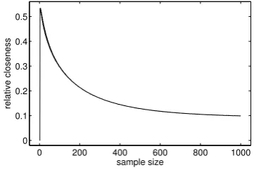
In this and in the next subsection, we present some results of an extensive Monte Carlo experiment comparing relative closeness of different types of basic nonparametric estimators. Each of the graphs contains values of relative closeness obtained for samples of all sizes ranging from 1 to 1000 observations. We performed 1000000 comparisons for each sample size.
Figure 1 shows that for a sample of i.i.d. normal random variables mean has better relative closeness than the median, with the actual value being above 0.6. We notice that the situation remains essentially the same regardless of the variance of the underlying normal distribution.
However, if we are dealing with a heavy-tailed distribution, the picture changes. Suppose we are presented with a Cauchy distribution, and our goal is to estimate the mode (the mean does not exist in this case). Then Figure 2 shows that the relative closeness of the mean tends to 0 when compared with the median.
Mean surprisingly loses its efficiency even in rather smooth toy situations. Suppose that a sample from i.i.d. standard normal distribution is contaminated with 5% of i.i.d. normals with mean 0 and variance 10. The result is shown on Figure 3. Mean’s closeness compared to median drops to 0.3. Even more surprisingly, if we start with a sample of i.i.d. normals with mean 0 and variance 100 and contaminate this sample with just 5% of i.i.d. normals with mean 0 and small
0 200 400 600 800 1000
0 0.1 0.2 0.3 0.4 0.5 0.6
sample size
[image:4.595.335.517.52.173.2]relative closeness
Fig. 1. Mean beats median for the standard normal distribution
0 200 400 600 800 1000
0 0.05 0.1 0.15 0.2 0.25 0.3 0.35
sample size
[image:4.595.338.517.205.320.2]relative closeness
Fig. 2. Median grossly outperforms mean for heavy-tailed distributions
0 200 400 600 800 1000
0 0.1 0.2 0.3 0.4 0.5
sample size
relative closeness
Fig. 3. Median can outperform mean for mixtures of normal distributions
0 200 400 600 800 1000
0 0.1 0.2 0.3 0.4 0.5
sample size
relative closeness
Fig. 4. Median can outperform mean for mixtures of normal distributions with small errors
variance 1, the drop in mean’s closeness compared to median is even worse. Figure 4 shows that the relative closeness of mean drops to 0.1.
E. Truncated mean and mean
[image:4.595.336.516.353.475.2] [image:4.595.336.517.505.626.2]0 200 400 600 800 1000 0
0.05 0.1 0.15
sample size
[image:5.595.83.266.53.172.2]relative closeness
Fig. 5. Trimmed mean totally dominates mean for Cauchy distributions
in the sense of both Pitman closeness, as well as asymptotic relative efficiency.
The picture can be reversed when our data are allowed to contain outliers or when the data can be, at least partially, generated by a heavy-tailed distribution (which is the case when large values of measurement errors are possible, as is the case for BRDF measurements of specular peaks). We give here a toy example with a Cauchy distribution. Figure 5 illustrates the relative efficiency of mean compared to the trimmed mean with 10% of the extremes in data being discarded. The unusual shape of the relative closeness curve has no explanation at the moment.
Here the mean is an inconsistent estimator of the median of the distribution, while the truncated mean is not only a consistent estimator of the median, but, with a proper choice of the truncation point, is capable of outperforming the sample median in estimating the median [22]! One needs to drop out about 76% of the data, though. In fact, even more efficient estimators exist [23], but they require to drop out almost all of the data, and we would not advise to use them for estimation in BRDF models or for any work with moderate sample sizes.
VI. PARAMETER ESTIMATION FOR GENERALIZED
LAMBERTIAN MODELS
For each ωi(p) from the set of incoming angles Ωinc, let ρ(p)denote the Lambertian radius of the BRDF’s layer
f θ(ip), ϕ(ip), θ(rq), ϕ(rq) θr(q), ϕ(rq)
∈Ωref l(p)
, (9)
where Ωref l(p) is defined by (3). Thus, we are estimating the Pinc-dimensional parameter vector
ρ(p)
Pinc
p=1
. (10)
For1≤p≤Pinc, let
f((ip))
Pref l(p)
i=1
(11)
be the non-decreasing sequence of order statistics of the subsample (9). Then the sample median estimator of the parameter vector (10) is defined as
\
smed(p)
Pinc
p=1
, (12)
where
\
smed(p)(f) =
f(((pP)
ref l(p)+1)/2), ifPref l(p)is odd;
1 2 f
(p)
(Pref l(p)/2)+f
(p)
(Pref l(p)/2+1)
,
ifPref l(p)is even.
Let 0 ≤ α < 1/2 be a number, and let [·] denote the integer part of a real number. Then thesample trimmed mean
estimator of the parameter vector (10) is defined as
[
tm(αp)
Pinc
p=1
, (13)
where
[
tm(αp)(f) =
1
Pref l(p)(1−2α)
×
[Pref l(p)α] + 1−Pref l(p)α
f([(pP)
ref l(p)α]+1)+
f((Pp)
ref l(p)−[Pref l(p)α])
+
Pref l(p)−[Pref l(p)α]−1 X
i=[Pref l(p)α]+2
f((ip))
.
VII. HYPOTHESIS TESTING FOR GENERALIZED DIFFUSE REFLECTION MODELS
It is rather straightforward to build a test for checking whether any particular material is perfectly diffuse. Indeed, the corresponding null hypothesis can be tested via a t -statistic on the basis of the observed set of BRDF values. However, as we noted above, testing this hypothesis is not very informative as this null hypothesis will be rejected even for those materials that serve as diffuse reflectance standards. Therefore, it makes more sense to test a hypothesis that a material has diffuse reflection in general, even though not perfectly diffuse with the same level of reflection for each incoming angle. This amounts to building a multiple testing procedure for testing the joint hypothesis H0 =
T
1≤p≤PincHp, whereHp is thep-th null hypothesis stating
that thep-th layer (9) is laying on a sphere.
As an application of the above estimators, we construct now a test for H0. For simplicity of notation, we use
the median-based estimator. Consider the sequence of test statistics{M Tp}1≤p≤Pinc, where
M Tp =
√
n
SSD(p)× (14)
1
Ωref l(p)
X
θr(q),ϕ(q)r
∈Ωref l(p)
f θi(p), ϕ(ip), θr(q), ϕ(rq)
−minsmed\(p),1/π
!
fact, M Tp is best suited for testing a hypothesis that the points of the true p−th layer of the BRDF belong to a sphere, while they were measured with normally distributed independent errors, versus the alternative that the points of the p−th layer are not symmetric about the median and tend to have bigger deviations from the median. We also introduced the1/π-correction in (14) in order to account for the energy conservation law, as we are only interested in testing against physically plausible alternatives. Depending on the assumptions that we make about measurement errors, it is possible to use any other appropriate test statistics instead of {M Tp}1≤p≤Pinc. The principle of constructing
the multiple test remains the same.
Let us apply the standard test based onM Tpfor testing the hypothesisHp for allp. Denote the corresponding resulting p-values by P V1, . . . , P VPinc, and let P V(1) ≤ . . . ≤
P V(Pinc)be the ordered set of thesep-values. Then one could
suggest to reject H0 ifP V(p)≤pα/Pinc for at least onep. Under certain conditions, this multiple testing procedure is asymptotically consistent and more powerful than the procedure based on the Bonferroni principle. See [24] for details related to rigorous analysis of this type of multiple testing methods.
Note that it is crucial to take into account the multi-plicity of tests. Otherwise, irrespectively of what kind of test statistics we use, if the decisions about each of the basic hypothesis H0, . . . , HPinc are made on the basis of
the unadjusted marginal p−values, then the probability to reject some true null hypothesis will be too large and the test will not be reliable. Unfortunately, this mistake is commonly made in applications of multiple testing.
VIII. CONCLUSION
BRDF is one of the fundamental concepts in such diverse fields as multidimensional reflectometry, computer graphics and computer vision. Most of BRDF models are only crude approximations of reflectance of real materials. In view of this, some of the breakthrough results from computer vision and animation would not fit applications in reflectometry and in many industries.
In this paper, we treated BRDF measurements as sam-ples of points from high-dimensional non-linear non-convex manifold. We have shown that statistical analysis of BRDF measurements has to account both for nonlinear structure of the data as well as for ill-behaved noise. Standard statistical methods can not be safely directly applied to BRDF data. Our study of parameters for Lambertian models clarified certain pitfalls in analysis of BRDF data. We developed more refined estimators for BRDF models of standard diffuse reference materials.
We also applied the notion of Pitman closeness to compare different estimators for BRDF models. This criterion for comparison of estimators seems to be especially appropri-ate for applications in metrology. Based on this and other criteria, we have shown that, in the context of BRDF model parameter estimation, estimators based on either median or trimmed mean are safer to use and are often more precise than estimators based on sample means. Additionally, we outlined a multiple testing procedure for testing a hypothesis that a material has diffuse reflection in a generalized sense.
REFERENCES
[1] M. Oren and S. K. Nayar, “Generalization of the lambertian model and implications for machine vision,”International Journal of Computer Vision, vol. 14, no. 3, pp. 227–251, 1995.
[2] R. L. Cook and K. E. Torrance, “A reflectance model for computer graphics,” inACM Siggraph Computer Graphics, vol. 15, no. 3. ACM, 1981, pp. 307–316.
[3] X. D. He, K. E. Torrance, F. X. Sillion, and D. P. Greenberg, “A com-prehensive physical model for light reflection,” inACM SIGGRAPH Computer Graphics, vol. 25, no. 4. ACM, 1991, pp. 175–186. [4] J. Lambert and E. Anding,Lamberts Photometrie: (Photometria, sive
De mensura et gradibus luminis, colorum et umbrae) (1760), ser. Ostwalds Klassiker der exakten Wissenschaften. W. Engelmann, 1892, no. v. 1-2. [Online]. Available: http://books.google.de/books? id=Fq4RAAAAYAAJ
[5] B. T. Phong, “Illumination for computer generated pictures,”Commun. ACM, vol. 18, no. 6, pp. 311–317, Jun. 1975. [Online]. Available: http://doi.acm.org/10.1145/360825.360839
[6] J. F. Blinn, “Models of light reflection for computer synthesized pictures,” inProceedings of the 4th annual conference on Computer graphics and interactive techniques, ser. SIGGRAPH ’77. New York, NY, USA: ACM, 1977, pp. 192–198.
[7] E. P. Lafortune, S.-C. Foo, K. E. Torrance, and D. P. Greenberg, “Non-linear approximation of reflectance functions,” inProceedings of the 24th annual conference on Computer graphics and interactive techniques. ACM Press/Addison-Wesley Publishing Co., 1997, pp. 117–126.
[8] A. H¨ope, A. Koo, C. Forthmann, F. Verdu, F. Manoocheri, F. Leloup, G. Obein, G. W¨ubbeler, G. Ged, J. Campos et al., “xd-reflect-” multidimensional reflectometry for industry” a research project of the european metrology research program (emrp),” in12th International Conference on New Developments and Applications in Optical Ra-diometry (NEWRAD 2014), 2014.
[9] F. E. Nicodemus, “Directional reflectance and emissivity of an opaque surface,”Applied Optics, vol. 4, pp. 767 – 775, jul 1965.
[10] A. H¨ope and K.-O. Hauer, “Three-dimensional appearance characterization of diffuse standard reflection materials,”
Metrologia, vol. 47, no. 3, p. 295, 2010. [Online]. Available: http://stacks.iop.org/0026-1394/47/i=3/a=021
[11] C. T. Pinto, F. J. Ponzoni, and R. M. de Castro, “A reference surface uniformity evaluation for sensors absolute calibration.”
[12] A. Ferrero, A. M. Rabal, J. Campos, A. Pons, and M. L. Hernanz, “Spectral and geometrical variation of the bidirectional reflectance distribution function of diffuse reflectance standards,”Applied optics, vol. 51, no. 36, pp. 8535–8540, 2012.
[13] L. Simonot, “Photometric model of diffuse surfaces described as a distribution of interfaced lambertian facets,”Appl. Opt., vol. 48, no. 30, pp. 5793–5801, Oct 2009.
[14] M. B. Fairbairn, “Planetary Photometry: The Lommel-Seeliger Law,”
Journal Royal Astronomical Society Canada, vol. 99, p. 92, jun 2005. [15] S. Ouarets, T. Leroux, B. Rougie, A. Razet, and G. Obein, “A high resolution set up devoted to the measurement of the bidirectional reflectance distribution function around the specular peak, at lne-cnam,” in16th International Congress of Metrology. EDP Sciences, 2013, p. 14008.
[16] G. Obein, S. Ouarets, and G. Ged, “Evaluation of the shape of the specular peak for high glossy surfaces,” in IS&T/SPIE Electronic Imaging. International Society for Optics and Photonics, 2014, pp. 901 805–901 805.
[17] J. P. Keating, R. L. Mason, and P. K. Sen, Pitman’s measure of closeness: a comparison of statistical estimators. Siam, 1993, vol. 37. [18] L. Savage, The foundations of statistics. Dover Publica-tions, 1972. [Online]. Available: http://books.google.de/books?id= UW5dAAAAIAAJ
[19] I. Ibragimov and Khasminski˘ı,Statistical estimation–asymptotic the-ory.
[20] A. Borokov,Mathematical Statistics. Taylor & Francis, 1999. [On-line]. Available: http://books.google.de/books?id=2CoUP7qRUxwC [21] P. Huber and E. Ronchetti, Robust Statistics, ser. Wiley Series in
Probability and Statistics. Wiley, 2009.
[22] T. J. Rothenberg, F. M. Fisher, and C. B. Tilanus, “A note on estimation from a cauchy sample,”Journal of the American Statistical Association, vol. 59, no. 306, pp. 460–463, 1964.
[23] D. Bloch, “A note on the estimation of the location parameter of the cauchy distribution,”Journal of the American Statistical Association, vol. 61, no. 315, pp. 852–855, 1966.