Computational modelling of the vortex state in high temperature superconductors

(1)

University of Southampton Research Repository

ePrints Soton

copyright owners. A copy can be downloaded for personal non-commercial

research or study, without prior permission or charge. This thesis cannot be

reproduced or quoted extensively from without first obtaining permission in writing

from the copyright holder/s. The content must not be changed in any way or sold

commercially in any format or medium without the formal permission of the

copyright holders.

When referring to this work, full bibliographic details including the author, title,

awarding institution and date of the thesis must be given e.g.

(2)

COMPUTATIONAL MODELLING

OF THE VORTEX STATE

IN HIGH-TEMPERATURE

SUPERCONDUCTORS

By Hans Fangohr

Doctor of Philosophy

Department of Electronics and Computer Science, University of Southampton,

United Kingdom.

(3)

UNIVERSITY OF SOUTHAMPTON

ABSTRACT

FACULTY OF ENGINEERING

ELECTRONICS AND COMPUTER SCIENCE DEPARTMENT

Doctor of Philosophy

COMPUTATIONAL MODELLING OF THE VORTEX STATE IN HIGH-TEMPERATURE SUPERCONDUCTORS

by Hans Fangohr

The vortex state in high temperature superconductors is investigated using com-puter simulations. Vortices are represented as particles and we employ Langevin dynamics to study the statics and dynamics of the system.

We show that the long-range nature of the vortex-vortex interaction can result in numerical artefacts, and provide two techniques to overcome these problems: (i) using a ‘smooth’ cut-off which reduces the interaction force near the cut-off smoothly to zero, and (ii) an infinite lattice summation technique applicable for a

K0-Bessel function interaction potential.

Using these methods, we investigate a two-dimensional vortex system driven over a weak random potential. We observe the moving Bragg glass regime, and study the recently predicted critical transverse force. Our results agree with and extend other theoretical and numerical works, and provide important confirmation for the moving glass theory. We investigate the critical transverse force as a function of system size, temperature, driving force and disorder strength. We provide numerical estimates to assist experimentalists in verifying its existence.

(4)

List of Tables

3.1 Typical YBa2Cu3O7−δ and Bi2Sr2CaCu2O8 parameters . . . 42

3.2 Typical scaling factors . . . 43

A.1 Compression results (24 bit) . . . 126

(9)

List of Figures

2.1 Vortex line cross section . . . 7

2.2 Type-I and type-II superconductors . . . 7

2.3 Phase diagram of type-II superconductor . . . 8

2.4 Vortex pinning . . . 9

2.5 Vortex pancake stack . . . 12

2.6 Static vortex phases considering thermal fluctuations . . . 13

2.7 Static vortex phases in presence of disorder . . . 15

2.8 Dynamic phases, numerical result from Koshelev and Vinokur (1994) 17 2.9 Dynamic phases, prediction for three-dimensional system . . . 18

2.10 Moving Bragg glass . . . 19

2.11 Moving transverse glass . . . 19

2.12 Dynamic phases, prediction for two-dimensional system . . . 21

2.13 Dynamic phases, numerical result from Fangohr et al. (2001a) . . . 21

2.14 Critical transverse force . . . 22

3.1 Computer simulation techniques for many-body systems . . . 26

3.2 Pinning interpolation . . . 33

3.3 Comparison of bi-linear and bi-cubic interpolation . . . 33

3.4 Hard boundary conditions . . . 36

3.5 Periodic boundary conditions . . . 37

3.6 Technique for finite element mesh creation . . . 38

3.7 Improved hard boundary conditions . . . 39

4.1 Long-range force and different cut-offs . . . 51

4.2 Artificial configuration from Langevin dynamics run . . . 52

4.3 Artificial configuration from Monte-Carlo run . . . 53

4.4 Force field from hexagonal lattice . . . 54

4.5 Monte-Carlo simulation result using smooth cut-off . . . 55

(10)

4.7 Error and computation time for infinite lattice summation . . . 58

4.8 Two particles with periodic repeats . . . 59

4.9 Speed-up of infinite lattice summation . . . 61

4.10 Shearing of particle-lattice . . . 63

4.11 Look-up matrix . . . 64

4.12 Speed-up using neighbour list . . . 66

5.1 Creation of random pinning potential . . . 71

5.2 Comparison of different pinning potentials . . . 71

5.3 Moving Bragg Glass, numerical result . . . 73

5.4 Snap shot of vortices in moving Bragg glass . . . 74

5.5 Critical transverse force as function of system size . . . 74

5.6 Critical transverse force can be order parameter . . . 76

5.7 Critical transverse force as function of velocity . . . 77

5.8 Apparent critical transverse force as function of temperature . . . . 78

5.9 Data for experimental verification . . . 81

6.1 Pancakes in substrate potential and phase diagram . . . 86

6.2 Substrate simulation . . . 87

6.3 Reciprocal vectors for the reduced-Q Fourier filtered method . . . . 95

6.4 Convergence to pancake crystal . . . 96

6.5 Convergence to pancake liquid . . . 97

6.6 Transition to liquid using the full method . . . 99

6.7 Comparison Monte-Carlo and Langevin dynamics results . . . 100

6.8 Finite size investigation . . . 100

6.9 Hysteresis loop for melting transition . . . 101

6.10 Intermediate configuration . . . 102

6.11 Substrate curvature and mean square displacement . . . 103

6.12 Phase diagram . . . 105

6.13 Latent heat and inter-layer coupling energy . . . 107

6.14 Entropy jump across transition . . . 108

6.15 Phase diagram in presence of pinning . . . 110

6.16 Superposition of substrate and random pinning potential . . . 111

6.17 Random pinning becomes dominant at higher fields . . . 111

A.1 Test data for compression methods . . . 120

(11)

(12)

Acknowledgements

I would like to thank my supervisors Prof. S. J. Cox and Prof. P. A. J. de Groot for providing the opportunity to perform this work, and for their support and guidance. For their financial support I am grateful to the funding body of EPSRC and to the Department of Electronics and Computer Science at the University of Southampton. I am thankful to Dr. Jacek M. Generowicz from whom I learned much about programming, software tools and operating systems. He was always happy to discuss the pitfalls of numerical analysis, and in an indirect way he contributed much to the efficient implementation of this work.

I had the opportunity to work with some of the finest scientists in this field, and I would like to thank Dr. Matthew J. W. Dodgson and Dr. Alexei E. Koshelev for their patience and their advice on the physics of the vortex state.

I am thankful to a number of people who have contributed to this work, mainly through helpful discussions: Dr. G. J. Daniell, Dr. A. R. Price, Dr. S. Gordeev, Dr. A. A. Zhukov, Dr. P. Le Doussal, Dr. D. A. Nicole, Dr. V. Vinokur, and Prof. L. Radzihovsky.

The members of the High Performance Computing Group could always be relied on to have a coffee break at any time of the day which made the work even more enjoyable. Thanks also to Mimi who made my grant last quite a bit longer.

(13)

Author’s declaration

The work detailed in this report is partly the result of collaborative studies. The author recognises the following as the efforts of others:

Prof. Simon J. Cox had the idea to use an infinite lattice summation as described in Section 4.6, and provided the data for figures 4.7 and 4.9.

Dr. Andrew R. Price provided the figures 4.3 and 4.5 which he created using his Monte Carlo simulations of the vortex state.

(14)

Publications

Publications based on the work presented in this thesis:

• Fangohr H, Price A, Cox S, de Groot PAJ, Daniell GJ and Thomas KS. “Effi-cient methods for handling long-range forces in particle-particle simulations.”

J. Comput. Phys,162, 372–384 (2000).

• Fangohr H, de Groot PAJ and Cox SJ. “ Critical transverse forces in weakly pinned driven vortex systems.” Physical Review B, 63, 064501 (2001).

• Fangohr H, Koshelev AE and Dodgson MJW. “Vortex matter in layered super-conductors without josephson coupling: numerical simulations within mean field approach.” cond-mat/0210580 (2002). Submitted to Phys. Rev. B.

(15)

Chapter 1

Introduction

Superconductivity has fascinated scientists ever sinceKamerlingh Onnesdiscovered in 1911 that some materials lose their electric resistance below a critical temper-ature. The ability to conduct electricity without any dissipation and thus to cre-ate large magnetic fields is of great technological interest. While superconductors are already routinely used, for example in Magnetic Resonance Imaging (MRI), widespread use is limited by two factors. Firstly, the critical temperatures be-low which superconductivity occurs are bebe-low 150 Kelvin (K) even for so-called “high-temperature” superconductors. Secondly, in the presence of magnetic fields dissipation occurs through the interaction of the magnetic flux with the current inside the material.

In this work we will focus on the behaviour of the magnetic flux that enters the superconductor in form of “vortex lines”. About 15 years ago the discov-ery of high-temperature superconductors (Bednorz and M¨uller, 1986) stimulated strong interest in the physics of vortex lines. High-temperature superconductors are extreme type-II superconductors and exclude only small magnetic fields below approximately 10−2 _{Tesla (T). Stronger fields up to about 100T penetrate as an}

array of magnetic flux lines, each consisting of exactly one quantum of magnetic flux surrounded by circulating supercurrents. These flux lines are called vortices. In the presence of a transport current, vortices experience a Lorentz force pushing them in a direction perpendicular to the current and the magnetic field. Motion of vortices resulting from this force, causes dissipation of energy. Crystal imperfections attract vortices and can inhibit vortex motion. Thus, it is of great technological interest to understand how the vortex lines can be pinned to the material most efficiently.

(16)

crystal structure impose disorder onto the system. In addition, they can be sub-jected to a Lorentz force due to a transport current, and show thermal fluctuations. The vortex-vortex interaction favours a hexagonal vortex lattice, whereas thermal fluctuations and random pinning favour a liquid or a disordered glassy vortex state. The vortex state is dominated by the competition between these energies, and the equilibrium phases include crystalline, liquid, and glassy states. The situation is complicated further by the anisotropy and layered structure of the high-temperature superconductors. For driven systems the non-equilibrium states show remarkable complexity and contain several types of plastic and elastic motion. The statistical mechanics of driven interacting elastic media in the presence of disordering forces is not yet fully understood.

The complex behaviour of the statics and the dynamics of the vortex state can be described theoretically only by highly simplified models; in which case the properties can be investigated analytically. It is then vital to attempt to assess how appropriate the chosen simplifications are. Experiments provide a wealth of data on macroscopic systems (consisting of many millions of vortices) but it is very hard to deduce from these the microscopic details of the vortex state.

Computer simulations form a bridge between theory and experiments: on the one hand computational models are based on certain assumptions which simplify the true situation, but on the other hand computations can be performed for sys-tems which are much more complex and closer to reality than can be described by analytical theory. In this respect computer simulations play an important role in assessing the appropriateness of theoretical models. The microscopic vortex config-urations can be studied in detail since all vortex positions and velocities are known. Furthermore, a virtual experiment can be performed numerically and then related to real experimental data via macroscopic observables (such as the average vortex velocity and the measured voltage). Due to computational constraints, simulated vortex systems are currently limited to sizes of a few thousand vortices. In spite of this restriction, computer simulations provide valuable insight into the different phases of the vortex state.

(17)

cut-off can result in artefacts, and we present two methods which can avoid these problems (Chapter 4). We employ these methods in chapters 5 and 6.

Over the last decade the experimental and theoretical interest has been extended from the statics of the vortex state (e.g. Larkin and Ovchinnikov, 1979, Blatter et al., 1994,Giamarchi and Le Doussal, 1995) to the dynamic phases of the vortex state. Koshelev and Vinokur (1994) first proposed and demonstrated numerically a dynamic phase transition between the plastically deformed phase and a moving lattice for the moving vortex lines in the presence of random pinning. Further theoretical work was done byGiamarchi and Le Doussal (1996),Balents et al.(1997, 1998), Le Doussal and Giamarchi (1998) and Scheidl and Vinokur (1998). The predicted reordering of a rapidly driven vortex lattice across a disordering pinning potential is supported by simulations of two-dimensional vortex systems (Shi and Berlinsky, 1991, Faleski et al., 1996, Moon et al., 1996, Ryu et al., 1996, Spencer and Jensen, 1997), as well as neutron diffraction (Thorel, 1973,Yaron et al., 1994) and decoration experiments (Pardo et al., 1997, 1998). The most recent theoretical descriptions (Balents et al., 1998, Le Doussal and Giamarchi, 1998, Scheidl and Vinokur, 1998) for high-driving forces predict either a topologically ordered vortex-system which shows algebraic translational order, or for stronger pinning smectic order transverse to the direction of motion. Both regimes can be summarised as a “moving glass” (Le Doussal and Giamarchi, 1998). The existence of both moving-glass phases is confirmed by numerical results (Olson et al., 1998b, Fangohr et al., 2001a). Within the moving glass, the existence of a critical transverse force is predicted.

In this work, we carry further the initial work of Moon et al.(1996),Ryu et al.

(1996) andOlson and Reichhardt (2000) and investigate the critical transverse force in the moving glass regime of the vortex state in two dimensions. We study the dependence of the critical transverse force on system size, pinning strength and temperature. By varying the disorder strength, we show that the critical transverse force can be used as an order parameter of the moving glass. The critical transverse force reduces with increasing temperature before it vanishes at the melting temper-ature of the system. Eventually, we provide data that can assist experimentalists in providing the experimental confirmation of the existence of the critical transverse force.

(18)

materials the short-range Josephson coupling is the dominating inter-layer interac-tion, and the vortices can be described as elastic strings (for example Ryu and Stroud, 1996,Nordborg and Blatter, 1997,Wilkin and Jensen, 1997b,Nordborg and Blatter, 1998, van Otterlo et al., 1998, Olson et al., 2000b), in very anisotropic materials on the other hand, the Josephson coupling is weak and the long-range electromagnetic interaction between the pancakes has to be taken into account.

The challenge for a numerical investigation is that the interlayer interaction between pancakes extends over a range of approximately 100 layers. In principle, one can stack a set of two-dimensional pancake systems on top of each other, and introduce additional interlayer interactions but the computational effort grows with the square of the number of layers. It is therefore only possible to study relatively small systems with 10 layers and about 100 pancakes in each layer (e.g. Kolton et al., 2000b,Olson et al., 2001).

Recently, Dodgson, Koshelev, Geshkenbein and Blatter (2000b) suggested using a mean-field method to deal with the inter-layer interaction. Using a self-consistent harmonic approximation, they managed to estimate the melting line for a layered pancake system in the limit of no Josephson coupling and no pinning.

In chapter 6, we show how to implement and use the mean field method sug-gested by Dodgson et al. (2000b) to study three-dimensional pancake systems in the limit of dominating electromagnetic interactions. We compute the interactions within the layers explicitly rather than using analytical approximations, and em-ploy a substrate potential to represent the inter-layer interactions. Using this novel technique, we study the phase diagram of a three-dimensional layered superconduc-tor in the absence of pinning. In contrast to the Lindemann approach, we can not only estimate the melting line, but also study the nature of the transition. We map out the phase diagram and compute the entropy jump across the transition.

(19)

Chapter 2

The vortex state

2.1

Superconductivity

Kamerlingh Onnes found in 1911 that the electrical resistance of Mercury drops below any measurable value when it was cooled below a critical temperature of

Tc= 4.2 K. This effect was christened “superconductivity” and many more elements and compounds have been found to become superconducting at sufficiently low temperatures, including the recently discovered magnesium diboride (Nagamatsu et al., 2001). The critical temperature Tc below which the superconductivity exists has been increased up to well above 100 K in the late 1980s after the discovery by

Bednorz and M¨uller (1986) of a new class of cuprate superconductors.

The understanding of conventional type-I superconductors, which expel an ex-ternal magnetic field completely, is relatively good. In 1935 London and London

proposed equations which govern the behaviour of microscopic electric and magnetic fields and introduced the characteristic length λ, which is now called the London penetration depth. Bardeen, Cooper and Schrieffer (BCS) produced their Nobel prize winning theory of superconductivity in 1957 from which the London equa-tions can be derived. It states that there is a phonon-mediated attraction between superconducting electrons. Two electrons with equal but opposite momentum and spin can form a so-called “Cooper pair”. The spatial extension of such a pair is given by the Pippard coherence length (1953), and the Cooper pairs are separated from the normal conducting electrons by an energy gap.

(20)

which, sufficiently far below Tc, is similar to the temperature independent Pippard coherence length. It has been shown subsequently that the Ginzburg-Landau theory is a limiting form of a suitably generalised BCS-theory (Gorkov, 1959). The ratio of the London penetration depth,λ, and the Ginzburg-Landau coherence length,ξ, defines the Ginzburg-Landau parameterκ=λ/ξ.

The quantitative description of the high-temperature superconductors is based on the phenomenological Ginzburg-Landau theory, Abrikosov’s work on the vortex state (as described in section 2.2), and Gorkov’s work. It is therefore occasion-ally referenced as the GLAG-description. However, a theoretical description of the pairing mechanism giving rise to superconductivity is still lacking.

2.2

The vortex state

In 1957 Abrikosov investigated theoretically what would happen if the Ginzburg-Landau parameter, κ, was larger than 1, in contrast to being much smaller than 1, as it is for classical pure superconductors. He found that the surface energy of an interface of a superconducting and a normal region would be negative. It turned out that a sample of such a material being exposed to a magnetic field (near the upper critical fieldHc2) would be subdivided into smaller and smaller domains of

al-ternating superconducting and non-superconducting regions to reduce the system’s overall energy. Abrikosov called these materials “type-II” superconductors because their behaviour differs strongly from the classical type-I superconductors.

It is now established that the normal regions are tube-like flux lines which pen-etrate a type-II superconductor in the form of a regular triangular array (in the absence of any disordering effects). Each of these flux lines, which are also called vortices, carries a magnetic flux quantum Φ0 =h/2e, withhbeing Planck’s constant

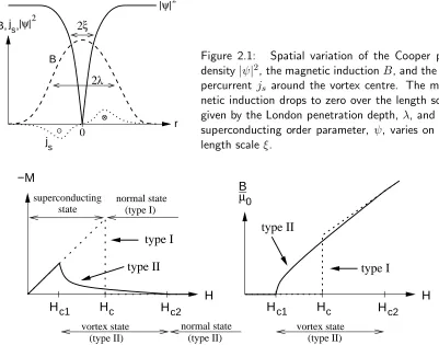
ande the electron charge. Each flux line is surrounded by a supercurrent screening the enclosed magnetic induction. Figure 2.1 on the following page shows the mag-netic induction and the superconducting order parameter in the neighbourhood of a vortex.

Type-I superconductors with κ < 1/√2 expel an external magnetic field com-pletely up to a critical field value Hc at which the superconductivity breaks down, as demonstrated schematically in figure 2.2 on the next page (dotted line). Type-II superconductors show the same behaviour for small fields but only up to field strengths Hc1 < Hc. For field strengths between Hc1 and Hc2, the external field

(21)

j_s j_s

|ψ|2 |ψ|2

0 r

B, ,

B

ξ

λ

[image:21.595.121.522.74.389.2]

2 2

Figure 2.1: Spatial variation of the Cooper pair density_|ψ_|2_{, the magnetic induction}_B_{, and the} su-percurrent js around the vortex centre. The

mag-netic induction drops to zero over the length scale given by the London penetration depth,λ, and the superconducting order parameter, ψ, varies on the length scaleξ.

(type II) (type II) (type I)

(type II)

H_c2 H_c

H_c1 H_c1 H_c H_c2

0 µ

B

H H

−M

type I

vortex state normal state normal state

superconducting state

vortex state

type I type II

type II

Figure 2.2: Different behaviour of magnetisationM (left) and magnetic inductionB (right) to an external applied magnetic field H in I and II superconductors. In type-II superconductors, vortices start penetrating the material at Hc1 and represent B within the sample. At Hc2 the vortex cores overlap and the external field Hc2 is established as superconductivity breaks down.

work. Because of the partial flux penetration, the diamagnetic energy cost of ex-pelling the field is reduced and therefore Hc2 can be significantly larger than Hc. This property has made high-field superconductors possible.

In the mixed state, vortices tend to align in a hexagonal lattice to minimise their energy. This will be discussed in more detail in section 2.4.

The critical fields Hc1 and Hc2 are functions of the temperature and decrease

with increasing temperature. In figure 2.3 we show the phase diagram of a type-II superconductor as a function of magnetic field and temperature. At zero tem-perature, we can estimate Hc1 ≈ _κ1Hc and Hc2 ≈ κHc (Kittel, 1996). For

high-temperature-materials, the Ginzburg-Landau parameter is big (κYBCO ≈ 90 and

κBSCCO ≈60) and therefore Hc1 is much smaller than shown in figure 2.2 and 2.3.

In this work the regime H Hc1 is investigated and hence B ≈µ0H, where µ0

(22)

H

_c2

T

_c

H

_c1

H

T

0

mixed phase

Meissner phase

state normal

Figure 2.3: Phase diagram of type-II super-conductor

2.3

Interactions in the vortex state

2.3.1 Lorentz force and flux flow

In the presence of a transport current, a Lorentz force fL per unit length,

propor-tional to the current density j acts on the vortices and pushes them in a direction perpendicular to the transport current and perpendicular to the orientation of the magnetic field

f_L =j_×Φ₀, (2.1)

whereΦ0is a vector pointing in the direction of the magnetic field with a magnitude

of the magnetic flux quantum Φ0.

For an ideal homogeneous material, Bardeen and Stephen (1965) showed that the resulting motion of vortices with velocity v is resisted by a viscous drag force

fvisc =−ηvolumev per unit volume with a viscosity coefficientηvolume per unit volume

given by

ηvolume =B2/ρff and ρff ≈ρnB/Bc2, (2.2)

with ρff the flux flow resistivity, ρn the normal state resistivity of the material,

B the magnetic induction, and Bc2 the upper critical value of B at which

super-conductivity breaks down. Equation (2.2) has been confirmed in experiments, for example by Kunchur et al. (1993). The normal state resistivity enters the expres-sion because the moving vortices induce local electric fields (due to the magnetic induction changing with time) which act on the unpaired non-superconducting elec-trons. There is another contribution coming from the change of the Cooper pair density on a time scale comparable to the relaxation time of the Cooper pair system (Buckel, 1993, p.181).

(23)

|ψ|2

b) a)

r r

Imperfection Vortex

Figure 2.4: a) Schematic plot of the density of Cooper pairs in the neighbourhood of an imperfection in the crystal structure and a vortex. b) If the vortex is placed into the imperfection then the system’s energy is reduced.

2.3.2 Pinning

In practice, real materials always have inhomogeneities, which tend to “pin” vortices to the atomic crystal structure. Therefore, for currents below a critical current density, the vortices are pinned and do not respond to a small Lorentz force, so no resistance is measured.

Imperfections in the crystal structure influence the motion of vortices via scat-tering or the suppression of the superconducting order parameter (Blatter et al., 1994, p.1143). The latter mechanism can be explained qualitatively in terms of the energy contribution of the condensation energy to the superconducting state and is illustrated in figure 2.4. Imperfections in the periodicity of the atomic structure locally inhibit superconductivity. In these areas, there is no negative contribution from the condensation energy to the total energy of the superconducting state. The net reduction in system energy of a vortex in a type-II superconductor is positive, and the core of the vortex is not superconducting. It is therefore energetically ad-vantageous if a vortex is located in an imperfection. Any attempt to move it from there to another position would increase the system energy. For forces which are not too large the vortex is pinned.

(24)

2.3.3 Vortex-vortex interactions

In addition to the Lorentz force and the pinning interaction a third force acting on vortices is their mutual repulsion.

All high-temperature superconductors known to date, such as YBCO and Bi2Sr2CaCu2O8 (BSCCO), are layered materials, i.e. superconducting CuO2

lay-ers alternate with less superconducting laylay-ers. A vortex line can be undlay-erstood as a coupled line of two-dimensional “pancake” vortices which occupy the CuO2 layers

(Artemenko and Kruglov, 1990,Feigel’man et al., 1990,Buzdin and Feinberg, 1990,

Clem, 1991). The following is a short summary of the different kinds of electromag-netic interaction between pancake vortices in single and stacked two-dimensional layers (Clem, 1991,Blatter et al., 1994, pp.1277,Clem, 1998).

2.3.3.1 Two pancake vortices in an isolated superconducting thin film

The energy U(r) of two pancake vortices separated by a distance r= px2₊_y2 _in

a thin film of thickness d is given by Pearl’s solution (Pearl, 1964)

U(r) = Φ

2 0d

2πµ0λ2s

H0 _r

Λ

−Y0 _r

Λ

(2.3)

whereλs≈1000˚A is the London bulk penetration depth, andΛ= 2λ2s/d≈3·105˚A is the two-dimensional thin film screening length. The quoted numbers are charac-teristic of an YBCO layer and are given to provide a feel for the order of magnitude of the different lengths. H0 and Y0 are the Struve function and the Bessel function

of the second kind.

The bulk penetration depth, λs relates to the in-plane penetration depth of a thin layer, λab ≈ 1400˚A, via λs = λab

p

d/s, where d _≈ 6˚A is the layer thickness and s_≈12˚A is the layer spacing. We re-write Λ= 2λ2

ab/s, and introduce

0 =

Φ2 0

4πµ0λ2ab

, (2.4)

with µ0 = 4π·10−7 Vs_Am being the vacuum permeability and Φ0 the magnetic flux

quantum. Eventually, we can express the interaction (2.3) strength in terms of0

U(r) = 20s

H0 _r

Λ

−Y0 _r

Λ

(25)

For small and larger, the following approximations hold:

U(r)_{∝ −}ln _Λr : rΛ (2.6)

U(r)_∝ 1

r : rΛ. (2.7)

2.3.3.2 Two pancake vortices in one layer in a system of stacked thin films

Due to induced screening currents in the layers above and below the “central” layer (which holds one pancake vortex), the resulting current distributions are different from those in the isolated thin film. For the repulsive force between two vortices in one layer in an infinite system of stacked layers it has been shown (Clem, 1991, eqn. 27) that the interaction forceF(r) is given by

F(r) = 20s

1

r

1₋ λab

Λ

1₋exp

− r

λab

. (2.8)

Since λab/Λ≈10−3, this is effectively

Fr(r) = 20s

r . (2.9)

This corresponds to a potential

U(r) =₋20sln (r) (2.10)

which is logarithmic at all distances, not just forrΛ as in the isolated thin film (2.6).

For the electromagnetic interaction of two pancake vortices in different layers an attractive force is found that is weaker than the in-layer repulsion by a factor of approximatelyλab/Λ. We consider this in detail for the studies of three-dimensional

pancake systems in chapter 6.

2.3.3.3 Two stacks of aligned pancake vortices

For aligned stacks of pancake vortices where the magnetic field is perpendicular to the superconducting planes as shown in figure 2.5 on the following page, the interaction energy per unit length between two such stacks is found to be

U(r) = 20K0

r λab

. (2.11)

K0 is the modified Bessel function of the second kind. Equation (2.11) shows the

(26)

B

x y

s

z

Figure 2.5: A stack of aligned two-dimensional vortex pancakes.

energy of two vortex lines in a continuous medium (Tinkham, 1996, p. 154). In the latter result λab is given by λs, the isotropic London penetration depth. K0(r/λab)

can be approximated with

K0

r λab

=

  

q

πλ

2r exp

− r λab

: r _{→ ∞}

ln λab

r

+ 0.12 : r λ. (2.12)

In contrast to equation (2.10) the interaction energy drops off exponentially for large distances. This is due to the weak attraction of pancakes in different layers.

In the remainder of this work, we are dealing with λab rather than λs. We therefore use λ_≡λab to shorten our notation.

(27)

H

_c1

T

_c

H

0

lattice

T

Meissner phase

liquid

liquid vortex

vortex

normal state

Figure 2.6: The vortex state in the absence of pinning but considering thermal fluctua-tions. The plot is based on figure 2 from Blatter et al. (1994). Large parts of the diagram are occupied by the molten vortex lattice.

2.3.4 Summary

The vortex state is determined by the relative strengths of the following energies:

• the vortex-vortex interaction which favours a hexagonal lattice,

• the vortex-pinning energy which (generally) introduces disorder and

• the thermal energy which destabilises the lattice further.

The Lorentz force drives the system over the pinning energy surface and this results in complex vortex dynamics.

2.4

Static vortex phases

2.4.1 The vortex phases without pinning

We have shown the conventional picture of a clean superconductor (i.e. without pinning) in figure 2.3 on page 8: in the Meissner phase the material shows perfect diamagnetism, and between the two critical fields Hc1 and Hc2 vortices penetrate

the sample and arrange in a hexagonal lattice. On crossing the upper critical field

Hc2 the vortex cores overlap, and the material becomes normal.

If one considers the hexagonally arranged vortices as “vortex matter” than it would be plausible to assume that the vortex crystal could melt at a sufficiently high temperature. This is indeed the case although in conventional superconductors the melting transition line lies so close to the upper critical field line that they are virtually indistinguishable (Br´ezin et al., 1985). It was first predicted by Nelson

(28)

We add thermal fluctuations to the phase diagram and show the result in figure 2.6, which is based on figure 2 from Blatter et al.(1994). The vortex lattice phase can melt either due to an increase in temperature (in which case thermal fluctuations destroy long-range order), or the vortex lattice can melt due to a decrease of the field. In this case the vortex separation becomes large and the interaction between vortices becomes exponentially weak. This results in a decaying shear-modulus which softens the lattice until it melts. Note that the figure is not drawn to scale in order to emphasise the main structures appearing in the diagram, and that the dilute vortex liquid exists only for a very small range of H. We will not consider the Meissner phase and the re-entrant liquid phase at very low fields H _≈ Hc1 in

the remainder of this work.

The position of the melting line can be estimated with a Lindemann1 _criterion

(Blatter et al., 1994, 1996, Vinokur et al., 1998), but the nature of the transition cannot easily be determined. The challenge in defining a theoretical scheme de-scribing vortex-lattice melting follows from the complexity of the vortex system in real (three-dimensional) superconductors combined with the general lack of exact theories of melting (Dodgson et al., 2000b). We address this issue in chapter 6 and study the melting transition for a layered system of pancakes that interact electro-magnetically with each other.

2.4.2 The static phases in presence of pinning

The theoretical treatment of a system of vortices under the influence of pinning objects is difficult as it is a many-body problem with competing interactions. Due to the vortex-vortex interaction, the vortices repel each other and try to establish the hexagonal Abrikosov lattice as introduced in section 2.2. At the same time, the underlying pinning potential deforms the vortex lattice such that as many vortices as possible have a low pinning energy. However, this happens at the expense of increasing the vortex lattice elastic energy by deforming it. The equilibrium vortex configuration is the one which minimises the sum of the lattice deformation and the pinning energy.

For random point pinning,Larkin and Ovchinnikov (1979) presented their elastic theory of collective pinning which describes the distortion of the flux line lattice in terms of correlation volumes Vc = R2cLc in which the vortex lattice is reasonably

1_{The empirical Lindemann criterion (}_Lindemann_{, 1910) assumes that a crystalline lattice}

be-comes unstable with respect to thermal fluctuations of its constitutive elements (atoms, vortex lines, etc.) as the mean-squared amplitude of fluctuations<u2_>_{increases beyond a certain}

(29)

∆

(no dislocations) (dislocations)

Bragg glass 1st order

continuous

disorder strength

temperature T vortex glass or

pinned liquid

[image:29.595.115.285.67.214.2]

liquid

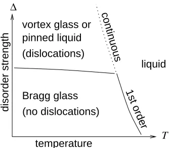
Figure 2.7: Static phase diagram suggested byLe Doussal and Giamarchi (1998) for the elastic man-ifolds in a random potential. The axes show tem-perature T and the strength ∆ of the disordering random potential. This can qualitatively be com-pared with figure 2.6 on page 13 as the disorder strength ∆ relatively increases with the magnetic field (Vinokur et al., 1998).

undistorted. The correlation volume has a length Lc in the field direction and a transverse size of Rc. Rc and Lc are chosen to optimise the trade-off between pinning and elastic energies. One of the main conclusions is that for less than four dimensions any small amount of pinning destroys long-range order.

However, several experimental results were difficult to interpret in this frame-work. For example Bitter decoration experiments for low fields showed remarkably large regions free of dislocations (Grier et al., 1991). Following work byNattermann

(1990),Giamarchi and Le Doussal suggested in 1994 that the Larkin-Ovchinnikov argument may be too simple. They studied the related problem of an elastic pe-riodic medium submitted to a random potential (corresponding to uncorrelated pinning), and found that a “Bragg glass” phase could exist for low fields and weak disordering potentials.

2.4.2.1 Three dimensions

Giamarchi and Le Doussal (1994, 1995) used variational and renormalisation group techniques to investigate the statics of periodic elastic manifolds in random poten-tials, such as vortex lines in superconductors. Following the terminology in the literature, the strength of the random pinning potential is, in short, referred to as “disorder”. They obtain the following three distinct phases for line vortices in three dimensions, which are schematically shown in figure 2.7. A dislocation-free phase with algebraically decaying translational order (i.e. quasi-long-range order) is predicted to exist for sufficiently weak disorder2 _{and temperature. In more detail,}

the translational order correlation function decays like a power law with distance, whereas for short-range order it decays exponentially and for a solid it becomes con-stant for large distances. Although there is no true long-range translational order

2_{For large ranges of parameter space it can be shown that the relative strength of the disorder}

(30)

(as for a perfect lattice withδ-Bragg peaks in the structure factor), the quasi-long-range order still allows low order algebraically diverging Bragg peaks to be observed in the structure factor of such a system, and therefore Giamarchi and Le Doussal called this thermodynamic phase the “Bragg glass” phase. In contrast to a glass in which no periodic lattice structure is visible, a Bragg glass appears as a deformed hexagonal lattice, in which all lattice sites have six nearest neighbours. Thus, from a topological point of view, the Bragg glass is much closer to a solid than a glass, in which translational order decays exponentially, and topological order is destroyed. However, it has many meta-stable states and only quasi-long-range translational order.

For higher fields, Giamarchi and Le Doussal predict an order-disorder transition to a “pinned vortex liquid” or a “vortex glass” which contains topological defects, and for temperatures above the melting temperature, a “vortex liquid”.

The phase transition from the Bragg glass to the liquid is predicted to be first order, whereas the transition from the vortex glass to a liquid is predicted to be continuous (or second order) (Giamarchi and Le Doussal, 1995).

The results as summarised in figure 2.7 seem to be supported by several ana-lytical and numerical studies and compare well with the most recent experiments (for example Kokkaliaris et al., 1999, Klein et al., 2001, and references [47-52] in

Le Doussal and Giamarchi, 1998).

Vinokur et al. (1998) obtained a similar phase diagram using an extended Lin-demann criterion, where the Bragg glass is referred to as a “quasi-lattice” and the vortex glass is referred to as an “entangled solid”. The same orders for the phase transitions are suggested.

2.4.2.2 Two dimensions

The general theoretical belief based on qualitative arguments and simulations (Shi and Berlinsky, 1991, Blatter et al., 1994, Sec.VIII.D.3) is that no solid phase with long-range order exists in two dimensions at finite temperatures in the presence of disorder. However, signatures of melting were observed in experiments in two-dimensional regimes (Yazdani et al., 1994, Theunissen et al., 1996) although on large length scales there was no order (Yazdani et al., 1993). This can be explained by the results of recent theoretical investigations by Carpentier and Le Doussal

(1998) andLe Doussal and Giamarchi (2000) who found that below a length scale

(31)

melting temperature

elastic flow

liquid

force

0

temperature plastic flow

no flow

[image:31.595.115.301.68.195.2]

moving

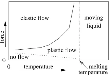
Figure 2.8: Schematic representation of the re-sults ofKoshelev and Vinokur (1994) on the dy-namic phase diagram for a system with a fixed magnetic field and varying Lorentz force and temperature.

topological defects (Giamarchi and Le Doussal, 1998, Sec.3.5) and there may be a two-dimensional Bragg glass phase for all length scales.

In summary, there is some evidence that the two-dimensional Bragg glass phase exists only up to certain length scales, ξD, and not for infinitely large systems, but the existence of the two-dimensional Bragg glass phase is a subtle issue which cannot be answered definitely today. However, in either case the two-dimensional situation is of physical interest, sinceξD can be large and, apart from thin-film superconduc-tors, other two-dimensional physical systems exist such as Wigner crystals (Andrei et al., 1988) and magnetic bubble arrays (Seshadri and Westervelt, 1992) which very likely can be described in the same theoretical framework.

2.5

Dynamic vortex phases

Due to the competing interactions (see section 2.3) in the vortex state, vortices display not only a rich static phase diagram. Also, when being driven by a Lorentz force in the presence of pinning, a wide range of dynamical behaviour can be ob-served, including avalanches, stick-slip dynamics, thresholds for motion, nonlinear and hysteretic response, and plastic and elastic motion.

(32)

Bragg

driving force

∆

disorder strength

F c

F

vortex glass

plastic flow

moving transverse glass

moving Bragg glass glass

[image:32.595.243.426.68.203.2]

?

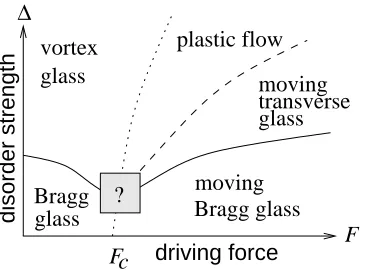
Figure 2.9: Schematic representation of the phase diagram for three-dimensional systems suggested byLe Doussal and Giamarchi (1998) as a function of disorder strength∆and driving force F (at zero temperature). For weak disorder and a weak driving force, a pinned Bragg glass phase with quasi-long-range translational order is expected. For larger driving forces, this depins and becomes a moving Bragg glass. With increasing disorder at low driving forces, the system transforms into a pinned vortex glass (with topological defects and short-range order only). Increasing the driving force from the vortex glass regime results in first plastic flow, then motion in decoupled channels (the moving transverse glass) and for the largest driving forces, a moving Bragg glass is recovered, in which the separate channels couple. Fc

denotes the depinning force. There are no predictions for the behaviour within the regime of the grey box.

more easily and the plastic flow regime extends to larger forces. If the temperature is higher than the melting temperature, the system behaves as a liquid.

For larger driving forces Koshelev and Vinokur observed a dynamical ordering of the system which is in agreement with other simulation results (Shi and Berlinsky, 1991, Olson et al., 1998b). They also predicted the existence of a dynamic phase transition at some characteristic “crystallisation” current. The underlying argument was that for a strongly driven system the pinning potential is felt as a random force and that this can be expressed as an effective “shaking temperature” which is inversely related to the velocity of the system. For large enough driving forces the system is predicted to crystallise into a perfect lattice.

Recently Giamarchi and Le Doussal (1996) extended their description of the statics of the vortex state to the dynamics, predicting a “moving” Bragg glass. Shortly afterwards, Balents et al. (1997) commented on Giamarchi and Le Dous-sal’s publication, predicting that, in addition to the moving Bragg glass, a moving “smectic” should exist. They later detailed this (Balents et al., 1998), and their ideas contributed to the detailed work of Le Doussal and Giamarchi (1998).

2.5.1 Three dimensions

Figure 2.9 shows a schematic sketch of the dynamic phase diagram suggested by

(33)

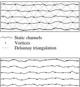
Vortices Static channels

Delaunay triangulation

[image:33.595.114.271.81.250.2]

Figure 2.10: The moving Bragg glass. A driving force is acting horizontally from left to right. Vortices move along static channels like beads on a string. Vortices in different channels are coupled and move with the same average velocity in the horizontal direction. There are no dislocations in the system.

Figure 2.11: The moving transverse glass. Vortices move in static channels, but vortices in different chan-nels can move with different velocities. The chanchan-nels are decoupled, and dislocations between different chan-nels exist.

forceF (at zero temperature). For low disorder and weak driving forces the system is expected to be pinned and to form a Bragg glass as described in the static case (section 2.4.2.1). For stronger disorder it is expected to be pinned as a disordered vortex glass, as in the static case. Increasing the driving force in this regime leads to a plastic flow phase where vortices move more or less independently of their neighbours. For further increases of the driving force, a moving transverse glass phase and moving Bragg glass phase are predicted to exist.

2.5.1.1 The moving Bragg glass

(34)

static channels move with the same average velocity in the direction of the driving force, and the system retains topological order.

2.5.1.2 The moving transverse glass

In contrast, for smaller driving forces or stronger disorder the “moving transverse glass” is expected, as sketched in figure 2.11 and first predicted by Balents et al.

(1997). Vortices move along static channels, but the motion between different channels is not necessarily coupled. The average horizontal velocity can vary from static channel to static channel such that phase-slips may occur, and thus there can be topological defects between two channels moving with different velocities. It is expected in the moving transverse glass that channels are coupled up to a certain length (perpendicular to the channel orientation), and that phase slips occur between chunks of such coupled channels. The length scale of coupled channels increases with the driving force and decreases with the disorder strengths. In the limit of small pinning or large driving forces, consequently, all channels are coupled, and the moving Bragg glass is recovered.

In terms of “dynamic Larkin domains” (over which the vortices form a relatively undisturbed lattice) in the drifting vortex system, the moving transverse glass is due to a strong anisotropy in the Larkin lengths,Rkc-parallel to the driving direction and

R⊥

c-perpendicular to the direction of the driving force (Le Doussal and Giamarchi,

1998, Scheidl and Vinokur, 1998).

Different names for the Moving Bragg Glass (MBG) and the Moving Transverse Glass (MTG) are in common use: in the work ofBalents et al. (1998) the moving Bragg glass is termed “moving lattice”, and the moving transverse glass is called a “moving smectic”. Scheidl and Vinokur (1998) came to similar conclusions for the dynamic phase diagram asBalents et al.(1998) andLe Doussal and Giamarchi

(1998) using a perturbative approach, and call the moving Bragg glass “coherent phase” and the moving transverse glass “decoupled channels”.

2.5.2 Two dimensions

(35)

c F

disorder strength

driving force F

∆

plastic flow

vortex

glass moving

[image:35.595.118.523.80.474.2]

transverse glass

Figure 2.12: Schematic representation of the phase diagram for two-dimensional systems suggested byLe Doussal and Giamarchi (1998) as a function of disorder strength ∆ and driv-ing force F (at zero temperature). It has been assumed that there is no topologically ordered static phase for finite disorder strength and zero driving force. Whether there is a moving Bragg glass phase at large driving forces (in which the decoupled channels of the moving transverse glass couple) is currently not known. No such phase is shown in this figure.

0 5 10 15

0 1 2 3 4 5 6 7

pinning strength (f

0

)

driving force (f₀)

coherently moving structure decoupled channels plastic flow

vortex glass

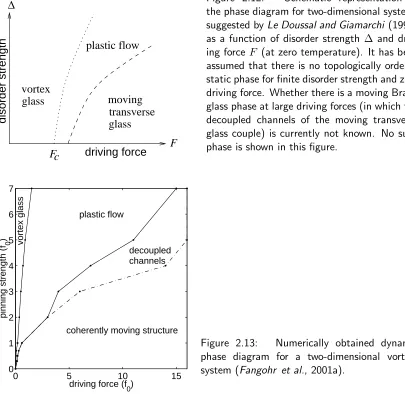
Figure 2.13: Numerically obtained dynamic phase diagram for a two-dimensional vortex-system (Fangohr et al., 2001a).

ordered state for any finite disorder strength. Above the depinning driving force,

Fc, highly filamentary plastic flow is expected at first, which transforms into a moving transverse glass for even higher driving forces. Whether the decoupled static channels that constitute the moving transverse glass couple for large velocities cannot be decided at present. In the figure no such moving Bragg glass phase is shown.

Recent two-dimensional Langevin dynamics simulations (Olson et al., 1998b,

(36)

v_t

F_t

linear

T=0 T>0

transverse driving force

transverse velocity

[image:36.595.117.299.70.243.2]

Ftc

Figure 2.14: Schematic representation of the transverse current-voltage relation predicted by Le Doussal and Giamarchi (1998) for the mov-ing glass. Shown is the velocity vt transverse

to the main direction of motion as a function of a transverse driving force Ft. At zero

tempera-ture the system does not respond to transverse driving forcesFt < Ftcbelow a critical transverse

forceF_tc. For finite temperature a linear response in velocity is expected for finite and small trans-verse driving forces, as shown by the dotted line. For Ft nearFtc the finite temperature curve

ap-proaches the zero-temperature curve.

structure could be a moving Bragg glass, or it could be the decoupled channel regime in which the channels are so broad that they cover the complete simulation cell. Thus, it cannot be decided whether the numerical data from a two-dimensional simulation correspond more closely to the three-dimensional prediction (figure 2.9) or the two-dimensional prediction (figure 2.12 on the preceding page). However, the existence of the moving glass phase is confirmed.

2.6

The critical transverse force

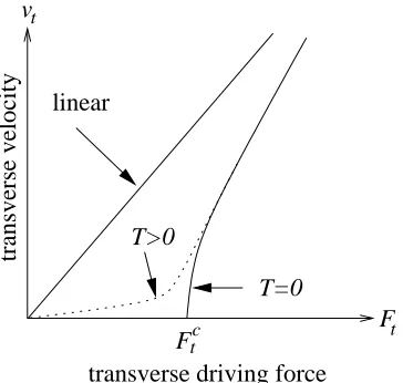
Giamarchi and Le Doussal (1996) found that for the moving glass there should be a finite transverse barrier for a system moving along one of its principal axes at zero temperature. To investigate this, one drives a system in the moving glass regime, where it is moving along a principal lattice axis. Once a steady state has been found and the rough time-independent channels have developed, one applies a small driving force transverse to the direction of motion. Experimentally, this can be achieved by applying a small second current transverse to the first current which drives the system. It is predicted that for small enough transverse driving forces the system does not leave the static channels. Only for transverse forces exceeding a critical force, does the system start to move transversely. The expected trans-verse current–transtrans-verse voltage (or equivalently transtrans-verse driving force–transtrans-verse velocity) relation is shown figure 2.14.

(37)

near to the zero temperature critical transverse force, the curve approaches the zero-temperature curve.

The transverse critical force is a rather subtle effect, even more so than the usual longitudinal critical force. It does not exist for a single particle in a random potential, although a single particle does experience a non-zero longitudinal critical force. The transverse critical force is a dynamical effect due to barriers preventing the channels re-orienting. The transverse critical force has been proposed to be the order parameter of the moving glass phase at zero temperature (Le Doussal and Giamarchi, 1998). If there is a transverse critical force in a moving state, then there should be a history dependence in the system.

In numerical work, a critical transverse driving force has been found in two dimensions (Ryu et al., 1996, Moon et al., 1996,Olson and Reichhardt, 2000), but to the best of our knowledge, no such experimental results have been published yet. We address the critical transverse force in chapter 5.

2.7

Summary

The theoretical models introduced here (Giamarchi and Le Doussal, 1996,Balents et al., 1998, Le Doussal and Giamarchi, 1998, Scheidl and Vinokur, 1998) are the best description of the statics and dynamics of the vortex state currently available and increasingly experimental data are interpreted within these frameworks. How-ever, there are many open questions within these models which cannot be answered analytically, but have to be investigated experimentally and numerically.

2.8

Applications

Apart from a strong interest in basic research in the (non-equilibrium) statistical mechanics of (driven) systems with quenched disorder, there is a wide range of practical applications of high-temperature superconductivity which are currently used or could be very useful in the future.

Macroscopic superconducting devices are nowadays mainly used to provide strong magnetic fields for various applications such as medical magnetic resonance imag-ing (MRI) machines, and for particle accelerators. There are applications such as non-exploding fault current limiters and superconducting voltage transformers in the electric power industry.

(38)

are determined by the behaviour of vortex lines, and that is the physical system under investigation in this thesis.

On a much smaller scale superconducting filters have very highQ-values and im-prove bandwidths and selectivity of telecommunication receivers. Finally, supercon-ducting quantum interference devices (SQUIDs) are used to detect magnetic fields of strengths of a few femto-tesla. This allows magneto encephalography (MEG) mea-surements of the magnetic fields generated by electric currents in human brains. Another application of these highly sensitive sensors is non-destructive evaluation (NDE) of aeroplane wings, wheels and rivets.

(39)

Chapter 3

The Simulation

This chapter describes the computer simulation that has been developed and used for this work. The central idea is to represent vortices as massless classical particles that are free to move in a two-dimensional area. Those particles can be identi-fied with vortex-lines when modelling thin films in which vortices are “stiff”. To model three-dimensional systems we associate these particles with pancake-vortices, and use a mean field approach (chapter 6) to account for interactions in the third dimension.

In section 3.1, an overview of techniques to simulate many-body problems is given and in section 3.2 these techniques are related to the vortex state, followed by a detailed description of the simulation software. This includes the derivation of the central equations of motion in section 3.3 and methods to solve them (section 3.4). In sections 3.5 we describe the boundary conditions and section 3.6 details our choice of simulation units. Section 3.7 assesses the applicability of the model, and in section 3.8 the observables to monitor the simulation are introduced. Section 3.9 concentrates on practical aspects of the usage of the simulation software such as the user interface, and hardware and software requirements. A summary is provided in section 3.10.

3.1

Computer simulations of many-body systems

Computer simulations have proved to be a valuable tool for problems that cannot be solved analytically. Numerical solutions are particularly useful for providing results for specific parameters which are not at all obtainable otherwise.

(40)

Stochastic

Deterministic

Hybrid Methods Langevin Dynamics

Molecular Dynamics

Force Biased Monte−Carlo

Metropolis Monte−Carlo Figure 3.1: Monte Carlo simulations work stochastically and molecular dynamics sim-ulations work deterministically. There are various techniques that combine both meth-ods.

Monte Carlo simulations are adopted from general Monte Carlo methods for solving high-dimensional integrals. In Monte Carlo simulations the integrals of interest are the statistical mechanics ensemble averages for a property f(rN_{), for} example in the canonical ensemble:

< f >= R

. . .R dr1dr2. . .drN f rN

exp₋U_k(rN)

BT

R

. . .R dr1dr2. . .drN exp

−Uk(BrNT)

. (3.1)

This is the standard case where the number of particles N, the temperatureT, and the volume V of the simulation are given. The vector rN has N d components when each particle’s position ri has d components, and U(rN) is the energy of the system. Since Monte Carlo methods are generally not well suited to study dynamical quantities, the integration in phase space over the generalised momenta p1, . . . ,pN has been carried out already in equation (3.1).

Taking the Boltzmann factor exp₋U_k(rN)

BT

into account, it was suggested by

Metropolis et al.(1953) to consider only configurations which contribute most to the integral. This is known as importance sampling for general Monte Carlo methods and in the context of Monte Carlo simulations it is referred to as the “Metropolis algorithm”.

(41)

Molecular dynamics methods can be divided into equilibrium and non-equilibrium dynamics. Equilibrium dynamics are usually applied in the micro-canonical ensem-ble to an isolated system with energy E, containing a fixed number of particles

N, in a fixed volume V. However, there exist methods to fix the simulated tem-perature, which allows investigation of canonical ensembles (for exampleRapaport, 1995). In non-equilibrium molecular dynamics, an external force is applied to the system to establish non-equilibrium situations of interest. The particles’ positions are obtained by integrating Newton’s equation of motion. For a set ofN particles with positions ri, the set of equations to solve reads1

mi¨ri =Fi(r1,...,N,r˙1,...,N, t) i = 1, . . . ,N, (3.2) wheremi is the mass of particlei, andFi is the total force acting oni. The velocity of particle i is ˙ri and ¨ri is its acceleration.

To compute a system property f(rN_,_r_˙N_{), one takes the time average of that} property

< f >= lim t→∞

1

t

t0+t Z

t0

dt0 _f _rN₍_t0₎_,_r_˙N₍_t0₎_. _(3.3)

In contrast to the Monte Carlo simulations, it is here easily possible to investigate dynamical quantities such as transport coefficients and time correlation functions. According to the ergodicity hypothesis the ensemble average in equation (3.1) and the time average in equation (3.3) should be the same.

Force biased Monte Carlo methods compute the force exerted from all other par-ticles on particlei and then move that particle iin this direction. This reduces the number of trial moves required, but each sweep is computationally more expensive.

Hybrid methods are Monte Carlo simulations that use a sequence of molecular dynamics steps to generate new random configurations. This ensures that very different areas in phase space are covered and reduces the number of Monte Carlo sweeps required to study equilibrium properties of the system.

Langevin dynamics were developed to investigate Brownian Motion (Lenk and Gellert, 1989, p.537). One studies particles immersed in a continuum, for example a fluid. Instead of considering all microscopic interactions of all particles establishing the fluid, one concentrates on one particle and its interactions with the continuum. The force exerted on the particle by the fluid is broken into two parts: an average

1_{The following convention is used: the dot notation represents the time derivative: ˙}_r₌ dr

dt and

¨ r= d2

r

(42)

viscous force₋η˙r_i and a random force χ(t) whose time average is zero (Kubo et al., 1985, p.14). The equation of motion for particle iis

mi¨ri =−η˙ri+χi+F0i, (3.4) whereF0_i represents all forces not covered in the other two terms. The macroscopic frictional force represents an averaged value of many microscopic interactions. In cases where inertial effects are small, the massmi of the particles can be set to zero. That reduces the system of differential equations of second order in (3.4) to a system of first order equations which are occasionally referred to as the “overdamped” Langevin equations of motion because the absence of the inertial term causes the motion to be overdamped.

3.2

Methods to simulate the vortex state

The most direct method to investigate the vortex state is to solve the (time-dependent) Ginzburg-Landau differential equations numerically to obtain solutions for the complex valued order parameter ψ and the magnetic vector potential. The set of coupled non-linear partial differential equations can be solved on a discrete grid, as demonstrated for example by Braun et al. (1996),Gropp et al. (1996) and

Aranson and Vinokur (1998). On the one hand this approach does not simplify the physical situation, but on the other hand it is computationally very demanding since it requires many grid points to resolve even a single vortex.

Another starting point is to treat vortices as structureless point- or string-like objects. Each of the areas in which the superconducting order parameter ψ drops to zero is mapped to such an object, which is then considered as being a classical particle. To compute the interactions between these classical particles one uses effective interaction potentials (for example Clem, 1991, Bulaevskii et al., 1992). The price which has to be paid for decreasing the computational complexity is that the small length scale ξis lost and phenomena like pinning, vortex-anti-vortex creation or flux cutting do not come intrinsically with these models, but have to be implemented by other means. To study the statics of the vortex state, Monte Carlo simulations can be used (for example T¨auber and Nelson, 1995,Yates et al., 1995, Ryu and Stroud, 1996), whereas to study the dynamics, Langevin dynamics methods are required (for example Brass et al., 1989, Koshelev and Vinokur, 1994,

(43)

van Otterlo et al., 1998,Kohandel and Kardar, 1999). Here, we follow this approach and use Langevin dynamics to study the static and dynamic behaviour of vortices. Parts of this work are applicable to particle simulations in general and not limited to vortex state simulations. Therefore, we frequently use the term “particle” instead of “vortex”.

In addition to the methods described above, there are other approaches to simu-late the physics of the vortex state. These range from xy-models (for exampleLi and Teitel, 1994, Nguyen and Sudbø, 1999) to the solving of a coarse grained equation of motion for the displacement field (Aranson et al., 1998), investigating a disor-dered array of Josephson junctions (for exampleDom´ınguez, 1999), mapping vortex lines to bosons (for exampleNordborg and Blatter, 1997) and combination of meth-ods, such as the London-Langevin method coupled to solving the time-dependent Ginzburg-Landau equation (Bou-Diab et al., 2001).

3.3

Equation of motion

The terms in the equation of motion that influence the behaviour of each vortex are the viscous force and a stochastic term from the Langevin equation (3.4), the vortex-vortex interaction, the Lorentz force, and pinning forces. Each of these will be presented in detail in the following subsections.

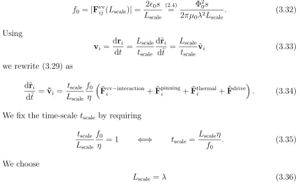
3.3.1 Overdamped Langevin dynamics

The Langevin dynamics as introduced in section 3.1 form the physical basis of this simulation. The flux motion is strongly overdamped since the viscous force is much greater than any possible inertial forces (Brandt, 1995, Sec. 5.2) and the vortex mass can be ignored. The mass termmion the left-hand side of equation (3.4) is set to zero and the remaining Langevin equation for vortexireads (withχi =Fthermali ): 0 =₋η˙r_i(t) +F_ivv−interaction(r1(t), . . . ,rN(t)) +Fdrive(t) +Fthermali (t) +Fpinning(ri(t)). (3.5) The terms represent from left to right: the viscosity term, the forces from the vortex-vortex interaction, the drive or Lorentz force acting on all vortices equally, the noise term which introduces temperature, and the pinning force which depends on the position of the vortex.

3.3.2 Viscosity

(44)

viscous drag coefficient per volume is

ηvolume ≈

BBc2

ρn

. (3.6)

Considering that the magnetic induction, B, is represented by N vortices, each carrying a flux quantum Φ0 over the area A, leads toB =NΦ0/A. Equation (3.6)

can be converted into the viscosity per vortex per unit length η1

length = ηvolumeN A ≈

Φ0Bc2

ρn .The viscosityηin equation (3.5) is given by the viscosity per (pancake) vortex which for a (pancake) vortex of length s is

η=η_length1 s= Φ0Bc2

ρn

s. (3.7)

3.3.3 Vortex-vortex interaction

The energyU and force F per unit length of interacting stiff vortex lines separated by a distance r is (see section 2.3.3)

Uline(r) = 20K0 _r

λ

⇐⇒ Fline(r) =

20

λ K1

_r

λ

(3.8)

and the interaction energy and force between pancakes in the same layer is effectively (see section 6.2 for details)

Upancake(r) = 20sln

λ r

⇐⇒ Fpancake(r) =

2s0

λ

1

r (3.9)

where0 = Φ 2 0

4πµ0λ2,λis the London penetration depth, andsis the layer separation. For simulations of isolated thin-films, the vortex-vortex interaction is given by Pearl’s solution (2.3).

We have implemented all three relevant interactions ( ln, K0 and Pearl’s

solu-tion), and the interaction potential can be chosen in the configuration file (section 3.9.2.1). We use the smooth cut-off as described in chapter 4 to overcome problems resulting from truncating the interaction.

Using, for example the logarithmic interaction potential (3.9), the vortex-vortex interaction force Fvv_ij felt by pancake i from pancake j at positions ri and rj, re-spectively, reads

Fvv_ij(r_i₋r_j) = 20s

1

|ri−rj|

ri−rj

|ri−rj|

=