Biological Oceanography by Remote Sensing
M.A. Srokosz
in
Encyclopedia of Analytical Chemistry
R.A. Meyers (Ed.)
pp. 8506–8533
Biological Oceanography by
Remote Sensing
M.A. Srokosz
Southampton Oceanography Centre,
Southampton, UK
1 Introduction 1
1.1 A Brief History of Ocean Color
Measurements from Space 2
2 Light in the Ocean 3
2.1 Some Definitions 3
2.2 In-water Constituents and Bio-optics 4
2.3 Measurements from Space and the
Effect of the Atmosphere 5
2.4 Case 1 and Case 2 Waters 6
3 Satellites and Sensors 6
3.1 Missions and Sensors Characteristics 6
3.2 Algorithms, Including Atmospheric
Correction 9
3.3 Calibration and Validation 10
4 Applications 11
4.1 Measurements of Phytoplankton 11
4.2 The CO2 Problem 15
4.3 Biophysical Interactions 17
4.4 Assimilation of Data into Models 20
4.5 Dimethyl Sulfide, Climate, and Gaia 22
4.6 Commercial Application – Fisheries 22
4.7 Possible Future Applications 22
4.8 Afterword 23
Acknowledgments 23
Abbreviations and Acronyms 23
Related Articles 24
References 24
Biological oceanography may be studied from space using sensors on satellites that determine the color of the ocean. The presence of phytoplankton (microscopic algae) in the upper layers of the ocean changes the color of the water as seen from above. In simplified terms, this is due to the selective absorption of blue light by the phytoplankton pigments (primarily chlorophyll) which changes the appearance of the water from blue to green. These changes in color can be observed using a satellite-borne spectroradiometer that measures the water-leaving radiance in a number of bands in the visible part of the electromagnetic spectrum. The limitations of the technique
are first, that only information on the phytoplankton in the upper layers of the ocean can be obtained (light does not penetrate very far into the ocean). Second, most of the signal measured by the satellite sensor originates in the atmosphere (due to the molecular and aerosol scattering of photons there), so careful correction for atmospheric effects is necessary if good ocean data are to be obtained. Of course, in the presence of clouds the sensor will not ‘‘see’’ the ocean surface at all, and no data will be obtained. Third, only one component of the ocean ecosystem, namely the phytoplankton, can be studied by this means. Despite these limitations, satellite observations of ocean color have given new insights into biological oceanography on a global scale that could not have been obtained by any other means of observation. Observations of ocean color have contributed to a better understanding of the biophysical interactions that determine the phytoplankton productivity, the seasonal and interannual variations of the phytoplankton biomass on global scales, and the role of phytoplankton in the climate system. They have also contributed to the improved modeling of biogeochemical processes in the ocean.
1 INTRODUCTION
The purpose of this article is to describe the application of satellite remote sensing techniques to the study of biological oceanography. In one sense it seems strange to think that a sensor (instrument) flying on a satellite several hundreds of kilometers above the ocean surface can tell us anything at all about the biology of the ocean. This initial reaction is to a large extent correct, in that measurements from space can only tell us something directly about one very specific component of the ocean biology. That component is the phytoplankton, microscopic plants that live in the near-surface waters of the ocean. The reason that this component can be observed from space is that the phytoplankton contain pigments that are necessary for photosynthesis (primarily chlorophyll-a) and their presence in the water changes the color of the water, as seen from above the sea surface, usually from blue to green. Thus a satellite-borne sensor that makes measurements in the visible part of the electromagnetic spectrum can be used to measure the change in color, and so provide information on the phytoplankton.
Given that only a single component of the ocean biological system can be measured from space, one might ask: why bother? Plankton are the most abundant life form in the world’s oceans, both in terms of weight and of numbers. Phytoplankton are microscopic plants, while zooplankton are the microscopic and small animals that feed on the phytoplankton. A cubic meter of seawater
Encyclopedia of Analytical Chemistry
will contain millions of these small plants. Phytoplankton are the oceanic equivalent of terrestrial plants, forming the basic element of the oceanic food chain. The total phytoplankton biomass is greater than that of all the marine animals taken together (zooplankton, fish, and so on). In addition to their role in the food chain, they have a significant role in the world’s climate system. Their presence in the water causes light to be scattered and absorbed, which warms the upper layers of the ocean. They produce chemical compounds that escape into the atmosphere and have a role in the formation of clouds. More fundamentally, in growing they use carbon dioxide from the atmosphere that has been absorbed into the ocean. When they die, some proportion of the plankton fall out of the upper layers of the ocean and become part of the seabed sediments, thus removing carbon from the system. Therefore, phytoplankton have a major role in the global carbon cycle and may be important in either ameliorating or accelerating the effects of anthropogenic emissions of CO2into the atmosphere. At the present time it is not known how the phytoplankton will respond to the warming occurring due to the increase of greenhouses gases..1/
The preceding paragraph shows the importance of phytoplankton and why measuring them and their behavior is necessary, but why do it from space? As noted above, phytoplankton are ubiquitous in the world’s oceans, but the traditional ship-based methods of observation are unable to give a truly global view of the phytoplankton in the ocean. Thus observations from space are the only means of obtaining a global view. In order to understand the oceanic ecosystem, of which phytoplankton are just one component, ship-based and other types of measurements are still necessary. However, the ability to measure one component of the system from space has brought many new insights into the biology of the ocean on the global scale. These will be described later in this article.
There are, of course, drawbacks to measuring phyto-plankton by satellite remote sensing methods. Since the measurement of ocean color is made using the visible part of the electromagnetic spectrum, the major problem that arises is the presence of clouds, which prevents the sensor from seeing the sea surface and thus making measure-ments. (Other satellite sensors that measure in a different part of the electromagnetic spectrum, particularly the microwave part, can see through clouds, but do not pro-vide information on ocean biology directly)..2 – 4/As some areas of the world’s oceans are more prone to cloud cover than others this could lead to bias in the measurements. A second problem is that of the depth of penetration of light into the ocean. The satellite sensor measures light exiting from the sea surface representing the end-result of complex interactions (absorption and scattering) of
the light entering the ocean with the constituents (such as phytoplankton) present in the water, and the water itself. Depending on the constituents present, the exiting light represents information about the constituents over some depth (the details of this will be considered further below). This depth varies from place to place, so interpre-tation of the measurements may not be straightforward. A particular example of this problem is that of the so-called deep chlorophyll maximum..5/ This occurs when the surface waters are depleted of the nutrients necessary for the phytoplankton to grow. Here the balance between the phytoplankton’s need for light (available from above) and nutrients (available from below) to grow, means that the bulk of the phytoplankton growth takes place well below the surface and may not be visible to the satel-lite sensor. Thus any estimate of phytoplankton activity, particularly primary production, based on ocean color measured from space will need to account for this type of situation.
Despite the drawbacks mentioned in the previous paragraph, the ability to measure ocean color from space has brought many new insights into ocean biology and these will be described later in this article. To begin, a brief history of the measurement of ocean color from space will be given.
1.1 A Brief History of Ocean Color Measurements from Space
The first true ocean color sensor was the Coastal Zone Color Scanner (CZCS), which was launched by NASA (National Aeronautical and Space Administration) on the Nimbus-7 satellite in late 1978 and operated until mid-1986..6/ This followed on from the work of Clarke et al..7/who showed that chlorophyll concentration in the ocean surface waters could be estimated from airborne measurements of the light leaving the sea surface. CZCS made measurements in four channels in the visible part of the spectrum, one channel in the near-infrared, and one in the infrared (IR) (see Table 2 for details of the sensor). The latter channel allowed simultaneous measurement of the sea surface temperature (SST), but failed early in the mission. In addition, the sensor showed degradation over the life of the mission, which meant that the data had to be carefully processed to take this into account..8/A final drawback was that data were not acquired continuously globally during the mission, owing to the limits of power and on-board data recording. Nevertheless, data from most parts of the globe were acquired and the first truly global picture of phytoplankton activity in the ocean was obtained by averaging the data over time.
Temperature Sensor (OCTS) was launched first by the National Space Development Agency of Japan (NASDA) on ADEOS (Advanced Earth Observation Satellite). OCTS was operational from August 1996 until June 1997, when the ADEOS suffered a catastrophic failure (Tables 3 and 4). In addition to measuring ocean color, OCTS measured SST using channels in the IR. SeaWiFS, a collaborative venture between NASA and the Orbital Sciences Corporation (OSC), was launched in August 1997, shortly after the failure of ADEOS. It continues to operate well and provide data globally (Table 5). Both SeaWiFS and OCTS have more channels in the visible part of the spectrum than CZCS, and this allows for better retrieval of biological information from the ocean (see section 3).
Another sensor that is flying in space, on the Indian IRS-P3 satellite, is an experimental one developed by DLR (German Space Agency) in Germany, the Modular Optoelectronic Scanner (MOS). It was launched in March 1996 and does not provide global data. It does have similar channels in the visible part of the spectrum to OCTS and SeaWiFS, but a much narrower swath (200 km). Two further sensors capable of measuring ocean color are due to be launched. The Moderate Resolution Imaging Spectroradiometer (MODIS) is due to be launched by NASA on the first Earth Observing System (EOS) platform in late 1999..9/The Medium Resolution Imaging Spectrometer (MERIS) is due for launch in early 2001 on the European Space Agency’s (ESA) satellite Envisat..10/ Both sensors have more channels than OCTS and SeaWiFS (Tables 6, 7 and 8). MODIS and MERIS are not just designed for ocean color measurements but will also provide data on the atmosphere, and on terrestrial vegetation. Finally, the experimental Ocean Color Imager (OCI) is due to be launched on the Taiwanese satellite ROCSAT-1 in 1999.
The above discussion has given details of the sensors that have specific ocean color capability, but it is also worth noting that other sensors that measure in the visible part of the spectrum have been used occasionally..2/ In general, these sensors are not sufficiently sensitive for ocean color measurements, an exception being the detection of coccolithophore blooms using the visible band of AVHRR (advanced very high resolution radiometer); an instrument designed for measuring SST. Owing to their high reflectivity, coccolithophores can be seen by less-sensitive sensors such as AVHRR (see section 4.1.3 below). In this article the focus will be on those sensors specifically designed for ocean color measurements.
In order to understand how it is possible to obtain information about biological activity from satellite ocean color sensors, it is necessary to consider first the behavior of light in the ocean. This is the subject of the next section
(section 2). Following this a more detailed description of the sensors and algorithms used to retrieve ocean color and biological information is given (section 3). Finally (section 4) the application of that information to study ocean biology will be discussed.
2 LIGHT IN THE OCEAN
The subject of light in the ocean is a vast one, as evidenced by the more than one thousand references given in a standard text by Kirk..11/ It is not possible in a brief article to do justice to all these aspects, so the focus will be on those most relevant to the remote sensing of ocean color. In this context light will be taken to mean electromagnetic radiation of wavelengths ca. 400 – 700 nm, to which the human eye responds, and which plants, including phytoplankton, can use for photosynthesis..11,12/In terms of color, blue light has wavelengths of ca. 450 nm, green light ca. 520 nm and red light ca. 650 nm. The light of wavelengths 400 – 700 nm is usually referred to as photosynthetically active (or available) radiation (PAR)..11,13/
2.1 Some Definitions
over part or the whole of the visible spectrum are defined without nm 1. Radiance L.l/ is the optical property appropriate to light energy leaving an extended source or incident on a surface, such as the ocean, and has units of W m 2sr 1nm 1(the last but one factor is per steradian, a measure of solid angle). Irradiance E.l/is the radiant flux per unit area of a surface and has units of W m 2nm 1. Downwelling irradiance Ed.l/and upwelling irradiance
Eu.l/, are the values of the flux passing down, or up, through a horizontal surface. Ed and Eu are obtained from L, the radiance incident on the surface, by integrat-ing with respect to the solid anglew for the upper and lower hemispheres, respectively, see Equations (1) and (2). Thus
EdD Z
upper hemisphere
L cosvdw .1/
EuD Z
lower hemisphere
L cosvdw .2/
where v is the zenith angle..11/ The diffuse or verti-cal attenuation coefficient at a depth z is given by Equation (3)
K.l,z/D 1 E.l,z/
dE
dz .3/
and has units of m 1. If K
d does not vary much with depth, an optical depth can be defined as 1/Kd, where Kd is the diffuse attenuation coefficient for the downwelling irradiance Ed. It can be shown that the information on chlorophyll concentration obtained from an ocean color sensor is that from approximately one optical depth, which can be regarded as the depth that the sensor sees into the ocean..15/
The key quantity of interest in measuring ocean color from space is the water-leaving radiance Lw. This represents the light leaving the sea surface resulting from the absorption and scattering by the water itself and by in-water constituents, such as phytoplankton, of light incident on the sea surface. It is this light that contains information about what is in the water. However, the light (radiance) that the satellite sensor measures Ls originates from a number of sources (see, for example, Robinson.2/ or Kirk.11/). Even in relatively clear atmospheric conditions Lw is only 10 – 20% of
Ls..11/ This means that the effect of the atmosphere must be accounted for in deriving Lw from Ls. This problem is discussed in section 2.3 below. For various technical reasons that will not be discussed here, two other related quantities are sometimes used in the measurement of ocean color rather than Lw. These are the normalized water-leaving radiance; that is, approximately the radiance that would exit the ocean in the absence of the atmosphere and with the sun at the zenith..16/
Another alternative to Lw is the reflectance rw; that is, Lw normalized with respect to the extraterrestrial solar irradiance..16/ The important point to note is that whichever quantity is used it can be related to the presence of phytoplankton in the water, which will be discussed in the next subsection.
The final definition to be given in this section is that of the euphotic zone. Kirk.11/states that a useful rule of thumb in aquatic biology is that significant phytoplankton photosynthesis takes place down to a depth ze at which the downwelling irradiance of PAR falls to 1% of its value just below the sea surface. The layer in which Ed(PAR, z) is greater than or equal to 1% of Ed(PAR, 0) is known as the euphotic zone. It can be shown that the depth that the ocean color sensor sees into the ocean is approximately ze/4.6 (one optical depth). In waters with a low concentration of chlorophyll (0.1 mg m 3) this depth is about 25 m, whereas for waters with a higher concentration (10 mg m 3) it is about 5 m..17/High concentrations of chlorophyll reduce the penetration of light into the ocean, owing to absorption and scattering.
2.2 In-water Constituents and Bio-optics
In simple terms the presence of phytoplankton in the water changes the color of the water as seen by the color sensor. Waters low in phytoplankton pigments reflect more blue light than green, whereas waters high in pigments reflect more green light as a result of the selective absorption of blue light by the pigments. This means that the shape of the light spectrum changes and by measuring in different bands of the spectrum it is possible to quantify the concentration of pigment present in the water..2,11/ The pigments that absorb the light are chlorophyll-a and phaeopigments, so the estimate obtained from the color data is the pigment concentration. However, the phaeopigments are a small fraction of the total (ca. 10%),.18/ so the pigment concentration can be regarded as the chlorophyll-a concentration in the case of CZCS, owing to the inherent error in the algorithms used to recover this information (section 3.2). In the section on applications, the terms chlorophyll concentration or pigment concentration will both be used when discussing CZCS data. In order to extract the pigment concentration information from the ocean color measurements it is necessary to develop bio-optical algorithms and the theoretical basis of these is considered next.
It can be shown theoretically that the water-leaving radiance Lw.l/ is related to the reflectance
R.l/DEu.l//Ed.l/ evaluated just below the sea sur-face..2,15/ Theoretical modeling suggests that R.l/ in turn depends on the absorption a.l/ and backscatter-ing bb.l/coefficients (note that the scattering coefficient
forward directions.11/). For b
b/a small, RD0.33bb/a;.2,19/ more generally R may be regarded as a function of [bb/.aCbb/]..2,20/In addition, the absorption and scatter-ing coefficients can be decomposed into the contributions due to the water itself and to each of the constituents in the water, and so related to the chlorophyll concen-tration. On this basis it is possible to develop what are known as semianalytical models of ocean color, where the behavior of a.l/ and bb.l/ is established through a combination of modeling and measurements..20/ For CZCS the standard algorithms were in fact based on an empirical approach, where the ratio of the water-leaving radiance in two bands was compared to values of the pigment concentration measured in situ (section 3.2)..15/ This is a simple measurement that compares the water-leaving radiance in the blue to that in the green part of the visible spectrum, the ratio decreasing with increasing concentration of pigments..20/ For future missions both empirical and semianalytical approaches to estimating pigment concentration will be used (see, for example, Esaias et al..9/). In principle, the semianalytical approach should provide improved information as it should reduce some of the uncertainties associated with the empirical approach..20/In either case accurate measurements of the water-leaving radiance in the sensor bands need to be obtained and this requires that the data be corrected for atmospheric effects, which are discussed next.
2.3 Measurements from Space and the Effect of the Atmosphere
It is well known that at least 80 – 90% of the signal received by an ocean color sensor at the top of the atmosphere originates from the atmosphere rather than the ocean, even in relative clear atmospheric conditions..11/ In the presence of clouds no signal from the sea surface is obtained at all, of course. Therefore the removal of the atmospheric effects from the signal received by the sensor is crucial if accurate measurements of the water-leaving radiance in the various sensor bands are to be obtained. The signal received by the satellite sensor may be written as Equation (4).9/
Ls.l/DLr.l/CLa.l/CLra.l/CT.l/Lsg.l/ Ct.l/Lwc.l/Ct.l/Lw.l/ .4/ where Lr is the scattering of the photons due to air molecules (known as Rayleigh scattering), La is the scattering due to atmospheric aerosols (dust, water droplets, salt, and so on), Lra represents interactions between the two previous effects, Lsg is the sunglint contribution (the direct reflection of sunlight from the sea surface), Lwc is the whitecap contribution (due to the presence of breaking waves), and Lwis the desired
water-leaving radiance. T and t are the direct and diffuse transmittance of the atmosphere, that is the effects of the atmosphere on the signal from the sea surface. Sunglint cannot be corrected for, so data contaminated by sunglint are usually discarded..16/ Considerable effort has been devoted to obtaining accurate corrections with regard to the other terms. Gordon.16/ gives a comprehensive review.
As the applications discussed later are based on data from the CZCS instrument, a brief explanation of the atmospheric correction technique developed for it will be given here. The ability to correct for atmospheric effects is partly dependent on the measurements made by the sensor. If measurements are obtained in a sufficient number of independent bands in the electromagnetic spectrum, then the effects of the atmosphere can be accounted for (to a lesser or greater degree depending on what is in the atmosphere). As CZCS had only four bands in the visible, the possibilities for atmospheric correction were limited, so simplifying assumptions were made. In particular, the Rayleigh scattering was assumed to be single scattering (photons have only one scattering encounter with air molecules) and this can be calculated theoretically, as can the diffuse transmittance of the atmosphere. The interaction term between the aerosol scattering and Rayleigh scattering term was ignored (being a secondary effect). The effect of whitecaps on the sea surface was also ignored.
that Lw.670/D0 then allows the water-leaving radiance in the other three bands to be determined. This is based on the fact that water absorbs light strongly in the red/near-IR region of the spectrum,.11/ which is a reasonable assumption for clear oceanic waters. There are problems with this approach if there is no clear water in the image or if the aerosol type varies across the image. For the first problem, an iterative approach is possible by starting with an initial guess for Lw(670)..20,21/ The second problem, together with the problems due to the simplifying assumptions made in the CZCS approach, can only be dealt with by a more sophisticated pixel by pixel atmospheric correction procedure, which can incorporate the information available from the extra channels of the new sensors. These are being developed and applied..16,22/ The CZCS atmospheric correction procedure worked reasonably well for the open ocean, but less well in coastal areas. It is not valid to make assumptions about the constancy of aerosol type near land, and about the water-leaving radiance in the red/near-IR region when there are sediments in the water..11,21/ For reasons like these it has proved useful to distinguish between two different water types when using the data from color sensors, as explained in the next section.
2.4 Case 1 and Case 2 Waters
Before proceeding further in the discussion of ocean color measurements it is necessary to define the terms Case 1 and Case 2 waters, which are often used in the remote sensing of ocean color. These terms were originally used by Morel and Prieur..19/Case 1 waters are ones where the optical signature is due to the presence of phytoplankton and their by-products. Case 2 waters are ones where the optical signature may also be influenced by the presence of suspended sediments, dissolved organic matter and terrigenous particles from rivers and glaciers. In general, Case 1 waters are those of the open ocean, while Case 2 waters are those of the coastal seas. The derivation of geophysical parameters from Case 2 waters is much more complex, as the presence of the various particulates in the water, in addition to the phytoplankton, affects the color signal measured by the satellite sensor..2,23/ This also makes atmospheric correction of the data more difficult (see section 2.3). Given these complications and that the focus of this article is on biological oceanography, further discussion will be restricted to Case 1 waters. It is worth noting that the new generation of satellite sensors (SeaWiFS, MODIS, MERIS; see next section) which possess more bands in the visible part of the spectrum than did CZCS, will allow better discrimination between the various in-water constituents in Case 2 waters..24/ Almost all the applications of ocean color data that will be discussed below (section 4) will be from open ocean Case 1 waters.
3 SATELLITES AND SENSORS
From the previous section, it is clear that it is necessary to measure the spectral properties of the light leaving the ocean, and to correct for the effects of the intervening atmosphere on the measurements, in order to obtain useful biological measurements from spaceborne sensors. In this section, the characteristics of various ocean color sensors that have been, or will be, flown in space are described. In addition, an overview of the algorithms used to derive biological information will be presented together with an explanation of how these have been calibrated and validated.
3.1 Missions and Sensors Characteristics
As noted in the historical introduction (section 1.1) a number of ocean color sensors have been or are to be flown in space. The characteristics of each sensor will be given in the following subsections. Here a summary of the instruments and satellites is provided in Table 1. (The experimental sensors MOS and OCI mentioned in the historical survey have been excluded from what follows.) Details of earlier visible band sensors that were not specifically designed for ocean color studies but have been used for such may be found in Robinson.2/ and Stewart..3/
[image:8.594.306.554.646.732.2]Optical sensors are essentially of two types, pushbroom or scanning. Pushbroom sensors have optics that enable a line of data, in an across-track direction, to be acquired at the same time. Scanning sensors have optics that scan in the across-track direction, thus acquiring a line of data. The swath width of the sensor is determined by the height above the surface and the maximum angle of view across-track to either side of nadir. The instantaneous field of view (IFOV) of the sensor fixes the size of the pixels that make up each line of data. The angular resolution of the sensor’s optical system and the height of the satellite orbit determine the IFOV. Owing to the viewing geometry, for a fixed angular resolution, this means that pixels at nadir are somewhat smaller than those out towards the edge of the instrument swath. An image is built up of successive
Table 1 Ocean color sensors and satellites
Sensor Satellite Agency Dates
CZCS Nimbus-7 NASA 10/78 – 6/86 OCTS ADEOS NASDA 8/96 – 6/97a
SeaWiFS SeaStar OSC/NASA launched 8/97 MODIS EOS-AM1 NASA due for launch 1999
EOS-PM1 due for launch 2000 MERIS Envisat ESA due for launch 2001
a Mission ended prematurely owing to unfortunate catastrophic failure
lines of data as the satellite moves along its orbit. Some optical sensors flown in space also have the capability to tilt, thus being able to look ahead or behind the satellite, rather than just down at nadir. This capability is used to avoid sunglint problems over certain parts of the satellite’s orbit, by tilting the sensor away from the sunglint (the direct reflection of the sun in the sea surface). Clearly the degree of tilt will affect both the swath width and the pixel size.
In the following, details of the individual sensors will be given, including the type of sensor (pushbroom or scanning, tilting or nontilting), the orbit height, the swath width, the spatial resolution (pixel size) and, most impor-tant, the bands in the electromagnetic spectrum in which each sensor measures. At the typical orbit altitudes and swath widths of the satellites and sensors, respectively, global coverage of the oceans is acquired over about three days (on-board recording capability permitting).
3.1.1 Coastal Zone Color Scanner
CZCS was a scanning sensor able to scanš39.34° each side of nadir. The satellite altitude of 955 km meant that the resulting swath width was 1659 km when the sensor was in nadir-looking mode. The sampling of the scan was such as to give 1968 pixels across the swath. The sensor could tiltš20°, in steps of 2°to avoid sunglint. The IFOV (ca. 0.05°) gave pixels that varied from 825 m at nadir to 1653 m at the edge of the swath (again in nadir-looking mode). The swath width and pixel size varied with the degree of tilt. The sensor had six channels (Table 2), four in the visible part of the spectrum, one in the near-IR, and one in the thermal IR..21,25/
[image:9.594.305.551.589.704.2]Owing to limitation of power on board the Nimbus-7 satellite, CZCS was limited to only two hours of operation each day. Furthermore, limited data-recording capability meant that much of the data had to be acquired when the satellite was within reception range of a ground recording station. When combined with the problems of cloud cover this meant that, over its lifetime 1978 – 1986, CZCS data coverage was somewhat patchy. Despite this, it provided the first global view of the biology of the oceans and
Table 2 CZCS bands
Band no. Band center Band width S/N (nm) (nm)
1 443 20 350
2 520 20 342
3 550 20 280
4 670 20 209
5 750 100 50
6 11 500 2000 Thermal IR band
S/N, Signal-to-noise ratio.
subsequent work on the data has produced a calibrated and consistent data set for that period..6/
Over its period of operation the visible band detectors were found to be suffering from decreasing and variable sensitivity,.8,15/and careful correction for this effect was necessary in order to make full use of the data..8/ The broad near-IR band (band 5; see Table 2) was only useful for land – sea – cloud discrimination. In addition, the thermal IR band detector failed shortly after launch so that SST data were not available. Most of the processing effort has therefore focused on data from the four visible bands (bands 1 to 4)..21/
3.1.2 Ocean Color and Temperature Sensor
After a gap of 10 years from the demise of CZCS, OCTS was launched in August 1996. Unfortunately the mission was short lived as the ADEOS satellite suffered a catas-trophic failure in June 1997, thus acquiring only nine months of data. Although launched prior to SeaWiFS (which was to have been launched about 1994), OCTS was designed in the light of SeaWiFS and was therefore in some respects a very similar instrument. It had six visible bands and two near-IR bands, which corresponded very closely to the SeaWiFS bands (compare Tables 3 and 5). In addition, OCTS had four bands in the thermal IR (see Table 4) which allowed the retrieval of SST, thus provid-ing contemporaneous information on ocean biology (from color) and physics (from SST). The spatial resolution at nadir was approximately 700 m. The nominal orbit alti-tude was 700 km, giving a swath width of about 1400 km. The sensor was of the scanning type, with the ability to tiltš20°forward and backwards to avoid sunglint..26/
3.1.3 Sea-viewing Wide Field-of-view Sensor
SeaWiFS was designed as the successor to CZCS, but for a variety of reasons its launch was delayed until
Table 3 OCTS visible bands
Band no. Band center Bandwidth Comments (nm) (nm)
1 412 20
2 443 20
3 490 20
4 520 20
5 565 20
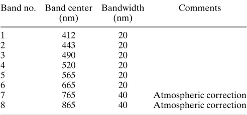
6 665 20
7 765 40 Atmospheric correction 8 865 40 Atmospheric correction
Table 4 OCTS thermal bands (µm)
[image:9.594.41.289.646.742.2]August 1997, over 10 years after the demise of CZCS. It is now in orbit and providing very high quality ocean color data. Unlike CZCS, it has no bands in the IR, so provides no information on SST (its successor MODIS will have IR bands, see section 3.1.4). A comparison of the capabilities of CZCS and SeaWiFS is given by Hooker et al..25/SeaWiFS flies on the SeaStar satellite operated by OSC, with NASA buying the data for distribution to the scientific community, while OSC sell the data to commercial organizations for other applications (see section 4.6).
SeaWiFS has six bands in the visible part of the electromagnetic spectrum and two bands in the near-IR for atmospheric correction purposes..27/ These bands are very similar to those of OCTS (compare Tables 3 and 5). The increased number of visible bands, plus the bands in the near-IR, and the improved sensitivity (see S/N in Tables 2 and 5) will allow better atmospheric correction of the data and improved retrieval of biological information, compared with CZCS..24/ SeaWiFS is a scanning instrument and has the capability to tilt š20° forwards or backwards to avoid sunglint. It is operated in two spatial-resolution modes, local area coverage (LAC) with a 1.1 km resolution at nadir, and global area coverage (GAC) with a 4.5 km resolution at nadir. At the nominal orbit altitude of 705 km, the LAC has a swath width of 2801 km, while the GAC has a swath width of 1502 km. The on-board recording system has only limited capacity for LAC data, so this capability is primarily for use when the satellite is within range of a ground receiving station.
3.1.4 Moderate Resolution Imaging Spectroradiometer
[image:10.594.304.551.128.363.2]MODIS is due for launch on the EOS-AM1 satellite in late 1999. Details of the instrument may be found in Barnes et al..28/ This instrument has 36 bands in the visible and IR part of the electromagnetic spectrum and will be used for atmospheric and terrestrial studies, as well as for biological oceanography. The bands and their uses are listed in Tables 6 and 7. At nadir, bands 1 and
Table 5 SeaWiFS bands
Band no. Band center Bandwidth S/N Comments (nm) (nm)
1 412 20 499
2 443 20 674
3 490 20 667
4 510 20 616
5 555 20 581
6 670 20 447
[image:10.594.305.551.396.618.2]7 765 40 455 Atmospheric correction 8 865 40 467 Atmospheric correction
Table 6 MODIS visible bands
Primary use Band no. Bandwidth Required (nm) S/N
Land/cloud 1 620 – 670 128 boundaries 2 841 – 876 201 Land/cloud 3 459 – 479 243 properties 4 545 – 565 228 5 1230 – 1250 74 6 1628 – 1652 275 7 2105 – 2155 110 Ocean color/ 8 405 – 420 880 phytoplankton/ 9 438 – 448 838 biogeochemistry 10 483 – 493 802 11 526 – 536 754 12 546 – 556 750 13 662 – 672 910 14 673 – 683 1087 15 743 – 753 586 16 862 – 877 516 Atmospheric 17 890 – 920 167 water vapor 18 931 – 941 57 19 915 – 965 250
Table 7 MODIS IR bands
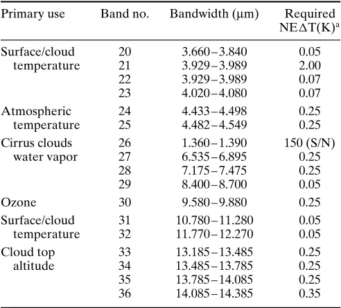
Primary use Band no. Bandwidth (µm) Required NET(K)a
Surface/cloud 20 3.660 – 3.840 0.05 temperature 21 3.929 – 3.989 2.00 22 3.929 – 3.989 0.07 23 4.020 – 4.080 0.07 Atmospheric 24 4.433 – 4.498 0.25 temperature 25 4.482 – 4.549 0.25 Cirrus clouds 26 1.360 – 1.390 150 (S/N)
water vapor 27 6.535 – 6.895 0.25 28 7.175 – 7.475 0.25 29 8.400 – 8.700 0.05 Ozone 30 9.580 – 9.880 0.25 Surface/cloud 31 10.780 – 11.280 0.05 temperature 32 11.770 – 12.270 0.05 Cloud top 33 13.185 – 13.485 0.25 altitude 34 13.485 – 13.785 0.25 35 13.785 – 14.085 0.25 36 14.085 – 14.385 0.35
a NET, Noise equivalent temperature difference.
[image:10.594.41.287.616.753.2]possible measurements the instrument has four on-board calibration systems (see Barnes et al..28/for details).
Although it was conceived as a two-instrument system (MODIS-T, with tilt capability, and MODIS-N, nadir looking), owing to cost constraints the tilting capability had to be foregone and a single instrument was designed. In order to compensate for the loss of oceanographic data due to sunglint (which could have been reduced using the tilt mechanism), a second MODIS instrument will be flown on the EOS-PM1 platform. It turns out that it is cheaper to design a single instrument and fly a duplicate, than to design and fly the original two-instrument system. The two instruments together will provide approximately the same global coverage as a single tilting instrument..9/ The MODIS capabilities for ocean observations are described by Esaias et al.,.9/ so only a brief summary is given here. It should be noted that MODIS’s ability to measure SST (using the IR bands), in addition to ocean color, will allow it to provide data on biophysical interactions. The end-result of the improved instrument performance is the ability to obtain more information on ocean biology. Basic information derived will concern the water-leaving radiance in the various bands. From these data information on pigment concentrations, chlorophyll-a, coccolithophores (see section 4.1.3), phycoerythrin (a specific algal pigment), ocean primary production (see section 4.1.2), and solar-stimulated chlorophyll fluores-cence will be obtained..9/MODIS will be the first satellite instrument to provide data on phycoerythrin and solar-stimulated chlorophyll fluorescence (see section 4.7.2).
3.1.5 Medium Resolution Imaging Spectrometer
MERIS.10/ is the ESA equivalent of NASA’s MODIS instrument described in the previous section, but without the bands in the IR part of the electromagnetic spectrum. It too will provide data for atmospheric and terrestrial, as well as oceanographic, studies (see Table 8). MERIS is a 15-band programmable instrument, so that the band positions and widths can in principle be changed during the mission. Only 15 of the 16 preliminary bands, listed in Table 8, will be acquired and transmitted when MERIS is in orbit. It will fly on ESA’s Envisat satellite at a nominal altitude of 800 km, giving it a swath width of about 1150 km, with 740 pixels across the swath. MERIS is a nontilting pushbroom type of instrument, so it will suffer from sunglint problems similar to MODIS.
[image:11.594.307.552.130.422.2]MERIS had been designed to be useful for both global and regional studies. For this reason it has two spatial resolution modes. The so-called full-resolution mode has a resolution of 300 m at nadir, while the reduced-resolution mode has a reduced-resolution of 1200 m at nadir, the latter being similar to CZCS, OCTS, SeaWiFS, and MODIS. The full-resolution mode is intended for regional
Table 8 MERIS bands
Band Band center Bandwidth Comments (nm) (nm)
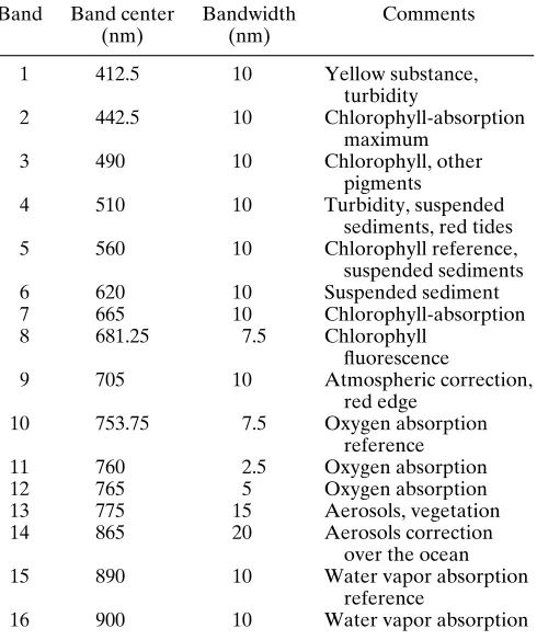
1 412.5 10 Yellow substance, turbidity
2 442.5 10 Chlorophyll-absorption maximum
3 490 10 Chlorophyll, other pigments
4 510 10 Turbidity, suspended sediments, red tides 5 560 10 Chlorophyll reference, suspended sediments 6 620 10 Suspended sediment 7 665 10 Chlorophyll-absorption 8 681.25 7.5 Chlorophyll
fluorescence
9 705 10 Atmospheric correction, red edge
10 753.75 7.5 Oxygen absorption reference 11 760 2.5 Oxygen absorption 12 765 5 Oxygen absorption 13 775 15 Aerosols, vegetation 14 865 20 Aerosols correction
over the ocean 15 890 10 Water vapor absorption
reference
16 900 10 Water vapor absorption
studies only, as the on-board data recording capacity is insufficient to capture all the data at this resolution on a global scale. Table 8 gives some indication of the types of information that will be derived from the various MERIS bands (see also Rast.10/). As with MODIS, particular care has been taken with the calibration systems for MERIS to ensure high quality of data.
3.2 Algorithms, Including Atmospheric Correction
As noted earlier (section 2), the critical measurement made by an ocean color sensor is the value of the water-leaving radiance Lw in each band in which the sensor measures. These measurements can then be related to the in-water biological constituents that are of interest to the biological oceanographer. The standard algorithms used to produce the global CZCS chlorophyll (pigment) concentration data set that is now widely available.6/are given by McClain et al..29/They are empirical algorithms that take into account the changes in the chlorophyll concentration. Thus the satellite-determined chlorophyll concentration Csatis given by Equations (5) and (6)
CsatD1.13
Lw.443/
Lw.550/ 1.71
and
CsatD3.33
Lw.520/
Lw.550/ 2.44
for 1.5 mg m 3<Csat. .6/ The change in algorithm at CsatD1.5 mg m 3is necessary as the value of Lw(443) becomes too small to quan-tify accurately at greater concentrations owing to the digitization and signal-to-noise characteristics of CZCS. The estimation of the near-surface pigment concentra-tion using these algorithms is accurate to within 35% for Case 1 waters..6/
The above algorithms are based on comparisons of the satellite data with in situ measurements and are therefore empirical in nature. More sophisticated algorithms have been developed for CZCS data that rely on modeling the dependence of the water-leaving radiance on the phytoplankton pigment concentration (for example, the so-called semianalytic model of Gordon et al..20/). In addition, regional algorithms have been developed to improve the retrieval of chlorophyll concentration in specific areas (for example, the Southern Ocean)..30/ These types of algorithm have not been applied routinely to CZCS data. The new generation of ocean color sensors, with more bands and improved digitization and S/N, will allow more sophisticated algorithms to be employed and more, and more accurate, biogeochemical information to be recovered from the data..9,24/
In order to obtain the water-leaving radiance values a simple atmospheric correction algorithm has been applied to the CZCS data set. A standard atmospheric aerosol type was assumed in order to correct for the presence of aerosols in the atmosphere..6/This correction introduces errors in regions where other types of atmospheric aerosol are present, such as off the north-west African coast, which is affected by Saharan dust. Other atmospheric correction algorithms have been developed and used for specific circumstances, some details of which have been given by Barale and Schlittenhardt..21/More sophisticated algorithms have been designed for the new generation of ocean color sensors (see, for example, Gordon and Wang.22/ for SeaWiFS and Gordon.16/ for MODIS). All the algorithms used for ocean color data have to screen the data to eliminate sunglint effects, and some of the more sophisticated algorithms take into account other effects that contribute to the radiances measures by the sensor, such as the presence of whitecaps on the sea surface. It is important to note that as the new generation of ocean color sensors have more radiometric sensitivity than CZCS, this in turn requires a better atmospheric correction algorithm if more accurate measurements of water-leaving radiances are to be made. The extra bands that the new sensors have allow for the atmospheric
correction procedure to be much improved over that used for CZCS..16/
The spatial and temporal coverage of the oceans pro-vided by CZCS was patchy. The data have been averaged to provide so-called higher level products, such as weekly and monthly composites. These can be used more eas-ily to study such phenomena as seasonal variations (section 4.1). Thus at Level 1 there are the individual CZCS images, with calibrated radiances, having a spatial resolution of 1 km. At Level 2 there are the derived geophysical parameters for each CZCS images, at a 4 km spatial resolution, the derived parameters being the phytoplankton pigment concentration, the diffuse atten-uation coefficient, normalized water-leaving radiances at 440, 520, and 550 nm, and the aerosol radiance at 670 nm. At Level 3, the data have been binned onto an Earth-grid with about an 18.5-km resolution at the equator. The Level 3 data are available as daily, weekly (5 days) and monthly averages. Full details of these data are given by Feldman et al..6/ SeaWiFS and OCTS data are now becoming available in similar formats over the Internet.
3.3 Calibration and Validation
The calibration and validation of spaceborne ocean color sensors is vital if the data obtained are to be used in any quantitative manner, rather than just as images of the sea. Considerable effort has been and will continue to be devoted to the calibration and validation of the data from ocean color sensors. Particular emphasis on the quality of the atmospheric correction applied to the data is necessary, as this has such a large impact on the retrieved water-leaving radiance values that provide the basic input into all the bio-optical algorithms..8/ As noted in the previous subsection, if the improved radiometric sensitivity of the new sensors means that a better atmospheric correction be applied to the data, this in turn will need to be validated..31/
must be taken to make measurements across a range of conditions for the calibration and validation process to be successful and useful. A further consideration is the temporal and spatial sampling of the in situ measurements compared with those made by the satellite. Clearly a ship can survey only a small part of an area that the satellite can see instantaneously, and in the time it takes to carry out the survey conditions may have changed (for example, owing to the currents advecting the phytoplankton around). Similarly how representative are data measured by a buoy at a single point, compared with the typical 1-km square pixel measurement obtained by the satellite, given the spatial variability of the phytoplankton?
The end-result of the calibration and validation efforts for the CZCS global data set was that the accuracy of the pigment concentration retrieval was shown to be 35% in Case 1 waters, and within a factor of two otherwise..6/ The aim for SeaWiFS is to obtain water-leaving radiances to within 5% and chlorophyll-a concentration to within 35% across the range 0.05 – 50 mg m 3..25/To achieve this a comprehensive calibration and validation plan has been adopted..32/ Similar procedures are being adopted for the other ocean color missions.31/ and should provide well-calibrated data for use in scientific studies.
4 APPLICATIONS
The previous sections have given some indication of the complexity of obtaining biological information from remotely sensed ocean color measurements from space. In this section the focus will be on how such measurements may be used to improve our understanding of biological oceanography. All the examples that will be discussed rely on the use of CZCS data. Although OCTS and SeaWiFS have provided and are providing new ocean color data (see section 2), little has yet appeared in the open literature on the application of these data to the study of ocean biology. In addition to scientific applications of the data, which will be the main focus of this section, the commercial applications of the data will also be briefly discussed, as will potential future scientific applications of data from the new generation of ocean color sensors (MODIS, MERIS).
Before proceeding it is useful to define and discuss a number of terms that will be used in this applica-tions secapplica-tions..5,13,17/The growth of phytoplankton in the upper layers of the ocean is controlled by the availability of sunlight and nutrients (such as nitrate, silicate, phos-phate, and iron) and by predation (the algae being eaten by zooplankton). In general, the phytoplankton may be regarded as passively advected by the turbulent flow in the ocean surface layer, the so-called mixed layer. A
phytoplankton bloom occurs when the factors affecting growth are such that rapid growth can occur. For example, blooms may be caused by the injection of nutrients into the mixed layer due to the presence of a cyclonic eddy, which causes local upwelling of nutrient-rich water..33/ The spring bloom occurs in certain parts of the ocean (for example the North Atlantic Ocean) when the mixed layer, deepened by the effects of winter storms, begins to shallow as the ocean begins to heat up in the spring (a process known as restratification). The mixing down of the layer in winter has entrained fresh nutrients into the layer. It has also reduced phytoplankton growth as the phytoplankton have been mixed down by the turbulence in the layer away from the euphotic zone. The shallowing of the layer in spring means that the phytoplankton spend more time in the euphotic zone, allowing them to grow rapidly (abundant sunlight and nutrients). At this stage predation is low because zooplankton numbers are low, so phytoplankton growth outstrips zooplankton grazing and a bloom occurs. As the zooplankton begin to grow rapidly and grazing increases, and the phytoplankton use up the nutrients in the mixed layer, growth begins to slow and then the numbers decay owing to mortality and predation. The zooplankton numbers then decrease (owing to lack of food) and by late summer the bloom has finished. This cycle is repeated each year. Various variations of this cycle are possible, but will not be dis-cussed here (see, for example, Mann and Lazier.5/ and Longhurst.17/). Regions of the ocean that have low con-centrations of the nutrients required for phytoplankton growth are called oligotrophic, while those that have high nutrient concentrations are called eutrophic. Many of the nutrients necessary for phytoplankton growth (such as CO2) are available in the ocean in sufficient quanti-ties not to limit growth. The key nutrients necessary for phytoplankton growth that may only be available in low concentrations, and therefore limit growth, are nitrate, sil-icate, and phosphate (sometimes called macronutrients). In addition, small quantities of so-called micronutrients (trace elements such as iron) are also necessary for the growth of some species of phytoplankton. Ocean areas where phytoplankton growth is limited by lack of iron or some other process (such as grazing by zooplankton), but that have an abundance of the macronutrients are called high nitrate (or nutrient) low chlorophyll (HNLC) areas.
4.1 Measurements of Phytoplankton
primary production, and of coccolithophores (a particular type of phytoplankton). The examples discussed are illustrative rather than comprehensive; other information may be found in the reviews of Abbott and Chelton.34/ and Aiken et al..24/
4.1.1 Chlorophyll and Other Pigments
As discussed earlier (section 2) ocean color measure-ments give information about the phytoplankton present in the near-surface layers of the ocean due to the pres-ence of chlorophyll-a and other pigments necessary for photosynthesis in the phytoplankton and to associated colored degradation products from the phytoplankton. Thus the basic information provided from the ocean color sensor is a measure of the surface concentration of chlorophyll-a and associated pigments. Relating this con-centration to the phytoplankton is a nontrivial exercise,.11/ but the satellite chlorophyll concentration measurements in themselves have provided a unique insight into the global biological behavior of the oceans.
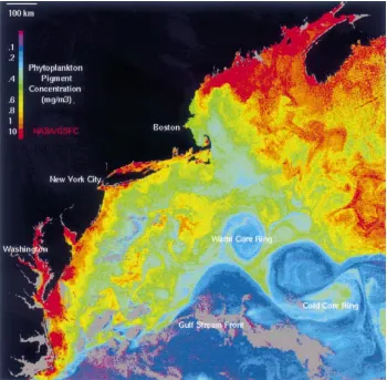
Perhaps the simplest observation that has been made has arisen from producing seasonal (spring, summer, autumn, winter) pictures of the global chlorophyll con-centrations derived from CZCS data (see, for example, McClain et al..29/ and Figure 1). These pictures show: (1) the occurrence of the spring bloom in the North Atlantic, (2) the relatively constant biological behav-ior of the Southern Ocean, (3) the low-concentration (desert-like) regions of the subtropical gyres, (4) the high concentrations in the Arabian Sea during the sum-mer monsoon, and (5) the higher concentrations in the northern and tropical Atlantic compared with equivalent regions of the Pacific Ocean. The reasons for these phenomena are related to the ocean physics and will be discussed below (section 4.3). The point to note here is that, while these phenomena had been observed previ-ously from scattered ship-based observations, CZCS data on chlorophyll concentrations provided the first global and spatially coherent view of them.
Yoder et al..35/ have used the monthly CZCS chloro-phyll concentration values to look at the biological seasonal cycle in the oceans on a global scale. They averaged the data spatial into latitude bands, defining an equatorial band and northern and southern hemisphere subtropical and subpolar bands. Despite some prob-lems associated with the coverage available from CZCS data, fewer data having been acquired in the southern hemisphere than in the northern, they were able to compare the seasonal changes in the chlorophyll con-centration for the Atlantic, Pacific, and Indian Oceans in the appropriate latitude bands. They found that the coverage of the equatorial Atlantic Ocean was poor and concluded that the annual cycle, with a maximum in
December, may not be representative. For the equato-rial Pacific Ocean they found no seasonal cycle, while for the equatorial Indian Ocean they concluded that the maximum in August/September is related to the subtrop-ical monsoon cycle there. For the subtropsubtrop-ical Atlantic and Pacific Oceans, they found that the seasonal cycles are similar, with the winter chlorophyll concentrations approximately double those of the summer. This pat-tern was attributed to the higher nutrient flux into the mixed layer in winter and the relatively high solar irra-diance during winter (compared with higher latitudes). The subtropical northern Indian Ocean was found to be anomalous, with the highest chlorophyll concentra-tions in the summer months. This was explained by the upwelling of nutrient-rich waters during the summer mon-soon. For the subpolar waters of the North Pacific and North Atlantic Oceans they found the existence of the spring bloom, which was more pronounced in the North Atlantic Ocean. This bloom is the result of the increase in solar irradiance in the spring, the shallowing of the mixed layer (due to solar heating and restratification) and the corresponding growth in phytoplankton. This growth outstrips the zooplankton grazing rate initially, but by late spring or summer the phytoplankton losses are greater than their growth and the bloom declines. The subpolar waters of the southern hemisphere were found not to exhibit this pattern. This hemispherical asymmetry may be due to differences in micronutrient (iron) availability, solar irradiance, vertical mixing, or zooplankton grazing. Overall, the seasonal patterns found by Yoder et al..35/ are consistent with predictions based on simple models of predator – prey (zooplankton – phytoplankton) interac-tions with implicit assumpinterac-tions about growth limitation by nutrients and solar irradiance. In some respects this agreement is surprising as there is considerable spatial and temporal variability in the distribution of phytoplankton (section 4.3). Therefore the averaging procedure used.35/ might have suppressed or distorted any seasonal signal, which it has not. Instead, their results confirm on the large scale a picture of the seasonal behavior of the phytoplank-ton that was arrived at originally from a more limited set of in situ observations. Banse and English.36/have given a complementary view of seasonal cycles which focuses more on specific areas and considers interannual variabil-ity. Their results are in broad agreement with those of Yoder et al.,.35/but show more regional detail as they did not use latitudinal averaging.
(a)
.1 .2
.4
.6 .8
10 1
(b)
.1 .2
.4
.6 .8
10 1
(c)
.1
.2
.4
.6 .8
10 1
(d)
.1
.2
.4
.6 .8
[image:15.594.128.467.107.664.2]10 1
Figure 1 (a) CZCS seasonal sea surface chlorophyll distribution for the northern hemisphere winter months, using data from 1979 to 1986. Note that the color scale is logarithmic in chlorophyll (phytoplankton pigment) concentration (units of mg chlorophyll m 3).
They found that blooms were localized to three regions: (1) in shallower waters (near continental margins, islands, and over shoals), (2) in coastal polynyas of the Antarc-tic sea ice zone, and (3) downstream of the continents (South America, Africa, Australia plus New Zealand) that interrupt the flow of the major circumpolar currents. In relation to the blooms downstream of the continents, they conclude that transport of iron (thought to be the limiting micronutrient in the Southern Ocean) from the adjacent continental shelves stimulates and sustains these blooms. They provide evidence of latitudinal banding of the chlorophyll concentration around the Antarctic con-tinent and link this to the physical processes that occur there. The results obtained.30/ are now being used in conjunction with other observations to study the ecology of the Southern Ocean..37/ This shows that the CZCS data are both of intrinsic interest and of value in gaining a better understanding of the ecology of the oceans, in combination with other data. This points the way forward for the use of the new ocean color data that are being and that will be acquired.
Many other examples of the use of chlorophyll concentration data from CZCS could be given; the ones given have been chosen to illustrate the unique value of remotely sensed ocean color data and their potential for understanding the biology of the oceans.
4.1.2 Primary Production
Phytoplankton are the main primary producers of the upper ocean, in that they convert inorganic compounds (nutrients, such as nitrate and silicate) into organic compounds through photosynthesis. This is the beginning of the oceanic food chain and the amount of organic material (biomass) produced is known as the primary production..13/ The rate at which biomass is produced is known as the primary productivity. The net primary production takes into account losses due to respiration and is the amount of photosynthetically fixed carbon available to the next level in the food chain..38/ The primary production may further be subdivided into new and regenerated components. New production is that based on new nutrients that have entered the euphotic zone, while regenerated production is that which occurs due to the recycling of nutrients there (through processes such as microbial breakdown of dead organic matter and fecal pellets). The ratio of new to total primary production is known as the f -ratio..39/Understanding the oceanic primary production is important for the carbon cycle and the CO2 problem (see section 4.2). It is also important in terms of assessing the sustainability of the global fisheries,.40/ an increasingly vital issue given the increasing world population’s requirements for food.
In order to estimate primary production it is necessary to have not only the surface chlorophyll information
from ocean color data, but also information about the photosynthesis – light relationship and possibly the structure of the chlorophyll distribution in the vertical. Here two recent attempts to estimate the primary production of the oceans from CZCS data are described, those of Longhurst et al..39/and Field et al..38/References to earlier attempts may be found in these papers.
Longhurst et al..39/ use chlorophyll estimates from CZCS and an approach developed by Platt and Sathyendranath.41/to calculate primary production. They divide the ocean up into a number of biogeochemical provinces, based on in situ and satellite data, in order to specify the spatial and temporal variability of the param-eters that are needed by their algorithm for primary production. The provinces are an attempt to characterize the biological, chemical, and physical variability of the oceans. As well as the surface chlorophyll value from CZCS, their algorithm requires information about the depth of the chlorophyll maximum, the standard deviation around the peak value, and the ratio of the chlorophyll peak at its maximum to the total peak biomass. The latter information is compiled from an extensive database of ship-based observations. From this information a vertical chlorophyll profile is constructed at each point on a global 1°grid on a quarterly basis (centered on the 15th day of January, April, July, and October). The calculations were restricted to a quarterly basis owing to the sparsity of in situ measurements available. Surface radiation was com-puted from the sun angle and climatological information from cloud cover. This was combined with experimentally derived information on the photosynthesis – light rela-tionship, representing polar, westerlies, trade-wind, and coastal domains, to calculate the total primary produc-tion. The calculation makes no allowance for the presence of suspended sediments in coastal waters for which the CZCS chlorophyll algorithm is inadequate and which will affect the estimates obtained. Taking this and other uncertainties into account and integrating over the year, Longhurst et al..39/estimate the annual primary produc-tion as 44.7 – 50.24 Gt C per year (1 Gt C is one Gigatonne of carbonD1 Pg C, one Petagram of carbonD1015g of carbon). They found that this figure is in reasonable agreement with extrapolations based on a few good in situ measurements.
This model is based on the work of Behrenfeld and Falkowski,.43/who suggest that the improvement gained by using a vertically resolved model, such as that of Longhurst et al.,.39/ is negligible compared with using a depth-integrated model. Their resulting estimate of global net primary production is 48.5 Gt C per year, which lies in the middle of the range calculated by Longhurst et al..39/It is interesting to note that while the production is of the order of 50 Gt C per year, the actual phytoplankton biomass is only ca. 1 Gt C. This implies that the phytoplankton biomass turns over approximately once per week on average..44/This is consistent with the fact that the phytoplankton lifecycle is relatively short, of the order of a day.
Prior to the availability of ocean color data, estimates of global primary production were more difficult to obtain..39,44/ Both of the approaches discussed above rely on more than just the satellite data to obtain these estimates. Neither method is able to distinguish between new and regenerated production, which it is necessary to do in studying carbon fluxes into the ocean (section 4.2). However, Sathyendranath et al..45/ have proposed a method for doing this using satellite data (see section 4.2 below). Algorithms for estimating primary production are being developed for MODIS..9/
4.1.3 Coccolithophores
Coccolithophores are phytoplankton that form external calcium carbonate CaCO3scales called coccoliths, which are a few micrometers in diameter and ca. 250 – 750 nm in thickness. These can form multiple layers, which even-tually detach and sink to the sea floor. Coccolithophores are also one of the principal producers of dimethyl sulfide (DMS)..46/ Their importance is probably greatest dur-ing a bloom, where their concentrations can reach up to 115 million cells per liter..47/ The most abundant of the species is Emiliania huxleyi, which can be found through-out most of the world’s oceans, with the exception of the polar oceans..48/ They can be detected in satellite imagery because the presence of the coccoliths leads to high reflectance in the surface waters due to their intense scattering of light..47/Essentially they act like small mir-rors suspended in the water and cause a significant portion of the incoming light to be reflected back out from the water.
Whereas phytoplankton pigments change the water-leaving radiance differential across the spectrum owing to absorption, coccolithophore blooms tend to increase the radiance uniformly owing to scattering..9/ The resulting appearance of the ocean can be milky, which is how these blooms were first observed by eye. A consequence of this is that coccolithophore blooms can be detected using the visible channels of the AVHRR, which are
not sensitive enough for studying other changes in ocean color..48/ Another consequence is that, in the case of ocean color sensors, a different algorithm needs to be used to estimate their abundance from satellite data..47/It also means that it is possible to monitor one specific species of phytoplankton, whereas the standard chlorophyll measurements obtained from ocean color do not allow discrimination between different species of phytoplankton. Two effects of the presence of large numbers of coccoliths in the water are first, an increase in the ocean’s albedo, and, second, a shading effect that reduces the light level in deeper water (while the scattering of photons increases the light level in the surface waters). These effects have not been studied using satellite data to date (1999).
The most comprehensive study of coccolithophore blooms in the global ocean using ocean color data, from CZCS, is that of Brown and Yoder..47/ They mapped the distribution of blooms using CZCS five-day composite normalized water-leaving radiance data from 1978 to 1986. The data used have a spatial resolution of 20 km. An automatic spectral classification scheme was used to detect the blooms, based on the spectral characteristics that have been obtained from in situ measurements. Monthly and annual composites were calculated from the five-day composite analyses. They found that coccolithophore blooms annually covered an average area of 1.4ð106km2 of the global ocean from 1979 to 1985. This represents ca. 0.5% of the ocean surface. Blooms were most extensive in the subarctic North Atlantic Ocean, annually covering an area of 105km2 (approximately equivalent to the size of England). As the scattering of light is due to the presence of coccoliths in the water, rather than of the cells themselves, the results are biased towards the declining stage of the blooms when the proportion of coccoliths to cells is greatest. Based on these results they were able to make estimates of CaCO3 and DMS production, using further assumptions regarding the depth of the mixed layer and the concentrations of cells and related chemicals within it. They concluded that on a regional scale the blooms are a significant source of CaCO3 and DMS. In contrast, on a global scale, the blooms detected in CZCS imagery play only a minor role in the production of CaCO3and DMS and their flux from the mixed layer to deeper waters and to the atmosphere, respectively.
4.2 The CO2Problem
imbalance between the atmosphere and ocean that allows the ocean to absorb CO2 from the atmosphere. Most of the CO2 removal is not permanent. Approximately 90% of the phytoplankton die and are decomposed in the surface waters rereleasing their CO2. The remaining fraction (ca. 10%) sinks down into the deeper ocean where it remains out of contact with the atmosphere for long periods of time (as much as 1000 years). A very small fraction (−1%) reaches the sea floor where it becomes part of the sea floor sediments and is therefore totally removed from the system (on timescales shorter than geological ones, that is millions of years)..49/Ocean color measurements have been used to look at two parts of this process, the transfer of gases between atmosphere and ocean, and the so-called biological pump that removes the CO2to the deep ocean and sediments.
4.2.1 Air – Sea Gas Transfer
The air – sea transfer of gases is dependent on many com-plex processes including wave breaking, the production of droplets and spray, the entrainment of air bubbles into the water and their subsequent behavior, and the pres-ence or abspres-ence of surfactants. Clearly this complexity is too difficult to model in all its aspects. Therefore the net air – sea flux of CO2is usually parameterized in terms of a wind speed-dependent gas exchange coefficient mul-tiplied by the difference in the partial pressure of CO2 (pCO2) in the air and in the water..50/ The presence of phytoplankton in the surface waters of the ocean, which use the CO2for photosynthesis, decreases the pCO2of the surface waters allowing greater uptake of CO2from the atmosphere. At the present time the potential feedback (whether positive or negative) between changes in climate (increasing atmospheric CO2) and the phytoplankton are not understood..1/
In situ measurements in the North Atlantic Ocean.51/ have shown that the spatial variability of the oceanic pCO2 is correlated with the spatial variability of the SST and chlorophyll concentration. These results were obtained in the springtime, during the bloom period. Watson et al..51/ suggest that using satellite-derived SST and chlorophyll values may allow the determination of the pCO2 value. Subsequent modeling studies by Antoine and Morel.52/ (see also Antoine and Morel.53/) have shown that the relationship between pCO2, SST, and chlorophyll varies spatially and temporally, but may be sufficiently stable on a seasonal basis to make a pCO2 estimate based on satellite data. To date (1999) this does not appear to have been done.
However, a related study has been carried out by Erick-son and Eaton,.54/who studied the flux of carbonyl sulfide from ocean to atmosphere, using CZCS data and an ocean general circulation model. The CZCS chlorophyll
data are related empirically to the maximum potential carbonyl sulfide concentration in the surface ocean. The assumption is that the chlorophyll data are representative of the maximum supply of organosulfur compounds that are available for photooxidation. The maximum potential concentration is then related to the actual concentration taking account of the surface radiation field of the ocean. Using an appropriate gas transfer coefficient (see above and Liss and Merlivat.55/) and information on surface radiation, the wind field, and SST, Erickson and Eaton.54/ calculate the gas flux for a five-year period, with a 2.8° spatial resolution, and a 24-hour temporal resolution. Computed values of surface concentrations of carbonyl sulfide are said to agree with experimental data on a regional basis to within the uncertainties of the calcula-tion. They found two orders of magnitude variation in the spatial and temporal gas flux, with the comment that the technique is potentially extendible to other biogeochem-ically important gases, such as CO2.
To conclude this section, it is worth noting that the gas transfer coefficient itself may be estimated from satellite scatterometer or passive microwave radiometer data on the oceanic wind field. Etcheto et al..56/have used passive microwave radiometer wind speed data and the Liss and Merlivat.55/ formulation of the transfer coefficient’s dependence on wind speed to do this. They show that the seasonal variations are large and need to accounted for in calculating the flux of CO2. Together with satellite-based SST and chlorophyll measurements, this provides the basis for global calculation of the air – sea flux of CO2 and other biogeochemically important gases.
4.2.2 Biological Pump