Lot streaming and batch scheduling: splitting and grouping jobs to improve production efficiency

Full text

(1)University of Southampton Research Repository ePrints Soton. Copyright © and Moral Rights for this thesis are retained by the author and/or other copyright owners. A copy can be downloaded for personal non-commercial research or study, without prior permission or charge. This thesis cannot be reproduced or quoted extensively from without first obtaining permission in writing from the copyright holder/s. The content must not be changed in any way or sold commercially in any format or medium without the formal permission of the copyright holders.. When referring to this work, full bibliographic details including the author, title, awarding institution and date of the thesis must be given e.g. AUTHOR (year of submission) "Full thesis title", University of Southampton, name of the University School or Department, PhD Thesis, pagination. http://eprints.soton.ac.uk.

(2) UNIVERSITY OF SOUTHAMPTON. Lot Streaming and Batch Scheduling: splitting and grouping jobs to improve production efficiency. Edgar Possani. submitted for the degree of Doctor of Philosophy in Operational Research. Faculty of Mathematical Studies. December 2001.

(3) UNIVERSITY OF SOUTHAMPTON ABSTRACT FACULTY OF MATHEMATICAL STUDIES OPERATIONAL RESEARCH. Doctor of Philosophy L O T STREAMING AND BATCH SCHEDULING: SPLITTING AND GROUPING JOBS T O IMPROVE PRODUCTION EFFICIENCY. Edgar Possani This thesis deals with issues arising in manufacturing, in particular related to production efficiency. Lot streaming refers to the process of splitting jobs to move production through several stages as quickly as possible, whereas batch scheduling refers to the process of grouping jobs to improve the use of resources and customer satisfaction. We use a network representation and critical path approach to analyse the lot streaming problem of finding optimal sublot sizes and a job sequence in a two-machine flow shop with transportation and setup times. We introduce a model where the number of sublots for each job is not predetermined, presenting an algorithm to assign a new sublot efficiently, and discuss a heuristic to assign a fixed number of sublots between jobs. A model with several identical jobs in an multiple machine flow shop is analysed through a dominant machine approach to find optimal sublot sizes for jobs. For batch scheduling, we tackle the NP-hard problem of scheduling jobs on a batching machine with restricted batch size to minimise the maximum lateness. We design a branch and bound algorithm, and develop local search heuristics for the problem. Different neighbourhoods are compared, one of which is an exponential sized neighbourhood that can be searched in polynomial time. We develop dynamic programming algorithms to obtain lower bounds and explore neighbourhoods efficiently. The performance of the branch and bound algorithm and the local search heuristics is assessed and supported by extensive computational tests..

(4) Contents Acknowledgements. v. 1. Introduction. 1. 1.1. Background. 1. 1.2. Contributions. 2. 1.3. Organisation. 4. 2. Scheduling 2.1. 2.2. I 3. 5. Scheduling Machine Models. . . . . . . . . . . . . . . . . . . .. 6. 2.1.1. Single-Stage Environments. 6. 2.1.2. Multi-Stage Environments. 8. 2.1.3. Job properties. 9. 2.1.4. Objective Functions. 2.1.5. Model Notation. 12. 2.1.6. Dispatching rules. 13. . . . . . . . . . . . . . . . . . . .. Computational Complexity. 10. 18. Lot streaming. 22. Lot Streaming Basic Models. 23. 3.1. Introduction. 23. 3.2. Literature Review. 25. 3.3. Network Representation and Dominant Machines. 30. 3.4. A two-machine flow shop model. 34. I.

(5) CONTENTS 3.5 4. II 5. ii. Concluding Remarks. 39. Extended Models. 40. 4.1. Introduction. 40. 4.2. Lot streaming with sublot allocation. 41. 4.2.1. Preliminary results. 42. 4.2.2. Assigning one sublot efficiently. 44. 4.2.3. Sublot Allocation Heuristic. 53. 4.2.4. Complexity of Heuristic. 57. 4.2.5. Counterexample of optimality. .. 57. 4.3. Identical Jobs Multiple Machines. 60. 4.4. Concluding remarks. 66. Batching. 67. Combinatorial Optimisation and Batching Machine Scheduling. 68. 5.1. Introduction. 68. 5.2. Combinatorial Optimisation. 69. 5.3. Exact Solutions. 70. 5.3.1. Branch and Bound. 70. 5.3.2. Dynamic Programming. 72. 5.4. 5.5. Local Search Heuristics. 73. 5.4.1. Iterated Local Search. 76. 5.4.2. Simulated Annealing. 77. 5.4.3. Tabu Search. 78. 5.4.4. Genetic Algorithms. 80. 5.4.5. Neural Networks. 81. 5.4.6. Complexity of Local Search Heuristics. 82. The Batching Machine Model 5.5.1. 83. A batching machine model with restricted batch size to minimise the maximum lateness BMRS. 85.

(6) CONTENTS 5.5.2 5.6 6. iii Solution for the unrestricted batch size model. Concluding Remarks. 86 . 87. Branch and Bound for BMRS problem. 89. 6.1. Introduction. 89. 6.2. Preliminary Results. 91. 6.3. Upper Bound. 93. 6.4. Branching Scheme. 94. 6.5. Lower Bound. 96. 6.6. Dominance Rules. 103. 6.7. Computational Experience. 109. 6.7.1. Experimental Design. 109. 6.7.2. Influence of Dominance Rules. 110. 6.7.3. Analysis of results. 112. 6.8. Concluding Remarks. 7 Local Search Heuristics. 115 117. 7.1. Introduction. 117. 7.2. Classical Neighbourhoods. 118. 7.3. Exponential Neighbourhoods. 121. 7.4. Split-Merge Neighbourhood. 123. 7.4.1. Neighbourhood Size. 124. 7.4.2. Merging Sequences. 125. Computational Experience. 126. 7.5.1. Test Problems and Experimental Design .. 126. 7.5.2. Comparing different splitting procedures. 127. 7.5.3. Comparing different neighbourhoods with a simple de-. 7.5. scent heuristic 7.5.4. Comparing different neighbourhoods with a multi-start descent heuristic. 7.5.5. 133 136. An iterated descent heuristic with the split-merge neighbourhood. 139.

(7) CONTENTS 7.6. iv. Concluding Remarks. 144. 8 Conclusions and Further Work. 146.

(8) Acknowledgements I would first like to thank my supervisor, Prof. Chris N. Potts, for all his help and time; without his support and guidance this work would have never been done or written. His fine intuition, broad knowledge, and work capacity have always been an inspiration to me. I would also like to thank Dr. Celia A. Glass, who was my supervisor for the first half of my PhD. Had it not been for her I would probably not have started my studies at the University of Southampton. It has been an enriching experience to do research with both of them. I was funded by Consejo Nacional de Ciencia y Tecnologia (CONACYT 115925) throughout my studies, and was a grateful recipient of the Postgraduate Overseas Scholarship from the Faculty of Mathematical Studies. I am in debt to both institutions for allowing me the opportunity to study in this country. If anything, I will take with me very fond memories of all the people I have met throughout these years. I would like to thank: Richard, Jon and Marta, who shared an office and a common research area with me, they kept me company in what is sometimes a very lonely experience; Pablo, Richard, Tom, Catherine and Eva for all the fun time we spent (and spend) together outside the Faculty; special thanks to Carla, Spiros, Paul, and Marta for sharing the same roof with me; and all the others who I have not mentioned, but made my stay in Britain a delightful experience. I would also like to thank Yvonne Oliver and Pat Taylor for all their help and kindness, they always made a visit to the fifth floor a fun trip; and Peter Hubbard for help with computing facilities. Thanks to my family for being close and always present: all the e-mails and phone calls kept me going; also to my aunt Lorena for making my first Christmas away from home a bit more bearable. "La tercera es la vencida", once again, thanks to Marta, I would not have finished this thesis without your love, never-ending patience, help and encouragement. Te quiero cosita..

(9) Chapter 1 Introduction 1.1. B ackgr ound. Activities that transform resources into goods and services, that take place in all sorts of organizations, are of interest to production and operations management. Efficient decision making at this level is important in increasing productivity as pointed out by Heizer & Render (1996). Scheduling plays an important role in production planning for manufacturing, and in increasing its efficiency, more so with the advent of computers and automated systems. However, its uses are wider, and many applications can be found outside manufacturing and production in the service industries area. In the competitive environment of today, efficient scheduling has become a necessity for survival in the marketplace. This thesis deals with issues arising in manufacturing, in particular related to production efficiency. The problems we consider are scheduling problems. Scheduling deals with the allocation of scare resources (machines) over time to tasks (jobs). We concentrate in two different areas: lot streaming and batching. Lot streaming refers to the process of splitting jobs, where as batching refers to the process of grouping them. Both are common processes in manufacturing, and are of considerable interest, as can be seen by an extensive literature..

(10) CHAPTER 1. INTRODUCTION. 2. Lot streaming is motivated by a desire to move the production of a job through several work stations or stages as quickly as possible. It can be considered an extension on the classical models in scheduling theory, where jobs are processed fully on a machine before continuing to another stage in the system, for in this case partially completed parts of a job are passed to downstream machines. Our aim was to show the advantages of network representations for the models, like the ones presented in Glass & Potts (1998), to obtain new results for the flow shop environment. Research on lot streaming was done under the supervision of Dr. Celia A. Glass. Most batching problems arise from the effort of grouping similar jobs in order to reduce common setup times. However, in this thesis we are interested in modeling a batching machine, one which can process more than one job at a time. Applications can be found in the 'burn-in' operations in the manufacture of circuits boards, and for chemical processes that are performed in tanks or kilns. Our aim was to tackle the XP-hard problem of scheduling jobs on a batching machine with a restricted batch size to minimize the maximum lateness objective function. Research on batching was done under the supervision of Prof. Chris N. Potts.. 1.2. Contributions. The contents of this thesis are a result of work wholly carried out by the author while registered in postgraduate candidature at the University of Southampton. We now describe the main contributions of this thesis. Lot streaming A job is split into sublots, the question that most lot streaming models try to answer is that of finding optimal sizes for the sublots. Instead of using a linear programming approach we have used a network representation and critical path approach to analyse models in lot streaming, with good results. We have presented an alternative approach to analyse the lot streaming problem of finding optimal sublot sizes and job sequence in a two-machine flow.

(11) CHAPTER 1. INTRODUCTION. 3. shop with transportation and setup times. Our aim was to clarify and give more insight into the results given by Vickson (1995). We have also analysed extension of the models for the flow shop environment. In particular we have analysed the case where the number of sublots each job has is not predetermined. We are considering a situation where the number of sublots is a technological constraint for the whole schedule, rather than a particular one for each job, as is common in the literature. We present an algorithm to assign a new sublot efficiently, and discuss a heuristic to assign a fixed number of sublots between jobs. We have also analysed a model with n jobs in an m-machine flow shop with m > 3. The jobs have the same processing times and sublots on each machine. We have applied a dominant machine analysis to find optimal sublot sizes for jobs, and proven that the model reduces to a simpler single-job lot streaming problem.. Batching We have tackled the NP-hard problem of scheduling jobs on a batching machine with restricted batch size to minimise the maximum lateness. Our aim was to develop exact as well as approximation methods for this problem. We have designed a branch and bound algorithm for the problem. The performance of the algorithm has been assessed through extensive computational testing. We give dynamic programming algorithms to find lower bounds on the maximum lateness of a schedule with a restricted maximum batch size. We also developed local search heuristics for the problem. Different neighbourhoods have been designed and compared, one of which is an exponential sized neighbourhood that can be searched in polynomial time. We rely on dynamic programming algorithms to explore the neighbourhoods efficiently. Again, the development work is supported by computational tests. As far as the author knows these are the first algorithms, and heuristics developed for the problem. Potts & Kovalyov (2000) point out that there is little research done on branch and bound and local search for batching machine problems, and our aim is to fill part of this gap..

(12) CHAPTER 1. INTRODUCTION. 1.3. 4. Organisation. The thesis is divided into two main parts. Part I, deals with models in lot streaming while Part II is dedicated to the batching machine model. In Chapter 2, we give a brief introduction to the theory of scheduling, and computational complexity. We present the notation we will be using throughout the thesis. Chapter 3 gives an overview of the models studied on the lot streaming literature, and the techniques we are interested in applying. Here we present the alternative approach to schedule jobs in a two-machine flow shop. Chapter 4 looks at the extensions of the known lot streaming models. In Chapter 5, we talk about batching machine scheduling in the context of combinatorial optimisation problems. We explain techniques to find exact solutions (branch and bound, and dynamic programming), as well as approximate solutions (local search heuristics). We also introduce the problem we study in the two following chapters. In Chapter 6, we describe the branch and bound algorithm developed for the batching machine problem, and discuss the computational results obtained. In Chapter 7, we compare several local search heuristics over different neighbourhoods. We present a exponential size neighbourhood that can be searched in polynomial time.. Computa-. tional tests are used to compare the different methods. Finally Chapter 8 concludes the thesis, outlining potential further work..

(13) Chapter 2 Scheduling In this chapter we give a brief introduction to the theory of scheduling, and computational complexity. Our aim is to familiarise the reader with some scheduling problems and their models, and explain a general framework to classify the difficulty of solving them. We focus mostly on those concepts that are relevant to subsequent chapters. More elaborate introductions can be found for scheduling in Conway, Maxwell & Miller (1967), Baker (1974) French (1982), and Pinedo (1995). Scheduling problems go back to the beginning of the industrial era. However, the first samples of scientific analysis of such problems date back to the 1950's. The theory of scheduling is concerned with the efficient allocation of resources to tasks over time. For example, a resource may be a machine in a workshop, surgeons in a hospital, processing units in a computing environment, and so on. The corresponding tasks may be operations in a production process, the surgical procedures to be performed to patients, computer programs to be executed, etc. Each task and resource might have different properties, which need to be taken into account to do the allocation. The value of the allocation is usually expressed as a function of the completion time of the tasks, referred to as an objective function. The problem is then one of finding a minimum value for tins objective function. We introduce several models in Section 2.1. discussing popular objective functions.

(14) CHAPTER 2. SCHEDULING. 6. and properties of interest for the tasks and resources. We confine ourselves in this thesis to deterministic scheduling models (problems). That is, we assume the data that define the problem (tasks and resources) are known with certainty in advance.. 2.1. Scheduling Machine Models. The standard terminology in use is one set in a manufacturing environment, which reflects the beginnings of the theory. Hence, a task is referred to as a job, and a resource is referred to as a machine. Each job may consist of several operations. It is common to talk about n jobs to be scheduled on m machines, and usually a subscript j refers to a job, whereas the subscript i refers to a machine. It is sometimes useful to refer to the set of jobs or machines. The notation we use is J = {J\, J 2 , . . . , J n } , and M. = {M\- • • • •> Mm} for the set of jobs, and machines respectively. Thus, it is the same to refer to job j , or job Jj, likewise to machine i or machine Mt. Several models have been proposed, analysed, and classified in the literature. Classification schemes have been proposed based on different dimensions. There are two major dimensions that specify any model: the machine environment and the job properties. Machine environments are determined by the number of machines, how they are organised in the production system, and the way the jobs are processed through them. We can divide the machine environments into two broad classes single-stage and multi-stage environments. A single-stage environment corresponds to production systems requiring only one operation per job, whereas multi-stage environments correspond to production systems where there are jobs that require operations on different machines.. 2.1.1. Single-Stage Environments. Single-stage environments involve either a single machine or m machines operating in parallel. The single-machine model is the simplest one, where.

(15) CHAPTER 2. SCHEDULING. 7. jobs require one operation on the (single) machine. It is standard to consider a single machine as being able to processes just one job at at time. However, in this thesis we are interested in modeling a single machine that can process more than one job at a time: we call such a machine a batching machine (see Section 5.5). Single-machine models not only come from situations that are in their own right a single machine problems, but also arise as simplifications of more complex models. It is not uncommon that a single machine is a bottleneck in a complex production system, and thus the performance of the entire system depends on it. Single machine models are also important in decomposition approaches, where scheduling problems in complicated environments are broken down into a number of smaller, single machine scheduling problems, as simple rules to solve them are more common due to their simplicity. A parallel-machine system, is a generalisation of the single-machine model. In this case we have several machines that can process a job. It is common to distinguish between three settings: one where the m machines are identical, one where machines have different speeds, called uniform, parallel machines, and one where the machines are unrelated. In an identical parallel machine environment each job requires a single operation and it may be processed on any one of the machines. In a uniform parallel machine environment, any machine can process a job, but the machines operate at different speeds, where the speed does not depend on the job, but on the machine. This portrays the fact that some machines in the system might be older, and therefore operate at lower speeds (an obvious example is computers). In the unrelated parallel machine environment the speed of the machines not only differ from machine to machine, but also vary for different jobs on the same machine. For example, when machines represent people, then the processing time may depend on the job as well as on the person (machine). One person may excel in one type of job, whereas another person may specialize in another type of job..

(16) CHAPTER 2. SCHEDULING. 2.1.2. 8. Multi-Stage Environments. Multi-stage environments consist of several machines, where the jobs generally have more than one operation to be performed on the machine system. There are three main types of multi-stage environments: flow sh,op) open shop, and job shop. In a flow shop environment each job has to be processed on each one of the m machines (stages) in the same order. For convenience, we say the jobs pass through from machine 1 to m. All jobs have the same routing, and after processing on one machine they join a queue for the next. Jobs may be resequenced between machines. If no job changes order while waiting in the queue, then we refer to it as a permutation flow shop. In an open shop environment jobs have to be processed once on each of the m machines, but there is no restriction on the order any single job must pass through them. Hence, the routing becomes part of the allocation (decision) process. In a job shop each job has its own route to follow through the machines. The route is prescribed beforehand for each job and it can differ from job to job. It is assumed that each job visits each machine at most once. However, if we allow a job to visit a machine more than once, then the job shop is subject to recirculation. It is usual for a job to be processed completely at a stage before it is sent to the next stage. Nevertheless, there are cases when the operation on a job is stopped to be resumed later, or when partially completed work on a job is passed along to other stages (downstream machines). Specifically, some models allow job preemptions where the processing of a job j may be interrupted (preempted), to put a different job in the machine, and resumed at a later time. Preemption is motivated by a desire to implement appropriate priorities among jobs in a situation where two or more jobs compete for limited production resources. In fact we are splitting the operation of the job into smaller parts. Another case where splitting of jobs is allowed is lot streaming. However in this case the job processing is not necessarily interrupted by another job, but merely passed along to another machine in the system, while the processing continues on the job. Lot streaming.

(17) CHAPTER 2. SCHEDULING. 9. is motivated by a desire to move the production of the job through several work stations (stages) as quickly as possible. Sometimes jobs have precedence constraints, when certain jobs require the completion of some others before work can start on them.. 2.1.3. Job properties. The following are popular job properties, and we present the notation we will use for them throughout the thesis. • Processing time p^ of job j on machine i, is the time it takes for machine i to process job j . The subscript i is omitted if the processing time of the job does not depend on the machine, or if we are working with a single machine. Hence, for identical parallel machines p3 is the processing time on any machine, whereas in a uniform parallel machine environment the processing time of job j may be expressed as Pj/ui, where ui is the speed of machine i. • Due date dj of job j , is the time by which the job should be completed. In a manufacturing system it represents the committed shipping (or completion) date the job is promised to the customer. The completion of a job after its due date is allowed; however a penalty is incurred (usually expressed in the objective function). If the due date must necessarily be met then we refer to it as the deadline. • Release date r, of job j , is the time (date) at which the job becomes available for processing in the system. • Weight uij of job, which denotes the importance of a job relative to others; it is a priority factor. It might represent the actual cost of keeping the job in the system, such as a holding or inventory cost. Alternatively, it might just be a predefined value (cost) of the job. • Setup Sjjk time between jobs j and k on machine i. This may represent the clean up time after job j before job k starts processing on machine i..

(18) CHAPTER 2. SCHEDULING. 10. If the setups are not sequence dependent then we say srj is the setup time on machine i before job j starts. If the setup does not depend on the machine, or we are working with a single machine the subscript i is omitted. Sometimes similar jobs share a setup, we say they belong to the same family. If job k is processed immediately after job j on machine i and they belong to the same family, then szjk — 0. • Transportation time t^/, of job j between machine i and h, to represent the time it takes to transport job j from machine i to machine k. This property is inherent in multi-stage environments. If it is machine independent, or if the transport is always made in the same direction and only between two machines we may omit subscripts i and h. This can be viewed as a setup between machines for the same job, in a similar way to s ^ being one between jobs in the same machine. Note how some properties are predominantly time related like dj, and r.,, while some are also dependent on the job sequencing on the machines like s^k and tijk- Others are solely dependent on the job like uij, or are based on the particular environment where they are set such as preemption, lot streaming, or precedence constraints.. 2.1.4. Objective Functions. In scheduling terminology, a distinction is often made between a sequence, and a schedule. A sequence usually corresponds to a permutation of the jobs, that is, the order in which jobs are to be processed on a given machine. A schedule provides additional information, including the time that the operations occupy the machines and possibly some other features. For example, in an two-machine flow shop with lot streaming a schedule not only specifies the order the jobs go through both machines but the size of the sublots for each job (see Section 3.4). Once a schedule of the jobs is determined, we can calculate the completion time of each job. We will denote by Cj the completion time of job j . that.

(19) CHAPTER 2. SCHEDULING. 11. is the time the job leaves the system (i.e. its completion time on the last machine on which it requires processing). Sometimes it is useful to be able to refer to the completion time of an operation of job j on machine i, which we denote by Cij. As explained before, the objective function is usually expressed in terms of the completion time of the jobs. Some measures that can be calculated for each job and help define popular objective functions are: • the lateness of a job Lj = Cj — dj\ • the unit penalty Uj = 1 if Cj > dj, otherwise Uj = 0; • the tardiness Tj = max{Cj — dj, 0}; • the earliness Ej — max{<ij — Cj, 0}; • and the flow time Fj = Cj — Vj. Based on these measures we are able to calculate and propose the following objective functions. • Maximum completion time or makespan C max = max Cj. A minimum j. makespan usually implies a high utilisation of the machine(s). It is also a measure of the output rate of products in a system. • Total (weighted) completion time. ^2(WJ)CJ,. which gives an indication. of the holding costs incurred by the schedule. When Wj = 1 for each job j this objective function is equivalent to minimising the average number of jobs in the system, and is a measure of the average throughput time. • Total (weighted) flow time YKwj)^j. *s a similar measure to the previous. one, but this one considers the job release date. It allows for jobs entering the system at different times. Note that if r.y = 0 for all jobs j then.

(20) CHAPTER 2. SCHEDULING. 12. • Maximum lateness, L max = maxLj; this measures the worst violation of the due date. In some sense, minimising L inax is equivalent to minimising the worst performance of the schedule. • Total (weighted) number of late jobs J2 Uf. this is a common measure in practice, and easily recorded. It does not account for how late a job is, but just if it is late or not. However minimising this objective function may result in schedules where jobs are very late, which is often unacceptable in practice. • Total (weighted) tardiness. ^2{WJ)TJ;. this measures the conformance to. due dates, similarly to ^2(WJ)UJ, but it is less likely that the wait for any given job will be unacceptably long. • Maximum tardiness, Tmax, is similar to L max , but early jobs bring no reward. In this thesis we are interested in particular in the C max , and L max objective functions.. 2.1.5. Model Notation. The standard representation scheme for scheduling problems (Graham, Lawler, Lenstra & Rinnoy Kan 1979) is a three-field descriptor. V;I|V;2|V;3J. where ipi in-. dicates the machine environment, xp2 describes the job properties, and ip3 the objective function to be minimised. We let ^1 = « m, where m is the number of machines, and a e {P, Q, R, F, J, 0 } for identical, uniform, and unrelated parallel machines, flow shop, job shop and open shop environments, respectively. We use the notation suggested by Potts & Kovalyov (2000) where if the machines involved are batching machines we use tilde on top of the environment (for example, Pm is an identical parallel machine environment with m batching machines). Under ^2 we may have any of the job properties given above, and, or:.

(21) CHAPTER 2. SCHEDULING. 13. • hi if the maximum batch size on machine i is /;,;, and just b if the maximum batch size on all machines is h. • qj is number of sublots job j is allowed to have. When all jobs have the same number of sublots, we drop the index j . Models without lot streaming have q — 1, and there is no need to make it explicit in v 2 . • prec if there are precedence constrains, • pmtn if preemption is allowed, • recrc if recirculation is present in the system, Field ipa m a v be any of the objective functions explained before. For example, F2 \qj, Sij, tj\ Cmax is the two-machine lot streaming flow shop problem, minimising makespan, with sequence independent setup times s^-, transportation time t,, and q3 sublots for each job. This problem is solved in Section 3.4. Another example is J2 \bi = 1, b2 = 3| r m a x , a two machine job shop where the first machine is a classical machine, and the second is a batching machine that can process up to 3 jobs at the same time, minimising the maximum tardiness. In this thesis we study problem 1 \b\ Lmax, a single batching machine with restricted batch size to minimise the maximum lateness.. 2.1.6. Dispatching rules. A simple solution procedure for scheduling problems is to priorities jobs, and schedule them according to a dispatching rule. A dispatching rule prioritizes all the jobs that are waiting for processing on a machine. The prioritization scheme may take into account the jobs properties and machine attributes, as well as the current time. Pinedo & Chao (1999) distinguish between static and dynamic dispatching rules. These rules are usually constructive in their approach. A static rule prioritizes all jobs before constructing the schedule, and does not change the priority as the schedule is being constructed (i.e. it.

(22) CHAPTER 2. SCHEDULING. 14. is just a function of the data of the problem). Dynamic rules, on the other hand, are time dependent, and prioritize jobs differently with time as the schedule is constructed. The first results on the theory of scheduling were static dispatching rules that gave optimal solutions for some problems. As an example we present the following: • Shortest processing time (SPT) rule prioritizes jobs according to their processing time. It forms a schedule as a sequence of jobs in nondecreasing order of processing time. A schedule constructed in such a way minimizes the ^ C3 or ]T] vjjCj if Wj = w \/j in a single machine environment. This rule is also optimal for Pm\\ Y^ Cj, and Fm\prmu,pt3 C. Pj\J2 j. (. see. =. Pinedo (1995), Sections 4.3 k 5.1).. • Earliest due date (EDD) rule prioritizes jobs according to their due dates. It takes the jobs and orders them in non-decreasing order of their due dates to form the schedule as a sequence of jobs. It was proven by Jackson (1955) that this rule yields an optimal schedule for l||£max- We use it as well to construct starting solutions for our local search heuristics, see Chapter 7. • Shortest processing time first, largest processing time second (SPT(l)LPT(2)) rule, also referred to as Johnson's rule. This rule was originally designed for the i ? 2||C max problem, (Johnson 1954). It divides jobs into two sets; set 1 where the processing time on the first machine is smaller than the second (i.e. pX3 < p2j), and set 2 where the processing time on the second machine is smaller than on the first machine (i.e p\3- > p2j) Jobs where pij = p2j- may be in either set. The SPT(1)-LPT(2) rule dispatches jobs in the set 1 first, and in non-decreasing order of p\3, and dispatches jobs in set 2 afterwards, in non-increasing order of p2j. Another famous dispatching rule is the weighted shortest processing time first (WSPT) rule for 111 ]P iv3Cj, where the jobs are ordered in decreasing order of Wj/pj, due to Smith (1956). Several other dispatching rules.

(23) CHAPTER 2. SCHEDULING. 15. have been devised for different objective functions and environments (including O2, Jm, Fm); for a summary of other dispatching rules consult Pinedo (1995). Throughout the thesis we focus mainly on the C,nax objective function in a flow shop, and the L max objective functions on a batching machine. Hence, we are particularly interested in the SPT(1)-LPT(2) and the EDD dispatching rules. We now prove why these rules work. In particular Johnson's rule will be used extensively in Chapters 3 and 4. Theorem 2.1 (Johnson 1954). F2||C m a x is solved by an. SPT(1)-LPT(2). schedule. Proof:. Suppose that no optimal sequence corresponds to an SPT(l)-. LPT(2) schedule. In an optimal sequence, there is a pair of adjacent jobs, say h before I such that they satisfy one of the following 3 conditions: (i) job h belongs to set 2 and I to set 1: (ii) job h and / belong to set 1 and pnx > pu\ (iii) job h and / belong to set 2 and p2h < PnWe need to show that, under any of the three conditions mentioned above, by interchanging the positions of job h and / in the sequence we get a makespan that is shorter or the same. Let C,j denote the completion time of job j (1 < j < n) on machine i (i = 1, 2) under the original sequence and Cij the completion time under the sequence where h and / have been interchanged. Suppose that under the original sequence job t immediately precedes job h and that job g immediately follows job /. Interchanging h and / does not affect the starting time on the first machine of job g, which is equal to C\t + pm + Pu- However, we are interested in knowing when the second machine becomes available to process job g. Under the original sequence it is C2i, but with the interchange it is C2h- We need only to prove that, under any of the three conditions mentioned above. C>i, < C-j.i- The completion of job I on the second machine under the original sequence is C2i = max{max{C2(, Cn + pVl} + p2h,CH + pUl. + pv} + p2i =.

(24) CHAPTER 2. SCHEDULING. 16. = max{C2t + p2h + Viu Cu + plh + P2h + Pu-. Cu + V\i, + Pu and similarly the completion time of job h on the second machine after the interchange is C2h = max{C2t + P21 + P2h, Cu + pu + p2i + Pu,., Cu + Pu Under condition (i), p\h > p2h, and pu < p2i- Note that the first terms within the max expressions of C21 and C2/j are identical. The second term in the expression for C-ih is no greater than the third term in the expression for C21, and the third term in the expression for C2/1 is no greater than the second term in the expression for C21. Hence, under condition (/'), C2h < C<n. Under condition (ii), p\h < p2h as well as pu < p2i, and pu, > pu. In this case the second and the third terms in the expression for C?h a r e. n0. greater. than the second term in the expression for C2i- Hence, under condition (ii) C2/1 < C*2/.. Finally condition (iii) implies that pih > 7)2/1, and pu > P21, as well as P2/1 < P2i- So that the third term in the expression for C2i is no less than the third and second term in the expression for C2n • Hence under condition (iii) C2/1 < £2/- We need to repeat the same argument until we get an SPT(l)LPT(2) sequence. D Theorem 2.2 (Jackson 1955). l||L max is solved by an EDD schedule. Proof:. Let a be an optimal sequence, and Lnmx(a) its maximum lateness.. Suppose that no optimal sequence corresponds to an EDD schedule. Then there are at least two consecutive jobs in a say j sequenced before j' + 1 such that d(j) > d(j + 1). Construct a new sequence a' where job j + 1 is swaped with job j . The completion time of job j under o is C7_i +p 7 , and its lateness is Lj = Cj-i + Pj — dj, while the completion time of job j + 1 under a is Cj_i +pj+pj+i and its lateness L ?+ i = Cj-i+pj+pj+i. -dl+i.. Now consider. the maximum lateness of sequence a'. The lateness of each job before j and.

(25) CHAPTER 2. SCHEDULING. 17. j + 1 remains the same as no such job is affected by the swap. The lateness of each job after j and j + 1 also remains the same as the completion time of the job j in a' is Cj = Cj-\ + pj+i + Pj = C1+\. We only need to look a the lateness of jobs j and j + 1 under a'. The lateness of job j in a' is Lj. =. Cj-\ + pj+i + Pj — dj = Cj+\ — dj < Cj+\ — rij+i = Lj+i. and the lateness of job j + 1 in a' is LJ+\ = C3~\ +p y +i — fij+i. < L max (cr), <. Cj-± +Pj +. p i + i - dj+i = Lj+i < L max (a). Thus, Lmax(cr') < Lniax(cr). We can repeat the same argument until we get a sequence in EDD order.. • Dispatching rules, however, tend only to yield optimal solutions for simple models. We consider an algorithm to be a step by step solution procedure which yields an optimal solution to a problem. That is, an algorithm will construct an optimal schedule (i.e. one that minimises the objective function). A procedure that does not yield an optimal solution is referred to as a heuristic. We analyse a class of heuristics (local search heuristics) in Chapter 5, Section 5.4. General purpose algorithms like branch and bound, and dynamic programming are introduced in Chapter 5. Section 5.3. Many scheduling problems can be formulated as (mixed integer) linear programming problems MILP, see Schrijver (1986). Another solution procedure for scheduling problems, therefore, is the methodology for MILP problems. However, for most scheduling problems it is hard to find algorithms that solve them in a reasonable amount of time. It is common to classify the difficulty of scheduling problems by the time it takes to solve them. A frame for such a classification was introduced by Cook (1971) and Karp (1972), and is referred to as the theory of computational complexity. We give an overview of the theorv in the next section..

(26) CHAPTER 2. SCHEDULING. 2.2. 18. Computational Complexity. An intuitive way of classifying problems is the effort (time) required to solve them to optimality. The main contribution of the theory of computational complexity is .o give a framework for such a classification. In this section we give a non-rigorous overview of the concepts involved in this classification. For a rigorous and detailed treatment we refer the reader to the classical book by Garey & Johnson (1979). We also base our presentation on books by Papadimitriou & Steiglitz (1982), Papadimitriou (1994), and Cook, Cunningham, Pulleyblank & Schrijver (1998). An instance of a problem is obtained by specifying particular values for the parameters (machine environment, job properties) that define it. The size of an instance can be roughly defined as the number of symbols required to represent it. The effort (time) required for an algorithm to obtain a solution grows with the size of the problem instance. It is natural then, to represent this effort as a function of the size of the instance. In fact the running time of an algorithm for a given problem is measured by an upper bound on the number of elementary steps the algorithm has to perform. Specifically, if n is the size of an instance, and f(n) is an upper bound on the number of steps the algorithm performs, then the algorithm runs in O(g(n)) time, or is said to have O(g(n)) time complexity, if there exists a constant c > 0 such that for large enough n, f(n) < c g(n). An polynomial time algorithm is one where g{n) is a polynomial function. We have an exponential time algorithm, when it is not a polynomial time algorithm, this includes functions of the form n! and n'°s n . Other standard notation for the asymptotic running time of an algorithm (see Cormen, Leiserson & Rivest (1993)) is as follows. Let f(n) : Z+ —> K + and g(n) : Z+ —> 5R+ then f(n) is Q(g(n)) if there exists a constant c > 0 such that, for large enough n, f(n) > c g(n), and /(?;.) is Q(fj{n)) if there exist constants Q,c u > 0 such that, for large enough n, c\ fj(n) < f(n) < c. u g(n). Note that just as O-notation gives an asymptotic upper bound,. the Q-notation provides an asymptotic lower bound. We can use this same.

(27) CHAPTER 2. SCHEDULING. 19. notation to refer to the space requirement of the algorithm (information an algorithm needs to access while running), or to denote the size of a solution space (see Section 5.4). As explained before, complexity theory aims to classify problems into 'hard' or 'easy' depending on the time it takes to solve them. The core of the classification lies in grouping problems into two main classes, namely P and NP. The definitions of P (deterministic polynomial) and NP (nondeterministic polynomial) classes are based on the concept of a deterministic and non-deterministic Turing Machine. A Turing Machine is a mathematical model of an algorithm. A problem is in the P class if it is possible to solve it in polynomial time by a deterministic Turing Machine. A non-deterministic Turing machine is a theoretical extension of the deterministic machine which can evaluate an exponential number of solutions in a polynomial bounded number of computations. A problem is in NP if it can be solved in polynomial time by a non-deterministic Turing Machine. It follows that P C NP. In practice a problem belongs to class P if there exists an polynomial time algorithm that solves it. For example, the ellipsoid algorithm by Khachian (1979) solves any linear programming (LP) problem in polynomial time; hence LP problems belong to P. However, for a long time it was unknown if LP problems belonged to P. That there is no known polynomial algorithm for a problem does not guarantee that it does not belong to P, rather that the problem is intractable. However, it is of interest to know if such a problem is NP-complete. We note that the NP-completeness theory refers to decision problems (one whose solution is either 'yes' or 'no'). For any given problem there exists an associated decision problem. Membership of the NP-complete class is 'harder' to establish, and is based on the fact that all NP problems can be reduced to any NP-complete problem in polynomial time. Cook (1971) was the first to give an NP-complete problem, namely the satisfiability problem. If problem n can be reduced to problem IT by a polynomial time procedure, then they belong to the same class. This is significant because if we were able to find a polynomial time algorithm for.

(28) CHAPTER 2. SCHEDULING. 20. an NP-complete problem, then we would prove that P = NP. A list of NPcomplete problems can be found in Garey fc Johnson (1979), with recent results summarised in (Papadimitriou 1994). Unfortunately there has been no success in finding any polynomial algorithm for an NP-complete problem, nor in proving P ^ NP. In fact, what the theory seems to conclude is that the 'hardest' problems (NP-complete problems) are in some sense equivalent, and it is widely believed that NP ^ P. The size of an instance is encoding-dependent (i.e. dependent on the code or 'language' utilized to represent the parameters of the problem). NPcomplete problems, can be divided into two subclasses depending on the encoding scheme. These are unary NP-complete (or strongly NP-complete), and binary NP-complete (sometimes referred to as NP-complete in the ordinary sense). These concepts were introduced by Garey & Johnson (1978) and Lageweg, Lawler, Lenstra & Rinnooy Kan (1978). If a problem is unary NP-complete, then it is NP-complete even when the encoding scheme uses unary notation (where a string of n ones represents number n, expressed in base 1). Such a problem differs from a binary NP-complete problem by the fact that a binary NP-complete problem may have a pseudo-polynomial algorithm, one that runs in polynomial time if the encoding is unary. Hence, in some sense unary NP-complete problems are 'harder' than binary NPcomplete problems. Very informally a problem is termed unary NP-hard when the corresponding decision problem is NP-complete in the strong sense, and binary NP-hard if the corresponding decision problem is NP-complete in the ordinary sense. For a more detailed treatment of these terms (including Turing reducibility and number problems) consult Garey & Johnson (1979). In scheduling problems there is a thin line dividing NP-hard problems from P problems. For example, in problem lj|L niax , that belongs to P (as EDD rule solves it), changing to a batching machine with restricted batch sizes (i.e. l|6|Z/max) produces an NP-hard problem. Computational complexity is a worst case analysis, and is by no means a measure of the expected running time in practice. An illustrative example.

(29) CHAPTER 2. SCHEDULING. 21. is the simplex algorithm of (Dantzig 1949) that solves linear programming problems. It is an exponential time algorithm, but it works very well on average, and for many instances outperforms the ellipsoidal method. However, the theory does give an indication of the complexity of the problem, from which we can deduce the type of methods that are most suitable to find solutions. Heuristic methods, like the ones described in Chapter 5, are used for NP-hard problems if solutions are required using reasonable computational resources..

(30) Part I Lot streaming.

(31) Chapter 3 Lot Streaming Basic Models 3.1. Introduction. As explained in chapter 2, it is common for a job to finish its operation on one machine before proceeding to the next machine in the system. Lot streaming, however, is the process of splitting partially completed jobs into sublots to be transferred to downstream machines in multi-stage production systems. It is an extension on the classical machine models where the number of sublots for each job j , denoted by q3, is qj = 1. By allowing the overlapping between successive operations we may obtain a reduction on the completion time of the jobs in the resulting schedule, and the work-in-process inventory levels. Lot streaming also improves customer services, as partially completed sublots may be delivered before the whole job (order) is completed, as pointed out by Potts & Van Wassenhove (1992). We illustrate this in the following example. Consider the F2 | | C max model with 3 jobs, and the following processing times. Table 3.1: Processing times for a 3-job example job Jx h 4. 6. 6. 5. 8. 4. 23.

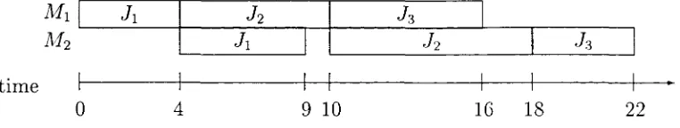
(32) CHAPTER 3. LOT STREAMING BASIC MODELS. 24. Johnson's SPT(1)-LPT(2) dispatching rule will give a schedule where job J\ is sequenced before J 2 , and job J2 before J 3 . with makespan C max = 22. A Gantt chart representing this optimal schedule is shown in Figure 3.1. Note how the operation on machine M\ for a particular job is finished before its operation on machine M2 begins. Machine M2 is idle for 4 time units before the operation on the first job starts, and it is idle for 1 time unit while it awaits for operation on job J 2 to finish on the first machine. J2. Jl. M2. Jl. J2. Jl. 1. Jl. time 4. 9 10. 16. 18. 22. Figure 3.1: Gantt Chart for the 3-job example Allow lot streaming on J 2 , say by dividing it into two equally sized sublots throughout the flow shop. Hence, divide the operation of J 2 on M\ in two 3 time unit sublots, and the operation on M2 in two 4 time unit sublots. The schedule with the same job sequence as before is shown in the Gantt chart of Figure 3.2. Note how for job J 2 there is an overlap of the operation on the second sublot on machine M\, and the operation of the first sublot on machine M2 (between time 9 and 10). Half of job ,72 (sublot 1) becomes available for dispaching to the customer at time 13, and the whole job is completed at time 17, whereas before its completion time was C 2 = 18. Not only that, but the duration of the whole process, the makespan of the schedule, is reduced to 21. This reduction in makespan results from a higher utilization of machine M2, where the idle time is reduced by 1 unit. My. Jl. M2. J 2 sblt 1 h sblt 2 Jz J sblt 1 J 2 sblt 2 2 Jl. •h. time 0. 7. 9 10. 13. 1011. 21. sblt = sublot Figure 3.2: Gantt Chart for the 3-job example, where q2 = 2.

(33) CHAPTER 3. LOT STREAMING BASIC MODELS. 25. A job may consist of several items. Hence, after they are completed in the first machine they wait until all of the items are finished before they move to the second machine. Those items waiting for others to be completed are part of the work-in-process inventory. We can appreciate how the inventory levels between time 4 and 10 are reduced when lot streaming is allowed. The aim of this chapter is to review important results for some models that deal with lot streaming, and give more insight into the F2 \qJ} s^, tj\ C max model. In Section 3.2 we give an overvie • of the results in the literature. In Section 3.3 we give more details on the network representation of the single job flow shop lot streaming model, and the dominant machine analysis by Glass Sz Potts (1998). In Section 3.4 we present a critical path approach to find an optimal schedule for the F2 \qv si3, tj\ C max model.. 3.2. Literature Review. Lot streaming models date back to work by Szendorvits (1975). His model shows that there are potential savings in the holding, work-in-process, and final inventory costs when lot streaming (overlap of operations) are considered in multi-stage production systems. His analysis focuses on a single job (production lot) with equally sized sublots. Goyal (1976) treats the problem of optimising the sublot sizes in Szendorvits model, both models assume there is no idle time between sublots (but there may be between different jobs). These results are in accordance with the just in time (JIT) philosophy where shorter production runs are preferred. The first lot streaming models focused in obtaining optimal sublot sizes for a single job. The makespan is a natural cost function, as the aim is to pass the lot (job) through the system as quick as possible. Baker (1988) gives a linear programming formulation for a single job in a flow shop environment, minimising the makespan. He allows idle time between sublots, and expresses the makespan as the sum of the idle times in the last machine plus the processing time of the sublots on that machine. His model assumes that the.

(34) CHAPTER 3. LOT STREAMING BASIC MODELS. 26. number of sublots is known (q fixed beforehand). One possible formulation for this problem focusing on the completion time of sublots, rather than the idle time is as follows. Lot streaming for a single job minimising the makespan Let Cki denote the completion time of sublot k (1 < k < q) on machine i (1 < i < m), and let Xk be the proportion of the job belonging to sublot k, then the problem of minimising the makespan of a single job with q sublocs through m machines can be formulated as: min Cgm subject to Cn -pixx. > 0,. Cki — Cki-i — PiXk > 0, for 1 < k < q, and 2 < i < m. (3.1). Cki — Ck-u — PiXk > 0, for 2 < k < q, and 1 < i < m. (3.2). x. ki Cki > 0,. for 1 < k < q, and 1 < i < m.. Note that Cqm is the completion time of the last sublot of the job in the last machine, which is the makespan of the single job. The processing time of sublot k on machine i is PiXk- Thus, the first inequality guarantees that the completion time of the first sublot on the first machine is not smaller than the processing time of the first sublot on the first machine. The set of inequalities (3.1) ensure that the processing of sublot k on machine i — 1 is completed before it starts its processing on machine i. This is usually referred to as the sublot processing constraint. The second set of inequalities (3.2) makes sure that sublot k — 1 has completed its processing on machine i before the processing of the next sublot (k) starts. This is referred to as the machine capacity constraints. The fourth inequality guarantees that Xk is a proportion of the job. A solution to this problem is fully determined by the values of Xk for k = 1,.. ., q. Baker (1988) showed explicitly that the sublot sizes for the two machine case (m = 2) are geometric. That is, if Xk is the proportion of the job.

(35) CHAPTER 3. LOT STREAMING BASIC MODELS. 27. belonging to sublot k then, (£2\fc-l Z. "= Y ^ ;. P-3). •. In general, let us denote with x ^ the proportion of job J3 belonging to sublot k, on machine M{ for j = 1 , . . . , n, i — 1 , . . . m, and k = 1 , . . . , </j. We refer to Xyfc a s the sublot size. We say sublots are consistent if the sublot size x ^ does not vary from machine to machine (i.e. we may drop index i). In fact, Potts & Baker (1989) showed that for the 2 or 3 machine flow shop (m = 2, 3) there is an optimal schedule with consistent sublot sizes. They point out that this property is valid for n different jobs not only the single job case. In their paper they also compared equally sized sublots (x*. = \/q) with optimal ones, finding that the advantage of using optimal sublot sizes can not be more than 1.53 times that of using equally sized sublots. An upper bound on the improvement of an extra sublot on the makespan of the single job is \/{q + I) 2 . Note that even though Baker's initial model did not consider the possibility of varying sublot sizes on different machines, his result still holds, and formula (3.3) is valid. Consider the 3-job example given in Section 3.1. If we were to schedule only job J 2 without lot streaming the makespan of that single job would be 14 (=pi2 +P22)- Under the suggested equally sized sublots, sublots 1 and 2 would overlap for 3 time units, and the makespan would be reduced to 11. However, if we were to use the optimal sublot sizes (xi = 3/7, and x2 = 4/7), the makespan would be reduced even further to 101. Vickson & Alfredsson (1992), Trietsch & Baker (1993), and Cetinkaya (1994) consider models where jobs are composed of several indivisible items. Each item becomes available to be transferred to the next stage immediately after the operation on it has been performed.. There is no limit on the. number of sublots one can pass along to downstream machines. However, consideration of setup and transportation times, might not make it ideal to divide the job into a large number of sublots. Trietsch &: Baker (1993) refer to such a model as a discrete model, and to those models where jobs can be.

(36) CHAPTER 3. LOT STREAMING BASIC MODELS. 28. divided into any fraction of the job as continuous models. It is a common suggestion to use the solutions to continuous models to approximate those of discrete models. The more items in a job the closer the approximation will be. Discrete models are usually explored with linear integer programming techniques. However they tend to give little insight into the structure of the problem, and are rarely useful in exploring extensions to the model. Throughout this thesis we will focus on continuous models, and the use of network formulations for them. For continuous models a network representation of the problem, like the one used by Potts & Baker (1989), Glass, Gupta & Potts (1994), Glass & Potts (1998) has proven a useful analysis tool. We give some details in the next section. Glass, Gupta &: Potts (1994) also analysed the job shop and open shop environments. They explain how a flow shop relaxation algorithm can be used to generate a schedule with minimum makespan for a job shop. They also provide an O(g)-time algorithm for the 3 stage open shop when using consistent sublot sizes. Attach and detached setup times are considered for the three machine flow shop in Chen &: Steiner (1996) and Chen & Steiner (1998), effortlessly from the analysis of Glass, Gupta k Potts (1994). Going back to the 3 job example of section 3.1 if we were to change the sequence so that job J 2 precedes J\ (i.e. job sequence (J 2 , J\, J3)) with the suggested equally sized sublots on J 2 , the makespan would be reduced even further to C max = 20. Hence, improvements on the schedule can be obtained from the sublots sizes as well as the re-sequencing of jobs. Decisions on the sublot size and sequence of jobs have to be taken into account when minimizing the makespan of a given set of n jobs. Yickson (1995) studies a model with n different jobs in the two-machine flow shop, which includes transportation and setup times. His analysis focuses on the idle time on the machines, relies on linear programming formulation for the model, and is mainly algebraic. Surprisingly he found that the problem collapses to a simple two-machine flow shop, and that sublot size and sequencing decisions can be taken independently. We give more insight into his results using a network.

(37) CHAPTER 3. LOT STREAMING BASIC MODELS. 29. representation for the problem in Section 3.4. Yickson (1995) presents an algorithm for the case where jobs are composed of several indivisible items, but assumes that there is a finite number of sublots per job. Baker (1995) also tackles the setup times with transfer lots of size one, using a time lag model. Approximation methods for the discrete lot streaming are given in Chen & Steiner (1997), Sen, Topaloglu, & Benli (1998), and Chen & Steiner (1999). Dauzere-Peres & Lasserre (1997) explore the more general job shop model. They present computational results for their procedure, which solves iteratively a lot sizing and sequencing decision. When setups are not considered their approximation procedures show that a small number of sublots may only be needed. Their results also indicate that ignoring the sequencing of operations in the machine capacity constraints may be a valid model when lot streaming is available. Upper bounds on the benefit of using lot streaming for the makespan, mean flow time and average work-in-process performance measures are presented in Kalir & Sarin (2000), though they use simplifying assumptions for their models and do not consider transfer, or set up times. They also propose a heuristic (Karlir & Sarin 2001) to schedule several jobs with consistent sublot sizes through several machines. However they ignore the work done by (Vickson 1995), and the analysis on dominant machines by Glass & Potts (1998), and focus mainly on improving the heuristic given by Dauzere-Peres &: Lasserre (1997). Their heuristic focuses in finding a bottleneck machine and reducing the idle time on it by sequencing the jobs efficiently on it. Ramasesh, Fu, Fong, & Hayya (2000) analyse the benefits of lot streaming in the work-in-process inventories focusing on a single job, and present numerical examples to show the improvement in the manufacturing cycle time. A no-wait flow shop is considered by Kumar, Bagchi, & Sriskandarajah. (2000), they develop a genetic algorithm for the multiple job case to. minimise the makespan. Bogaschewsky, Buscher. & Lindner (2001) review Goyal (1976) model to consider a modification of their two stage model for.

(38) CHAPTER 3. LOT STREAMING BASIC MODELS. 30. manufacturing systems, and present computational results for the heuristic they propose. We will denote by q = (#!,..., qn) the vector that holds the information on the number of sublots each job is allowed to have. The 3-job example of Section 3.1 has q = (1,2,1). Most models in the literature consider q as a technological constraint, and regard it as given beforehand, but we explore a new model where this in not the case in Chapter 4.. 3.3. Network Representation and Dominant Machines. In this section we briefly introduce a network representation for the single job lot streaming model in a flow shop, and the dominant machine analysis done by Glass & Potts (1998), which we will use extensively in the next chapter. In the m-machine flow shop environment for a fixed vector of sublots sizes x = (x\,...,. xq), the network representation N(x) of a single job is. composed of mq vertices, where each vertex (i, k) represents the processing of sublot k on machine i (for i = 1 , . . . , m, and k = 1 , . . . , q). Vertex (i, k) has an associated weight of ptx^ (pi the processing time on machine i and Xk the size of sublot k). An arc is directed from (i, k) to (i,k + 1), (for 1 < k < q — l and 1 < i < m ) to represent the sublot constraint that sublots may not overlap, and an arc from (i, k) to (i + 1, k), (for 1 < i < m — 1 and 1 < k < q), to represent the machine capacity constraint that a machine is unable to process two sublots at the same time. Taking the length of a path in N(x_) to be the sum of weights of the vertices which lie in the path, then any longest path from (1,1) to (m, q) will give the makespan of the job. The makespan for m = 2 can be expressed as q. k'. max {^2pixk + Y^ IW-k}-. ~. q. fc=i. (3.4). k=k-. Glass, Gupta & Potts (1994) define as a critical path any longest path from.

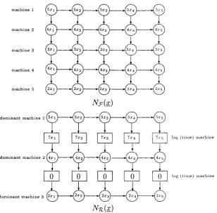
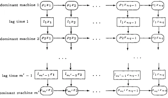
(39) CHAPTER 3. LOT STREAMING BASIC MODELS. 31. (1,1) to (m, q) in N(x); and a subpath of a critical path as a critical segment. If (i, k) — (i + 1, /c) is a critical segment for some machine i (1 < i < m — 1) then /c is a critical sublot, and if (i, A;) — (?', k + 1) is a critical segment for some sublot k (1 < k < q — 1) then i is a critical machine. They prove that in any network of optimal sublot sizes, every sublot is critical, and that there exists a vector of optimal sublot sizes x_ for which N(x) contains at least two critical machines from sublot k for 1 < k < q — 1. Based on this properties they obtain a closed form for the optimal sublots sizes for the 3 machine flow shop. Glass & Potts (1998) expand this result to environments with more machines, introducing the concept of dominant machines. They define a machine v to be dominated by machines u and w (u < v < w) if v-l. * IE* \i=u. A machine is dominant if it is not dominated by any other two machines. They prove that the machine capacity constraints of a dominated machine does not come into consideration when finding optimal sublot sizes. Glass & Potts (1998) give an O(m)-time algorithm to find the dominant machines in any m machine flow shop. After applying the algorithm to a lot streaming problem, say F, a new related problem 1Z, with m! machines, is obtained. Problem TZ consists of alternating capacitated and lag machines starting and finishing with a capacitated machine. Capacitated machine v! in 1Z (1 < v! < m!) is associated with dominant machine fiui in T with the same processing time, where 1 = //i < / v < fim> = m. Every dominant machine in T corresponds to a capacitated machine in 1Z. Every lag machine in 1Z corresponds to either one or more dominated machines in J7, (with processing time, or lag time, equal to the sum of the processing times of the dominated machines between the dominant machines) or is a dummy machine (with processing time zero; this happens when //„/+] = / v + 1). 72. is a relaxation of T since it corresponds to having the machine capacity constraint relaxed. For an optimal solution the machine capacity constraint.

(40) CHAPTER 3. LOT STREAMING BASIC MODELS. 32. of a dominated machine will not be tight. The. network representation of the original problem T is denoted by. NT(x_), and NTZ(X_) denotes the network representation for problem TZ. There is a vertex (it', k) in N-n(x) for 1 < u' < m', which corresponds to a capacitated machine vertex ( / v , k) in Nf(x_) with weight p^/Zk',. an. d a vertex [u1, k]. for every lag machine in TZ with weight luiXk where. Pi. when. /J-U'+I. 7^ AV + 1). an. d /u' = 0 when / v + i = /V + 1- There are arcs. directed from (u',k) to [u',k] and from [u'.k] to («' 4- l,k) in N-n(x), for 1 < it' < m' — 1 and 1 < fc < g, and an arc from («', A;) to (u', k + 1) for 1 < u' < m' and 1 < /c < q — 1. As an example consider the case where m = 5 and the processing times are given by p\ = 5.p2 = 4,p 3 = 3,£>4 = 4 and p 5 = 2. The corresponding network graphs for N?(x), and. N-JI(X). are. given in Figure 3.3. A block B(u, i; v,j; x_) in Np(x) is composed of all paths from vertex (it, i) to vertex (v,j), except those that have a segment on some machine other than u a n d v . T h e y a r e o f t h e f o r m ( u , i ) — ... — ( u , k) — . . . — (;;, k) — . .. — ( v , j ) .. A block is said to be a critical block if all of its segments are critical. The following theorem states the structure of an optimal solution in the network representation of a one job lot streaming problem. Theorem 3.1 There exists a vector of optimal sublot sizes x_ for the original problem T for which Njr(x_) has critical blocks 5 ( / v ; ^/v; /V+i; h^, 1 < u' < m! — 1 for some integers hi,...,. x;. x) for. hmi, where 1 = hi < h2 < ... <. hm> = q, and Xk+1 for. TH^.. +l. hui < k < hu>+i — 1 and 1 < u' < m' — 1. Finally to solve the problem they focus on the vector of integers. h = (hi,h,2, •.. ,hmi). where hi = 1 and hm> = q. Note that equation (3.5).

(41) CHAPTER 3. LOT STREAMING BASIC MODELS. 33. machine 1. machine 2. machine 3. dominant machine 1 \5xl. H5X2. 5. dominant machine 2 Uxi 1. 0 dominant machine 3 [2xl 1. »( Axo). lag (time) machine. H4i. 0. 0. H2x2. 14 2x. 0. 0. Figure 3.3: Network Nr(x),. lag (time) machine. and ArTC(x). defines a recursive relationship from which, for a fixed h, the vector of sublot sizes x_ can be calculated. That is, if we define Pu< =. then under /i, X. J. =. for hu> < j < hui+i. and so. The makespan in this case is given by K'. — 1,.

(42) CHAPTER 3. LOT STREAMING BASIC MODELS. 34. So that the makespan M(h) can be computed in O(m') time for a fixed h. There are O(qm'~2) feasible vectors h which define critical blocks so to obtain the optimal solution requires O(m + m'q"1'"2) time.. 3.4. A two-machine flow shop model. In this section we study a continuous lot streaming model set in a two machine flow shop with multiple jobs, set up times, and transportation times, F2\qj, Sij, tj\Cma,x. Vickson (1995) has analysed this model, focusing on the idle time between machines. He shows that the makespan minimisation reduces to a simple two machine flow shop without lot streaming. However he says "we do not currently posses an intuitive explanation of why the setup time, processing time and lot streaming effects collapse into such a simple form". In this section we give more insight into why this happens, using a network representation for the problem. The data for any given instance of the problem comprise • qj the number of sublots for each job j (j = 1,... n), • ptj the processing time of job j on machine i (for j = 1 , . . . n, and z = l,2), • s^ the setup time of each job j on each machine i (for j = 1,... n, and i — 1, 2), • tj sublot size dependent transportation time, and • Tj a fixed transportation time for each job j = 1 , . . . , n. The sublot size dependent transportation time portraits the fact that the transportation time may vary depending on the amount of items being transported, and the fixed transportation time represents the time taken every time a sublot of a particular job j is passed along form machine 1 to 2 in the flow shop. Interleaving of sublots (preemption) is not allowed, and the setups are anticipatory (they can start before the job arrives to the machine). If C<j(j) is the completion time of the job in the j - t h position in sequence a;.

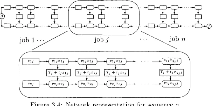
(43) CHAPTER 3. LOT STREAMING BASIC MODELS. 35. then, Ctr(n) is the completion of the last job in sequence a, and the objective is to find ff(n),. a,xkj. the sequence of jobs a (a permutation of the n jobs) and sublot sizes (1 < k < qj) for each job j = 1,.. . n that minimize the makespan of the n jobs to schedule. Any solution to this model is determined by two elements, the sublot sizes for each job, and the sequencing of jobs. We show why these two elements can be tackled separately in Theorem 3.2, give a formula for the optimal sublot sizes of each job in Theorem 3.3, and show that there is a simple rule to sequence all jobs in Theorem 3.4. Our aim is to clarify the effect the setups and transportation times have on the solution.. Tj. +. 'jz3j. Figure 3.4: Network representation for sequence a. For a given sequence of jobs a, numbered for convenience as a = ( 1 , . . . , n), we choose to represent the problem with the network shown in Figure 3.4. This network representation follows similar ideas to the network for a single job explained in Section 3.2. We have 3 X^"=i qj + 2(n+\) nodes. The circular node (5 represents the start of the schedule, while the circular node / represents the finishing of the schedule. The oval nodes represent the processing time of sublot k of job j on machine i with associated weight XkjPij. The arcs joining them horizontally represent the machine capacity constraints in-.

(44) CHAPTER 3. LOT STREAMING BASIC MODELS. 36. dicating that sublot x/t-ij must be completed on machine j before sublot x^ starts its processing (k = 2 , . . . , qj). A setup must be performed before we start processing the first sublot on the first machine which is represented by an arc is directed from the rectangular node with weight s\j to the node with weight PIJXIJ. For the same reason, the rectangular node with weight S2j, representing the setup on the second machine, precedes work on the first sublot on the second machine. The total transportation time between the first machine and the second for sublot xkj is 7} + tjXk}. This is expressed by the arcs and the rectangular node with weight T3 + tjXkj that join sublot xkj between machine one and two. The makespan of the n jobs under sequence a is the length of the longest path joining node j3 to / in the network. If the schedule starts at time 0, then the weight associated with node /3 is zero. There is a vector of sublot sizes for each job. We will use the notation xj to refer to the sublot sizes of job j . That is, x? — (.rl7-,... -xqjJ). For a specific job j and its vector of sublot sizes x-7, let M(j,xJ). = sij +. For j < n, M(j,x_j). max < ^pijXkj - ~VJ U = l. + Tj + tjXk*j + ^ P2jXkj > . k=k* ). (3.6). is the length of the longest path from the setup of job. j in the first machine to the setup of the job j' + 1 on the second machine. T h e makespan of sequence a with sublot sizes X = (xu..... denoted by Cmax(a,X),. xqi i , . . . , x\n,...,. xQnn),. can be calculated as j ' - l. + P2j), max <. max { £ (sij + pij) + M(j*,x? ) 1<7*<" j = l. (3.7) +. E. (S2j+P2j)}. That is, the longest path from node /3 to node / (see figure 3.4) goes along machine two all the way form job 1 to job n, or starts on the first machine and goes down on a particular sublot k* of a job j* to machine two and continues on machine 2 to job n, or goes along the first machine until job n in a partiuclar sublot k*. The only part in the expression for. Cnmx(a,X),. in equation (3.7), that depends on the sublot sizes of the jobs is M(j*,xJ')..

(45) CHAPTER 3. LOT STREAMING BASIC MODELS. 37. This is true regardless of the sequence a. Hence, it is always better to use the sublot sizes that minimise M(j*,x_j') for any a. This yields the following theorem. Theorem 3.2 For the F2\qj, s^, tj\Cmax model, the sublot size decision is independent of the sequencing decision. The optimal sublot sizes for job j are the ones that minimise M(j,x?) for j = 1 . . . n. To find out the size of the optimal sublot, let us focus on the value of M(j, xj>). Equation (3.6) can be rewritten as M{j,x?) = {8lj + T3 - tj) + max {]£(pij + tj)xkj + J2 fa + h)xk3}-. -. 9 j. fe=i. (3.8). k=k*. Observe that the first term s^ + Tj — tj is constant with respect to x-7. Not only that, but the second term is the expression for the makespan of an qsublot single job two-machine flow shop model with {pij + tj) processing time on the first machine, and (p2j + tj) processing time in the second machine as explained in Section 3.3 (equation 3.4). The optimal sublot sizes are given by the geometric progression of equation (3.3) derived by Potts & Baker (1989). Hence, we can state the following theorem. Theorem 3.3 The sublot sizes x? = (x\j,...,. xqj) that minimise. M(j,x>). (1 < j < n) are given, for k = 1,.. ., qj, by (P2j+tj\k-\. K. y. (. 3. .. 9. ). We now focus on the sequencing decision. Fix the sublot sizes to be the ones given by equation (3.9), which from Theorem 3.3 we know to be optimal. Note that we have reduced the problem to one without transportation times. In the reduced problem (without transportation times and sublot size decision) the setup time are s[j — s\j + 7} — t:i. and ,s'.2l — .v2?-, while the.

(46) CHAPTER 3. LOT STREAMING BASIC MODELS. 38. job processing times are p\j = pXj + tj, p'2j = jhj + tj o n machine 1 and 2 respectively. From the properties of the critical paths in a two-machine flow shop (Potts & Baker 1989), we can write p\j — a, = p'2j — bj = g3, where aj is the processing time of the first sublot on the first machine, and b3 is the processing time of last sublot on the second machine. That is o.j = p\^x\^ and bj = p'2jX*.j. The expression for the makespan of any sequence a, CmiLX(a, X), in equation (3.7), depends upon the job sequence which minimises the second term. It can be rewritten as. The last term in the above expression is independent of the job sequence. While the first term is the expression for the makespan of the n job two machine flow shop model with p\j — (s[j + aj) processing time on the first machine, and p\j = (sL + bj) processing time on the second machine. This problem is solved using a Johnson SPT(1)-LPT(2) sequence, as explained in Chapter 2. Hence we have the following theorem. Theorem 3.4 For the. F2\qj, s^-, tj\Cmax model, an optimal job order is an SPT(1)-LPT(2). sequence with respect to p\j, and p2j processing times in the. first and second machine respectively where p*j = s\j + Tj — tj + (pij + tj)x\j, P*2j = S2j + (P2j + tj)x*QjJ,. and x*kj =. We have reduced the problem to one without lot streaming, where the optimal sublot sizes are given by equation (3.9), and the jobs are ordered according to Johnson's SPT(1)-LPT(2) rule over p*^ and p*2j, as given above. W7e have shown that the sublot sizes of the jobs are not influenced by the job sequence or the setup times, and can be determined solely on the relationship between the processing times on the machines and the transportation times. On the other hand, the sequencing decision involve both the setup and transportation times as well as the relative order of the processing times of the different jobs. We have also made clear the reduction of this extended model.

No results found