Scheduling Problems with Integrable Learning and
Forgetting Effects
Peng-Jen Lai and Wen-Chiung Lee*, Member, IAENG
Abstract-Scheduling problems with learning effect have been widely studied and discussed. However, there are situations that the forgetting effect might exist as well. In this paper, we propose a model with the considerations of both effects. We then derive the optimal schedules for some single-machine scheduling problems.
Index terms- forgetting effect, learning effect, makespan, total completion time
Ⅰ. Introduction
In many realistic manufacturing situations, the marginal costs decline as firms produce more of a product or the workers gain knowledge or experience, which is known as the learning effect in the literature. For instance, Biskup [1] pointed out that the worker skills improve by processing of similar tasks repeatedly; workers are able to perform setup, to deal with machine operations or software, or to handle raw materials and components at a greater pace. He first brought the idea of learning effect into scheduling problems, and many researchers have devoted to this topic since then. For more scheduling models and problems with learning effects, the readers can refer to the extensive reviews [2-3]. Kuo and Yang [4] studied the learning effect and the deteriorating jobs on a single machine. They provided the optimal solution for the problem to minimize the sum of weighted earliness, tardiness and due-date penalties given that all jobs have a common due date. Lai and Lee [5] proposed a learning effect model in which the actual job processing time is a general function of the normal
Manuscript received Nov-21.2013. The first author was supported by the NSC of Taiwan, ROC, under NSC-102-2221-E-017-014 and the second author was supported by the NSC of Taiwan, ROC, under NSC-100-2221-E-035-029-MY3.
Peng-Jen Lai is with the Department of Mathematics, National Kaohsiung Normal University, Kaohsiung, Taiwan (email: [email protected]).
Wen-Chiung Lee is with the Department of Statistics, Feng Chia University, Taichung, Taiwan (email: [email protected]).
time of jobs already processed and its scheduled position. They pointed out that many existing models in literature are the special cases of their proposed model. In addition, they derived the optimal sequences for several single- machine problems. Rudek [6] considered the makespan problem on the flowshop environment. He discussed the computational complexity and provided the solution algorithm for the problem. Wang and Wang [7] provided the worst-case analysis for several flowshop scheduling problems when the learning effect is an exponential function. Yin and Xu [8] considered both the effects of learning and deterioration. They provided the optimal schedules for some single- machine scheduling problems. Zhu et al. [9] studied some single-machine problems with the learning effect and resource allocation in a group technology environment. They provide the optimal solutions for the problems to minimize the weighted sum of makespan and total resource cost, and the weighted sum of total completion time and total resource cost. Kuo et al. [10] tackled two unrelated parallel-machine problems with the consideration of the past-sequence- dependent setup time and learning effects. They showed that the problems to minimize the total absolute deviation of job completion times and the total load on all machines remain polynomially solvable. Zhang et al. [11] derived the optimal scheduling for some single- machine problems with sum-of- logarithm-processing-time- based and position-based learning effects. Bai et al. [12] considered the group technology on a single machine with the effects of learning and deterioration. They derived the optimal schedules for the makespan and the total completion time problems. Furthermore, Bai et al. [13] provided the optimal solutions for some single-machine problems with general exponential learning effects.
who considered both the learning and forgetting effects. They studied the total completion time problem with family setup time on a single machine. Nembhard and Uzumeri [15] pointed out that the industrial organizations are increasingly moving toward shorter product cycle times and shorter runs. Workers in this environment must constantly learn new skill, technology, and processes. Thus, forgetting effects might occur in these situations. Jabera et al. [16] also mentioned that learning and forgetting are mirror images of each other. Globerson et al. [17] and Shtub et al. [18] confirmed the finding that the power-based model is appropriate for capturing the forgetting effects. Lai and Lee [19] mentioned that the forgetting effect might exist when the study of the whole process is complicated and it takes years to learn. Thus, we propose a model with both the learning and forgetting effects in this note. We derive the optimal sequences for some single-machine problems. The remainder of this paper is organized as follows. In section 2, we describe the model. In Section 3, we provide some lemmas and prove that some single-machine problems, such as minimizing the makespan, the total completion time, the total weighted completion time, the maximum lateness, the maximum tardiness, and the total tardiness, are polynomially solvable. The conclusion is given in the final section.
II. Problem Formulation
There are n jobs to be processed on a single machine.
For each job j, there is a normal processing time pj, a
weight
w
j and a due date dj. Due to the learning andforgetting effects, the actual processing time of job j, pAj[r]
is
1 [ ] 1 1
[ ] 1 1
[ ] 1 0 0
[ ]
0 0
0 0
(1 ( , ) ), if [1 ( , )
( , ) ] , if
r
k k k
r k k k
r
k k k
r p
j
r p
A j r
j
r p
p f x r dxdr r m
p p f x r dxdr
g x r dxdr r m
(1)
if it is scheduled in the rth position in a sequence for
1, 2, ,
r n, where p[k] denote the normal processing
time of the job scheduled in the kth position in a sequence,
m is the position where the forgetting effect first occurs, and 12 n are the weights contributing to the processing time of jobs. It is assumed that
: [0, ) [0, ) (0,1]
f is integrable and non-increasing with respect to x for every fixed y , and is non-increasing with respect to y for every fixed x, and
0 0
( , ) 1
f x r dxdr
. It is also assumed that g: [0, ) [1, ) (0,1] is integrable and non-decreasing with respect to x. Furthermore, we assume that( , ) ( , )
f x r g x r (2) forx0, r0 and
1 2 1 2
( , ) ( , ) ( , ) ( , )
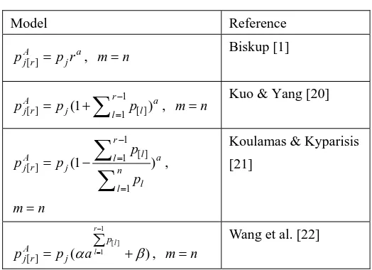
f x r f x r g x r g x r (3) for 0x1x2 0r. It is seen from Table 1 that many existing models [1, 20-22] are special cases of our proposed model. In this paper, we will use the notation Cj ,
j j
j C d
[image:2.595.297.559.421.611.2]L and Tj max{0, Cjdj} to denote the completion time, the lateness and the tardiness of job j.
Table 1. A list of the special cases (existing models) of
our model
Model Reference
[ ]
A a
j r j
p p r , mn Biskup [1]
1 [ ] (1 1 [ ])
r
A a
j r j l l
p p p
, mn Kuo & Yang [20]1 [ ] 1 [ ]
1
(1 )
r l
A l a
j r j n
l l
p
p p
p
,n
m
Koulamas & Kyparisis [21]
1 [ ] 1
[ ] ( )
r l l
p A
j r j
p p a
, mnWang et al. [22]
III. Single-machine problems
First, we derive some lemmas to be used in the proofs of the properties
Lemma 1: (1)[ ( ,f x y1)g x y( , 1)][ (f xt y, 2)
2 2 2
( , )] ( , ) ( , ) 0
g xt y f x t y g x t y for
1
, 0, t0 and y1y2.
Proof. Let G( ) (1)[ ( ,f x y1)g x y( , 1)]
2 2
[ (f x t y, ) g x( t y, )]
2 2
( , ) ( , )
f x t y g x t y
Taking the derivative of G( ) , we have from Equation (3) that
2 2
'( ) [ x( , ) x( , )]
G t f xt y g xt y
2 2
[ x( , ) x( , )]
t f x t y g x t y
2 2 2
= [t fx(xt y, ) fx(xt y, )gx(xt y, )
2
( , )] 0
x
g x t y
In addition, let
1 1 2 2
( ) ( 1)[ ( , ) ( , )] [ ( , ) ( , )]
h f x y g x y f x y g x y
2 2
( , ) ( , )
f x y g x y
.
From Equation (2), we have
1 1 2 2
'( ) ( , ) ( , ) ( , ) ( , ) 0
h f x y g x y f x y g x y . With the condition that h(1)0, we have h( ) 0 for
1
. Since G(0)h( ) 0 and G'( ) 0, it follows that G( ) 0. This completes the proof of Lemma 1.
Lemma 2(1)[ ( ,f x y1)g x y( , 1)][ (f x t ,y2) 2
( , )]
g x t y
[ (f xt y, 2)g x( t y, 2)]0
for 1, 0, t0, 0 1 and y1y2.
Proof:LetH( ) (1)[ ( ,f x y1)g x y( , 1)][ (f x t ,y2)
2
( , )]
g x t y
[ (f xt y, 2)g x( t y, 2)]. Taking the first derivative of H( ) , we have from Equation (3) and 1 that
1 1 2
'( ) ( , ) ( , ) [ x( , )
H f x y g x y t f x t y
2
( , )]
x
g x t y
[ (f xt y, 2)g x( t y, 2)]
1 1 2 2
( , ) ( , ) [ x( , ) x( , )]
f x y g x y t f x t y g x t y
[ (f xt y, 2)g x( t y, 2)].
Let G( , ) f x y( , 1)g x y( , 1)t f[ x(xt y, 2) 2
( , )]
x
g x t y
2 2
[ (f x t y, ) g x( t y, )]
.
It is seen from Equation (3) that G( , ) is non-increasing with respect to and . Furthermore,
let
1 1 2 2
( ) ( , ) ( , ) [ x( , ) x( , )]
h t f x y g x y t f xt y g xt y
2 2
[ (f x t y, ) g x( t y, )]
.
Taking the derivative of h t( ), we have from Equation (3) that
2
2 2 2
'( ) [ x( , ) x( , )] [ xx( , )
h t f xt y g xt y t f xt y
gxx(xt y, 2)][fx(xt y, 2)gx(xt y, 2)]
2
2 2
[ xx( , ) xx( , )] 0
t f x t y g x t y
From Equation (2), we have
1 1 2 2
(0) ( , ) ( , ) [ ( , ) ( , )] 0
h f x y g x y f x y g x y . It implies that G(1,1)h t( )0. Since G( , ) is non- increasing with respect to and , we have
( , ) 0
G . It implies that H( ) is non-decreasing with
respect to . Therefore, H( ) H(1)0. This completes the proof of Lemma 2.
Lemma 3: (1) ( ,f x y1) f x( t ,y2)
2 2
[ (f x t y, ) g x( t y, )]
g x( t ,y2)0 for
1
, 0, t0 and y1y2.
Lemma 4: (1) ( ,f x y1)f x( t ,y2) 2
( , )
g x t y
[ (f xt y, 2)g x( t y, 2)]0
for 1, 0, t0, 0 1, and y1y2.
Lemma 5: (1) ( ,f x y1)f x( t y, 2) 2
( , ) 0
f x t y
for 1 , 0 , t0 and
1 2
y y .
Lemma 6: (1) ( ,f x y1)f x( t ,y2)
2
( , ) 0
f x t y
for 1, 0, t0, y1y2, and 0 1.
The proofs of Lemmas 3-6 are similar to those of Lemmas 1 and 2, and thus omitted.
Next, we will prove the following properties using the pairwise interchange technique. Suppose that
1 ( , , , )
S j i and S2 ( , , , i j ), where and each denote a partial sequence. Furthermore, we assume that there are r-1 scheduled jobs in . In addition, let A denote the completion time of the last job in . The completion times of jobs j and i in S1 are
1
[ ] 1
1 1 1
[ ] [ ]
1 1
( , ) if
( )
( , ) ( , ) if
r
j k k
k
j r r
j k k j k k
k k
A p f p r r m
C S
A p f p r p g p r r m
(4)and 1 [ ] 1 1 1 [ ] 1 1 [ ] 1 1 [ ] 1 1 [ ] 1 1 [ ] [ 1 ( , )
( ) if
( , 1 ) ( , )
[ ( , 1) if + ( , 1)]
[ ( , ) (
r j k k
k
i r
i k k r j k
r j k k
k r
i k k r j k
r
k k r j k
r
j k k k k k
A p f p r
C S r m
p f p p r
A p f p r
p f p p r r m
g p p r
A p f p r g p
1 ] 1 1 [ ] 1 1 [ ] 1 , )] [ ( , 1) if + ( , 1)]r k r
i k k r j k
r
k k r j k
r
p f p p r r m
g p p r
Similarly, the completion times of jobs i and j in
S
2 are1
[ ] 1
2 1 1
[ ] [ ]
1 1
( , ) if
( )
[ ( , ) ( , )] if
r
i k k
k
i r r
i k k k k
k k
A p f p r r m
C S
A p f p r g p r r m
(6)and
1 [ ] 1
2 1
[ ] 1 1
[ ] 1
1 [ ] 1 1
[ ] 1
1
[ ] [ ] 1
( , )
( ) if
( , 1 ) ( , )
[ ( , 1) if + ( , 1)]
[ ( , ) ( ,
r i k k
k
j r
j k k r i k
r i k k
k r
j k k r i k
r
k k r i k
r
i k k k k k
A p f p r
C S r m
p f p p r
A p f p r
p f p p r r m
g p p r
A p f p r g p
11 1
[ ] 1 1
[ ] 1
)] [ ( , 1) if ( , 1)]
r k r
j k k r i k
r
k k r i k
r
p f p p r r m
g p p r
(7)
Property 1. The optimal schedule for the makespan
problem is obtained by the shortest processing time (SPT) rule.
Proof. We prove the property by contradiction. Consider an
optimal schedule S1 where the jobs do not follow the SPT
rule. In this schedule, there are at least two adjacent jobs,
say job j followed by job i, such that pj pi. We now
perform an adjacent pairwise interchange of jobs i and j, leaving all the other jobs in their original positions, to derive a new sequence S2. Taking the difference between Equations (5) and (7), we have
1 2
( ) ( )
i j
C S C S
Substituting 1
[ ] 1
r k k k
x p
, pj/pi, t pi, r,1
y r and y2 r 1 into Equation (8), we have from Lemmas 1, 3 and 5 that C Si( 1)C Sj( 2). This contradicts the optimality of S1 and proves that the jobs must be
scheduled according to SPT rule in the optimal sequence.
Property 2. The optimal schedule for the total completion
time problem is obtained by the SPT rule.
Proof. The proof is omitted since it is similar to that of
Property 1.
We show in the next property that the WSPT rule provides an optimal solution for the total weighted completion time problem if the processing times and the
weights are agreeable, i.e., pi pj implies wiwj for
all jobs i and j.
Property 3. The optimal schedule for the total weighted
completion time problem is obtained by the WSPT rule if the processing times and the weights are agreeable.
Proof. We prove the property by contradiction. Consider an
optimal schedule S1 where the jobs do not follow the
WSPT rule. In this schedule, there are at least two adjacent
now perform an adjacent pairwise interchange of jobs i and
j, leaving all the other jobs in their original positions, to
derive a new sequence
S
2. From Equations (4)-(7), wehave that[w C Sj j( 1)w C Si i( 1)] [ w C Si i( 2)w C Sj j( 2)]
1 1
[ ] [ ]
1 1
1 [ ] 1 1
[ ] 1
( , )( )( ) ( , 1) ( , 1 ) if ( , )( )( )
r r
k k i j j i i i k k r j
k k
r
j j k k r i k
r
k k i j j i k
i i
f p r w w p p wp f p p r
w p f p p r r m
f p r w w p p
wp
1 1
[ ] [ ]
1 1
1 1
[ ] [ ]
1 1
1 1
[ ] [ ]
1 1
[ ( , 1) ( , 1)]
[ ( , 1) ( , 1 ) ] if . (9) [ ( , ) ( , )]( )(
r r
k k r j k k r j
k k
r r
j j k k r i k k r i
k k
r r
k k k k i j j k k
f p p r g p p r
w p f p p r g p p r r m
f p r g p r w w p
1 1
[ ] [ ]
1 1
1 1
[ ] [ ]
1 1
)
[ ( , 1) ( , 1)] [ ( , 1)+ ( , 1 ) ] if
i
r r
i i k k r j k k r j
k k
r r
j j k k r i k k r i
k k
p
wp f p p r g p p r
w p f p p r g p p r r m
Substituting 1
[ ] 1
r r k k
x p
, pj/ pi, t pi, r,/ ( )
j i j
w w w
, wi/ (wiwj) , y1r , and
2 1
y r into Equation (9), we have from Lemmas 2, 4
and 6 that w C Sj j( 1)w C Si i( 1)w C Si i( 2)w C Sj j( 2) . This contradicts the optimality of S1 and proves that the
jobs must be scheduled according to WSPT rule in the optimal sequence.
Property 4. The optimal schedule for the maximum
lateness problem is obtained by the EDD rule if the processing times and the due dates are agreeable.
Property 5. The optimal schedule for the maximum
tardiness problem is obtained by the EDD rule if the processing times and the due dates are agreeable.
Property 6. The optimal schedule for the total tardiness
problem is obtained by the EDD rule if the processing times and the due dates are agreeable.
IV. Conclusions
In this paper, we consider a learning-and-forgetting-effect model. We first show many existing models in the literature are special cases of our proposed model. We then derive the
optimal schedules for some single-machine problems, which includes the makespan, the total completion time, the total weighted completion time, the maximum lateness, the maximum tardiness. Considering other models with learning and forgetting effects might be interesting.
References
[1] D. Biskup, Single-machine scheduling with learning considerations,
European Journal of Operational Research 115 (1999) 173-178.
[2] D. Biskup, A state-of-the-art review on scheduling with learning effect,
European Journal of Operational Research 188 (2008) 315-329.
[3] A. Janiak, R. Rudek, Experience based approach to scheduling
problems with the learning effect, IEEE Transactions on Systems,
Man, and Cybernetics - Part A 39 (2009) 344-357.
[4] W.H. Kuo, D.L. Yang, A note on due-date assignment and single-
machine scheduling with deteriorating jobs and learning effects,
Journal of the Operational Research Society 62 (2011) 206-210.
[5] P.J. Lai, W.C. Lee, Single-machine scheduling with general sum-of-
processing-time-based and position-based learning effects,
OMEGA-The International Journal of Management Science 39
(2011) 467-471.
[6] R. Rudek, Computational complexity and solution algorithms for
flowshop scheduling problems with the learning effect, Computers &
Industrial Engineering 61 (2011) 20–31.
[7] J.B. Wang, M.Z. Wang, Worst-case analysis for flow shop scheduling
problems with an exponential learning effect, Journal of the
Operational Research Society 63 (2012) 130-137.
[8] Y.Q. Yin, D.H. Xu, Some single-machine scheduling problems with
general effects of learning and deterioration, Computers and
Mathematics with Applications 61 (2011) 100–108.
[9] Z.G. Zhu, L.Y. Sun, F. Chu, M. Liu, Single-machine group scheduling
with resource allocation and learning effect, Computers & Industrial
Engineering 60 (2011) 148–157.
[10] W.H. Kuo, C.J. Hsu, D.L. Yang, Some unrelated parallel machine
scheduling problems with past-sequence-dependent setup time and
learning effects, Computers & Industrial Engineering 61 (2011)
179–183.
[11] X.G. Zhang, G.L. Yan, W.Z. Huang, G.C. Tang, A note on machine
scheduling with sum-of-logarithm-processing-time-based and
position-based learning effects, Information Sciences 187, (2012)
298–304.
[12] J. Bai, Z.R. Li, X. Huang, Single-machine group scheduling with
general deterioration and learning effects, Applied Mathematical
Modelling 36 (2012) 1267-1274.
general exponential learning effect, Applied Mathematical
Modelling 36 (2012) 829–835.
[14] W.H. Yang, S. Chand, Learning and forgetting effects on a group
scheduling problem, European Journal of Operational Research 187
(2008) 1033–1044.
[15] D.A. Nembhard, M.V. Uzumeri, Experiential learning and forgetting
for manual and cognitive tasks, International Journal of Industrial
Ergonomics 25 (2000) 315-326.
[16] M.Y. Jabera, H.V. Kherb, D.J. Davis, Countering forgetting through
training and deployment, International Journal of Production
Economics 85 (2003) 33–46.
[17] S. Globerson, N. Levin, A. Shtub, The impact of breaks on forgetting
when performing a repetitive task, IIE Transactions 21 (1989)
376–381.
[18] A. Shtub, N. Levin, S. Globerson, Learning and forgetting industrial
skills: experimental model, International Journal of Human Factors
in Manufacturing 3 (1993) 293–305.
[19] P.J. Lai, W.C. Lee, Single-machine scheduling with learning and
forgetting effects, Applied Mathematical Modelling 37 (2013)
4509-4516.
[20] W.H. Kuo, D.L. Yang, Minimizing the total completion time in a
single-machine scheduling problem with a time-dependent learning
effect, European Journal of Operational Research 174 (2006)
1184-1190.
[21] C. Koulamas, G.J. Kyparisis, Single-machine and two-machine
flowshop scheduling with general learning function, European
Journal of Operational Research 178 (2007) 402-407.
[22] J.B. Wang, D. Wang, L.Y. Wang, L. Lin, N. Yin, W.W. Wang, Single
machine scheduling with exponential time-dependent learning effect
and past-sequence- dependent setup times, Computers and