On the Capability of a Fuzzy Inference System with Improved Interpretability

(1)

On the Capability of a Fuzzy Inference System

with Improved Interpretability

Hirofumi Miyajima

†1

, Noritaka Shigei

†2

, and Hiromi Miyajima

†3

Abstract—Many studies on modeling of fuzzy inference systems have been made. The issue of these studies is to construct automatically fuzzy systems with interpretability and accuracy from learning data based on meta-heuristic methods. Since accuracy and interpretability are contradicting issues, there are some disadvantages for self-tuning method. Obvious drawbacks of the method are lack of interpretability and getting stuck in a shallow local minimum. Therefore, the conventional learning methods with multi-objective fuzzy modeling and fuzzy modeling with constrained parameters of the ranges have become popular. However, there are little studies on effective learning methods of fuzzy inference systems dealing with interpretability and accuracy. In this paper, we will propose a fuzzy inference system with interpretability. Firstly, it is proved that the proposed model is an universal approximator of continuous functions. Further, the capability of the proposed model learned by the steepest descend method is compared with the conventional models using function approximation problems. Lastly, the proposed model is applied to obstacle avoidance and the capability of interpretability is shown.

Index Terms—fuzzy set, fuzzy inference, interpretability, universal approximator, obstacle avoidance.

I. INTRODUCTION

F

UZZY inference systems are widely used in system modeling for the fields of classification, regression, decision support system and control [1], [2]. Therefore, many studies on modeling of fuzzy inference systems have been made. The issue of these studies is to construct automatically fuzzy systems with interpretability and accuracy from learn-ing data based on meta-heuristic methods [4], [5], [9], [12], [14]. Since accuracy and interpretability are contradicting issues, there are some disadvantages for self-tuning method. Obvious drawbacks of the method are lack of interpretability and getting stuck in a shallow local minimum [6]. As the meta-heuristic methods, some novel methods have been de-veloped which 1) use GA and PSO to determine the structure of the fuzzy model [6], [7], 2) use generalized objective functions [8], 3) use fuzzy inference systems composed of small number of input rule modules, such as SIRMs and DIRMs methods [10], [11], 4) use a self-organization or a vector quantization technique to determine the initial assignment and 5) use combined methods of them [5], [14]. Since accuracy and interpretability are conflicting goals, the conventional learning methods with multi-objective fuzzy modeling and fuzzy modeling with constrained parameters of the ranges have become popular. However, there are little studies on effective learning methods of fuzzy inference

Affiliation: Graduate School of Science and Engineering, Kagoshima University, 1-21-40 Korimoto, Kagoshima 890-0065, Japan

corresponding auther to provide email: [email protected] †1email: [email protected]

†2email: [email protected] †3email: [email protected]

Ͳ ܽ௜௝ ܯ௜௝

ܿ௜௝ ܾ௜௝

[image:1.595.359.498.173.270.2]

ݔ௝

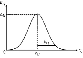
Fig. 1. The Gaussian membership function

systems dealing with interpretability and accuracy. On the other hand, fuzzy modeling with preserving interpretability is proposed by Shi [15]. However, there are no studies on the detailed capability of this type of model.

In this paper, we will propose a fuzzy inference system with interpretability. Firstly, it is proved that the proposed model is a universal approximator of continuous functions. Further, the capability of the proposed model learned by the steepest descend method is compared with the conventional models using function approximation problems. Lastly, the proposed model is applied to obstacle avoidance and the capability of interpretability is shown.

II. PRELIMINARIES

A. The conventional fuzzy inference model

The conventional fuzzy inference model is described [1].

LetZj={1,· · · , j}for the positive integerj. LetRbe the

set of real numbers. Letx= (x1,· · ·, xm) andyr be input

and output data, respectively, wherexj∈R for j∈Zm and

yr_∈_R_{. Then the rule of fuzzy inference model is expressed} as

Ri : if x1 isMi1 and · · · andxmis Mim

theny isfi(x1,· · ·, xm) (1)

, where i ∈ Zn is a rule number, j ∈ Zm is a variable number, Mij is a membership function of the antecedent part, and fi(x1,· · ·, xm) is the function of the consequent

part.

A membership value of the antecedent part µj for input

xis expressed as

µi= m ∏

j=1

Mij(xj). (2)

If Gaussian membership function is used, then Mij is expressed as follow (See Fig.1):

Mij=aijexp (

−1

2 (

xj−cij

bij )2)

(2)

, whereaij,cij andbij are the amplitude, the center and the width values ofMij, respectively.

The output y∗ of fuzzy inference is calculated by the following equation:

y∗= ∑n

i=1µi·fi

∑n i=1µi

. (4)

Specifically, simplified fuzzy inference model is known as one with fi(x1,· · ·, xm) =wi for i∈Zn, where wi∈R is a real number. The simplified fuzzy inference model is called Model 1.

B. Learning algorithm for the conventional model

In order to construct the effective model, the conven-tional learning method is introduced. The objective function

E is defined to evaluate the inference error between the desirable output yr _{and the inference output} _y∗_{. In this} section, we describe the conventional learning algorithm. Let

D={(xp₁,· · ·, xp

m, yrp)|p∈ZP}be the set of learning data. The objective of learning is to minimize the following mean square error(MSE):

E= 1

P

P ∑

p=1

(y∗_p−yr_p)2. (5)

In order to minimize the objective functionE, the param-etersα∈ {aij, cij, bij, wi}are updated based on the descent method as follows [1]:

α(t+ 1) =α(t)−Kα

∂E

∂α (6)

where t is iteration time and Kα is a constant. When Gaussian membership function with aij = 1for i∈Zn and

j∈Zm are used, the following relation holds [6].

∂E ∂cij

= ∑nµj i=1µi

·(y∗−yr)·(wi−y∗)·

xj−cij

b2

ij (7)

∂E ∂bij

= ∑nµi i=1µi

·(y∗−yr)·(wi−y∗)·

(xj−cij)2

b3

ij (8)

∂E ∂wi

= ∑nµi i=1µi

·(y∗−yr) (9)

Then, the conventional learning algorithm is shown as below [1], [2], [6].

Learning Algorithm A

Step A1 : The threshold θ of inference error and the maximum number of learning time Tmax are given. The initial assignment of fuzzy rules is to equally intervals. Let

n be the number of rules andn=dm _{for an integer}_d_{. Let}

t= 1.

Step A2 : The parameters bij, cij and wi are set to the initial values.

Step A3 : Letp= 1.

Step A4 : A data(xp₁,· · ·, xp

m, ypr)∈D is given.

Step A5 : From Eqs.(2) and (4), µi andy∗ are computed.

Step A6 : Parameterscij,bijandwiare updated by Eqs.(7), (8) and (9).

Step A7: Ifp=P then go to Step A8 and ifp < P then go to Step A3 withp←p+ 1.

Step A8: Let E(t) be inference error at step t calculated by Eq.(5). IfE(t)> θ and t < Tmax then go to Step A2 witht←t+ 1else ifE(t)≤θandt≤Tmaxthen the algorithm terminates.

Step A9: If t > Tmax and E(t)> θ then go to Step A3 withn=dm _as_d_←_d_{+ 1} _and_t_{= 1.}

C. The proposed model

It is known that Model 1 is effective, because all the parameters are adjusted by learning. On the other hand, all the parameters move freely, so interpretability capability is low. Therefore, we propose the following model.

Ri1···im _{: if} _x

1 isMi11 and · · · and xm isMimm

theny isfi1···im(x1,· · ·, xm) (10)

, where1≤ij≤lj,j∈Zm.

µi1···im=

m ∏

j=1

Mijj(xj) =Mi11(x1)·· · ··Mimm(xm) (11)

y= ∑

i1· · ·

∑

imµi1···imfi1···im(x1,· · ·, xm)

∑ i1· · ·

∑

imµi1···im

(12)

In this case, the model with fi1,···,im(x1· · ·, xm) = wi1,···,im and triangular membership function has already

proposed in the Ref. [15].

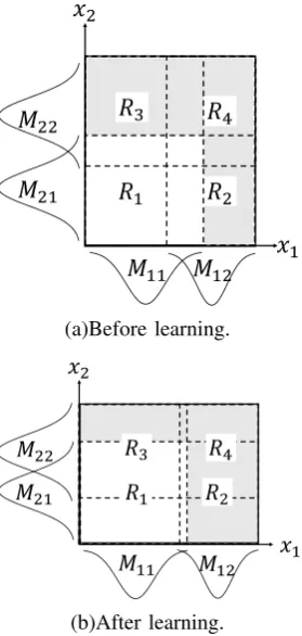
We will consider a model with fi1,···,im(x1,· · ·, xm) = wi1,···,im and Gaussian membership functions. The model is

called Model 2(See Fig.2). Remark that Model 2 is one that the parameters of membership function for each variable are adjusted by learning.

Learning equation for Model 2 is obtained as follows:

∂E ∂Mijj

=∑

i1

· · ·∑

ij−1

∑

ij+1

· · ·∑

im µi1···im

∑ i1· · ·

∑

imµi1···im

·(y∗−yr)·(y∗−wi1···im)

(13)

∂E ∂wi1···im

= ∑ µi1···im

i1· · ·

∑

imµi1···im

·(y∗−yr) (14)

When Eq.(15) is used as a membership function, the following equations foraijj,cijj andbijj are obtained;

Mijj(xj) =aijjexp

 ₋1

2 m ∑

j=1

(xj−cijj) 2

b2

ijj



 (15)

∂Mijj ∂aijj

= exp  ₋1

2 m ∑

j=1

(xj−cijj) 2

b2

ijj



 (16)

∂Mijj ∂cijj

= (xj−cijj) b2

ijj

exp  ₋1

2 m ∑

j=1

(xj−cijj) 2

b2

ijj

  (17)

∂Mijj ∂bijj

= (xj−cijj) 2

b3

ijj

exp  ₋1

2 m ∑

j=1

(xj−cijj) 2

b2

ijj

(3)

[image:3.595.101.241.52.346.2]

ଵଵ ଵ ଶ ଵଶ ଶଵ ଶଶ ଵ ଶ ଷ ସ (a)Before learning. ଵ ଶ ଵଵ ଵଶ ଶଵ ଶଶ ଵ ଶ ଷ ସ (b)After learning.

Fig. 2. The figure to explain Model 2 withm= 2andi1=i2= 2. The assignment (a) of fuzzy rules for Model 2 is transformed into the assignment (b) after learning.

Mamdani type model is special case of Model 2 [7]. It is the model with the fixed parameters of antecedent part of fuzzy rule and membership function assigned to equally intervals [12], [14]. The model is called Model 3. It has good interpretable capability , but the accuracy capability is law. Therefore, TSK model with the weight of linear functionfi(x1,· · ·, xm)is introduced as a generalized model

of Model 3 [3]. The model is called Model 4.

III. FUZZY INFERENCE SYSTEM ASUNIVERSAL APPROXIMATOR

In this section, the universal approximation capabilities of Model 1, 2, 3 and 4 are discussed using the well-known Stone-Weierstrass Theorem. See Ref. [2] about the mathematical terms.

[Stone-Weierstrass Theorem] [2]

Let S be a compact set with m dimensions, and C(S) be a set of all continuous real-valued functions on S. Let Ω be the set of continuous real-valued functions satisfying the conditions:

(i) Identity function : The constant functionf(x) = 1 is in Ω.

(ii) Separability : For any two pointsx1,x2∈S andx1̸=x2,

there exists af∈Ωsuch thatf(x1)̸=f(x2).

(iii) Algebraic closure : For any f, g∈Ω and α, β∈R, the functionf·g andαf+βg are inΩ.

Then, Ωis dense inC(S). In other words, for anyε >0 and any function g∈C(S) , there is a function f∈Ω such that

|g(x)−f(x)|< ε

for allx∈S.□

It means that the setΩsatisfying the above conditions can approximate any continuous function with any accuracy. Since the sets of RBF and Model 1 are satisfied with the conditions of Stone-Weierstrass Theorem, they hold for universal approximation capabilities [2], [16]. Further, we can show the result about Model 2 in the following. [Theorem]

Let Φ be the set of all functions that can be computed by Model 2 on a compact setS∈Rmas follows:

Let

Φl₁_···lm = { f(x) =

∑ i1· · ·

∑ im

∏

jMijj(xj)wi1···im

∑ i1· · ·

∑

imMijj(xj) , wi1···wm, aijj, cijj, bijj∈R,x∈S}

forMijj(xj) =aijjexp

(

−1

2

(_x

j−cij j

b_{ij j} )2)

and

Φ =

∞

∪

l1=1

· · · ∞

∪

lm=1

Φl1···lm (19)

ThenΦis dense inC(S). [Outline of Proof]

Letf andg be two functions inΦand be represented as

f(x) = ∑

i1· · ·

∑ im

∏ jM

f ijj(xj)w

f i1···im

∑ i1· · ·

∑ im

∏ jM

f ijj(xj)

(20)

g(x) = ∑

l1· · ·

∑ lm

∏ jM

g ljj(xj)w

g l1···lm

∑ l1· · ·

∑ lm

∏ jM

g ljj(xj)

(21)

for

M_if

jj(xj) =a

f ijjexp

 ₋1

2 (

xj−c f ijj bf_i

jj

)2

 (22)

M_lg

jj(xj) =a

g ljjexp

 ₋1

2 (

xj−c g ljj bg_l

jj

)2

 (23)

Then, we will show onlyαf+βg∈Φandf·g∈Φ. We define

M_if g

jljj(xj) = M

f

ijj(xj)·M

g lj(xj)

= af g_i jljjexp

 ₋1

2 (

xj−c f g ijljj bf g_i

jljj

)2

(24)

w_if g1

1···iml1···lm = w

f

i1···im+w

g

l1···lm (25) w_if g2

1···iml1···lm = w

f i1···im·w

g

l1·lm (26)

, whereaf g_i jljj, c

f g ijljj, b

f g ijljj, w

f g1

i1···wiml1···lm, w

f g2

i1···iml1···lm∈R.

By using these values,

αf+βg

= ∑

i1· · ·

∑ im

∑ l1· · ·

∑ lm

∏ jM

f g ijljj(xj)w

f g1

i1···iml1···lm

∑ i1· · ·

∑ im

∑ l1· · ·

∑ lm

∏ jM

f g ijljj(xj)

(27)

f·g

= ∑

i1· · ·

∑ im

∑ l1· · ·

∑ lm

∏ jM

f g ijljj(xj)w

f g2

i1···iml1···lm

∑ i1· · ·

∑ im

∑ l1· · ·

∑ lm

∏ jM

f g ijljj(xj)

(4)

TABLE I

INITIAL CONDITION FOR SIMULATION OF FUNCTION APPROXIMATION.

Model 1 Model 2 Model 3 Model 4

Tmax 50000 50000 50000 50000

Kc 0.01 0.01 0.0 0.0

Kb 0.01 0.01 0.0 0.0

Kw 0.1

d 3 7 4 6

Initialcij equal intervals Initialbij ₂₍_d1₋₁₎×(the domain of input) Initialwij random on[0,1]

[image:4.595.48.293.498.602.2] [image:4.595.338.512.635.751.2]

Further, Eqs.(27) and (28) have the same form as Model 2. Therefore,(αf+βg)andf·g∈Φhold.□

[Remarks]

Remark that the results using Stone-Weierstrass Theorem hold only for Model 1 and 2 with fi(x1· · ·xm) = wi and Gaussian membership function. On the other hand, Stone-Weierstrass Theorem does not always hold for Model 3, 4 and the models with triangular membership function, because the multiplicative condition fails. Further, it is an existence theorem and there is another problem whether we can get the system with high accuracy. Therefore, we need effective learning algorithm. Learning Algorithm A is a learning algorithm based on the steepest descend method.

IV. NUMERICAL SIMULATIONS

In this section, two kinds of simulations are performed to compare with the capabilities of models for learning method based on steepest descend method. In the simulations, let

aij = 1andaijj= 1 fori∈Zn andj∈Zm.

A. Function approximation

This simulation uses four systems specified by the follow-ing functions with[0,1]×[0,1].

y = sin(πx3₁)·x2 (29)

y = sin(2πx

3

1)·cos(πx2) + 1

2 (30)

y = 1.9(1.35 +e

x1_sin(13(_x

1−0.6)2)·e−x2sin(7x2))

7

(31)

y = sin(10(x1−0.5)

2_{+ 10(}_x

2−0.5)2) + 1.0

2 (32)

The condition of the simulation is shown in Table I. The value θ is 1.0×10−5 _{and the numbers of learning and test}

data selected randomly are 200 and 2500, respectively. Table II shows the results on comparison among four models. In Table II, Mean Square Error(MSE) of learning(×10−4_{) and}

MSE of test(×10−4_{) are shown. The result of simulation is}

the average value from ten trials. Table II shows that Model 1 and 2 have almost the same capability in this simulation, where♯parameter means the number of parameters.

B. Obstacle avoidance and arriving at designated point

In order to show interpretability, let us perform simulation of control problem for Model 1 and Model 2 [11]. As shown in Fig.3, the distance r1 and the angle θ1 between mobile

object and obstacle and the distance r2 and the angle θ2

TABLE II

RESULTS FOR SIMULATION OF FUNCTION APPROXIMATION.

Eq.(29) Eq.(30) Eq.(31) Eq.(32)

Model 1 learning 0.10 0.44 2.25 0.30

test 0.30 2.16 3.84 0.88

♯parameter 45 45 45 45

Model 2 learning 0.10 1.47 0.10 0.42

test 0.93 5.46 0.39 2.03

Model 3 learning 1.10 13.33 1.32 4.83

test 4.50 50.29 4.40 29.23

Model 4 learning 0.21 2.52 0.71 2.87

test 0.98 9.68 1.95 10.97

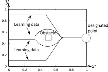
Fig. 3. Simulation on obstacle avoidance and arriving at the designated point.

between mobile object and the designated place are selected as input variables, whereθ1 andθ2 are normalized.

The problem is to construct fuzzy inference system that mobile object avoids obstacle and arrives at the designated point. From (operation) data, fuzzy inference rules for Model 1 and Model 2 are constructed from learning for data of 400 points shown in Fig. 4. An obstacle is placed at (0.5,0.5) and a designated point is placed at (1.0,0.5). The number of rules for each model is 81 and the number of attributes is 3. Then, the numbers of parameters for Model 1 and 2 are 729 and 93, respectively. The mobile object moves with the vectorAat each step, whereAxofAis constant andAy of

Ais output variable. Learning for two models are successful and the following tests are performed.

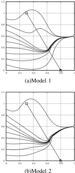
(1)Test 1 is simulation for obstacle avoidance and ar-riving at the designated place when the mobile object stars from various places (See Fig.5). Fig.5 shows the results of moves of mobile object for starting places at (0.1,0),(0.2,0),· · ·,(0.8,0),(0.9,0) after learning. As shown in Fig.5, the test simulations are successful for both

0 0.2 0.4 0.6 0.8 1

Learning data

Learning data Obstacle

designated point

(5)

TABLE III

INITIAL CONDITION FOR SIMULATION OF OBSTACLE AVOIDANCE.

Model 1 Model 2

Tmax 50000 50000

Kc 0.001 0.001

Kb 0.001 0.001

Kw 0.01

d 3 3

Initialcij equal intervals Initialbij ₂₍_d1₋₁₎×(the domain of input)

Initialwij 0.0

0 0.2 0.4 0.6 0.8 1

(a)Model 1

0 0.2 0.4 0.6 0.8 1

[image:5.595.73.255.56.480.2]

(b)Model 2

Fig. 5. Simulation for obstacle avoidance and arriving at the designated place starting from various places after learning.

models.

(2)Test 2 is simulation for the case where the mobile object avoids obstacle placed at different place and arrives at the different designated place. Simulations with obstacle placed at the place (0.4,0.4) and arriving at the designated place (1,0.6) are performed for two models. The results are successful as shown in Fig.6.

(3)Test 3 is simulation for the case where obstacle moves with the fixed speed. Simulations with obstacle moving with the speed(0.01,0.02)from the place(0.3,1.0) to the place (0.8,0.0) and arriving at the place (1,0.6) are performed. The results are successful as shown in Fig.7.

(4)Test 4 is simulation for the case where obstacle moves randomly as shown in Fig.8, where|B|is constant, and the angle θb is determined randomly at each step. Simulations with obstacle moving from the point(0.5,1.0)are perfurmed for two models. The results are successful as shown in Fig.9.

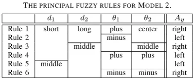
Lastly, let us consider interpretability for the proposed model. From fuzzy rules constructed for Model 2 by learning, we can find interpretable rules. Assume that three attributes

0 0.2 0.4 0.6 0.8 1

(a)Model 1

-0.2 0 0.2 0.4 0.6 0.8 1

0 0.2 0.4 0.6 0.8 1 (b)Model 2

Fig. 6. Simulation for obstacle placed at the different position(0.4,0.4)

and arriving at the different place(1.0,0.6).

0 0.2 0.4 0.6 0.8 1 1.2

0 0.2 0.4 0.6 0.8 1 (a)Model 1

0 0.2 0.4 0.6 0.8 1 1.2

0 0.2 0.4 0.6 0.8 1 (b)Model 2

[image:5.595.361.490.441.737.2]

(6)

[image:6.595.102.240.52.173.2]

Fig. 8. The obstacle moves with the vectorB, where|B|is constant and

θbis selected randomly.

-0.2 0 0.2 0.4 0.6 0.8 1 1.2

0 0.2 0.4 0.6 0.8 1

(a)Model 1

0 0.2 0.4 0.6 0.8 1 1.2

[image:6.595.106.234.233.535.2]

0 0.2 0.4 0.6 0.8 1 (b)Model 2

Fig. 9. Simulation for moving obstacle randomly and the different designated place(1.0,0.6).

are short, middle and long ford1 andd2, minus, central and

plus forθ1andθ2 and left, center and right for the direction

ofAy, respectively. Then, the principal fuzzy rules for Model 2 are constructed as shown in TableIV. They are similar to human activity to solve the problem. On the other hand, fuzzy rules for Model 1 are not so clear.

TABLE IV

THE PRINCIPAL FUZZY RULES FORMODEL2.

d1 d2 θ1 θ2 Ay

Rule 1 short long plus center right

Rule 2 minus left

Rule 3 middle middle right

Rule 4 plus plus left

Rule 5 middle left

Rule 6 minus minus right

V. CONCLUSION

In this paper, a theoretical result and some numerical simulations including obstacle avoidance are presented in order to compare the proposed model with the conventional models. It is shown that Model 1 and Model 2 with Gaussian membership function andfi(x1,· · ·, xm) =wi are satisfied with the conditions of Stone-Weierstrass Theorem, so both models are universal approximators of continuous functions. Further, in order to compare the capability of learning algo-rithms for models, numerical simulation of function approx-imation is performed. Lastly, some simulations on obstacle avoidance are performed. In the simulations, it is shown that both models are successful in all trials. Specifically it is shown that Model 2 with the small number of parameters and interpretability is constructed.

In future work, we will find an effective learning method for Model 2.

REFERENCES

[1] C. Lin and C. Lee, Neural Fuzzy Systems, Prentice Hall, PTR, 1996. [2] M.M. Gupta, L. Jin and N. Homma, Static and Dynamic Neural

Networks, IEEE Press, 2003.

[3] J. Casillas, O. Cordon and F. Herrera, L. Magdalena, Accuracy Improvements in Linguistic Fuzzy Modeling, Studies in Fuzziness and Soft Computing, Vol. 129, Springer, 2003.

[4] S. M. Zhoua, J. Q. Ganb, Low-level Interpretability and High-Level Interpretability: A Unified View of Data-driven Interpretable Fuzzy System Modeling, Fuzzy Sets and Systems 159, pp.3091-3131, 2008. [5] J. M. Alonso, L. Magdalena and G. Gonza, Looking for a Good Fuzzy System Interpretability Index: An Experimental Approach, Journal of Approximate Reasoning 51, pp.115-134, 2009.

[6] H. Nomura, I. Hayashi and N. Wakami, A Learning Method of Simplified Fuzzy Reasoning by Genetic Algorithm, Proc. of the Int. Fuzzy Systems and Intelligent Control Conference, pp.236-245, 1992. [7] O. Cordon, A Historical Review of Evolutionary Learning Methods for Mamdani-type Fuzzy Rule-based Systems, Designing interpretable genetic fuzzy systems, Journal of Approximate Reasoning, 52, pp.894-913, 2011.

[8] S. Fukumoto and H. Miyajima, Learning Algorithms with Regular-ization Criteria for Fuzzy Reasoning Model, Journal of Innovative Computing Information and Control, 1,1, pp.249-163, 2006. [9] K. Kishida, H. Miya jima, M. Maeda and S. Murashima, A Self-tuning

Method of Fuzzy Modeling using Vector Quantization, Proceedings of FUZZ-IEEE’97, pp397-402, 1997.

[10] N. Yubazaki, J. Yi and K. Hirota, SIRMS(Single Input Rule Mod-ules) Connected Fuzzy Inference Model, J. Advanced Computational Intelligence, 1, 1, pp.23-30, 1997.

[11] H. Miyajima, N. Shigei and H. Miyajima, An Application of Fuzzy Inference System Composed of Double-Input Rule Modules to Con-trol Problems, Proceedings of the International MultiConference of Engineers and Computer Scientists 2014 Vol I, IMECS 2014, March 12-14, 2014.

[12] W. L. Tung and C. Quek, A Mamdani-takagi-sugeno based Linguistic Neural-fuzzy Inference System for Improved Interpretability-accuracy Representation, Proceedings of the 18th International Conference on Fuzzy Systems(FUZZ-IEEE’09), pp. 367-372, 2009.

[13] D. Tikk, L. T. Koczy and T. D. Gedeon, A Survey on Universal Approximation and its Limits in Soft Computing Techniques, Journal of Approximate Reasoning 33, pp.185-202, 2003.

[14] M. J. Gacto, R. Alcala and F. Herrera, Interpretability of Linguistic Fuzzy Rule-based Systems:An Overview of Interpretability Measures, Inf. Sciences 181, pp.4340-4360, 2011.

[15] Y. Shi, M. Mizumoto, N. Yubazaki and M. Otani, A Self-Tuning Method of Fuzzy Rules Based on Gradient Descent Method, Japan Journal of Fuzzy Set and System 8, 4, pp.757-747, 1996.

[image:6.595.69.269.698.778.2]