Estimating redshift distributions using Hierarchical Logistic Gaussian processes

Estimating redshift distributions using Hierarchical Logistic

Gaussian processes

Markus Michael Rau

1

?

, Simon Wilson

2

, Rachel Mandelbaum

1

Accepted XXX. Received YYY; in original form ZZZ

ABSTRACT

This work uses hierarchical logistic Gaussian processes to infer true redshift distributions of samples of galaxies, through their cross-correlations with spatially overlapping spectroscopic samples. We demonstrate that this method can accurately estimate these redshift distributions in a fully Bayesian manner jointly with galaxy-dark matter bias models. We forecast how systematic biases in the redshift-dependent galaxy-dark matter bias model affect redshift inference. Using published galaxy-dark matter bias measurements from the Illustris simulation, we compare these systematic biases with the statistical error budget from a forecasted weak gravitational lensing measurement. If the redshift-dependent galaxy-dark matter bias model is mis-specified, redshift inference can be biased. This can propagate into relative biases in the weak lensing convergence power spectrum on the 10% - 30% level. We, therefore, showcase a methodology to detect these sources of error using Bayesian model selection techniques. Furthermore, we discuss the improvements that can be gained from incorporating prior information from Bayesian template fitting into the model, both in redshift prediction accuracy and in the detection of systematic modeling biases.

Key words: galaxies: distances and redshifts, catalogues, surveys, correlation functions

1 INTRODUCTION

In the era of large area photometric surveys like DES (e.g.Abbott et al. 2018), KiDS (e.g.Hildebrandt et al. 2017), HSC (e.g. Ai-hara et al. 2018) and future surveys like LSST (e.g.Ivezić et al. 2008), WFIRST (e.g. Spergel et al. 2015) and Euclid (e.g. Lau-reijs et al. 2011), it becomes increasingly important to accurately model sources of systematic bias in weak gravitational lensing and large-scale structure probes (e.g.Mandelbaum 2018). One of the most important systematics in the context of photometric surveys is associated with inaccurate measurements of distance, or redshift, using the galaxies’ photometry (e.g.Ma et al. 2006;Bernstein & Huterer 2010). These photometric redshifts can be inferred by a variety of techniques. In ‘template fitting’, we fit models for the spectral energy distribution (SED) of galaxies to their photometry (e.g.Arnouts et al. 1999;Benítez 2000;Ilbert et al. 2006;Feldmann et al. 2006;Greisel et al. 2015;Leistedt et al. 2016). Alternative techniques use machine learning to infer a flexible mapping be-tween the galaxies’ photometry and redshift, using a spectroscopic training set (Tagliaferri et al. 2003;Collister & Lahav 2004;Gerdes et al. 2010;Carrasco Kind & Brunner 2013;Bonnett 2015;Rau et al. 2015;Hoyle 2016). More recently, a combination of these

? _{E-mail: [email protected]}

approaches has also been investigated (Speagle & Eisenstein 2015; Hoyle et al. 2015).

Traditionally, photometric redshifts are validated using red-shifts derived from spectroscopic observations, which requires long exposure times. Since spectroscopic observations are consequently quite costly, the completeness of these surveys strongly depend on the galaxy type and it can be impractical to obtain complete spec-troscopic validation samples that extend towards faint magnitudes (see e.g.Huterer et al. 2014;Newman et al. 2015).

photometry constrain both the redshifts of the individual galaxies and the ensemble redshift distribution of the sample. In this paper we use the term ‘photo-z’ distribution to denote ensemble redshift distributions of photometric samples of galaxies, i.e. not individual galaxies, even in the context of cross-correlation techniques that do not use the photometry of the galaxies.

Extensions of this method employ different cosmological ob-servables like weak gravitational lensing (e.g.Benjamin et al. 2013), or jointly marginalize over cosmological parameters, while assum-ing Gaussian photometric selection functions (McLeod et al. 2017). In more recent developments,Hoyle & Rau(2018) demonstrated that redshift information can be extracted even without the use of a spectroscopic reference sample solely from the correlation func-tions of the photometric sample itself, if the photo-z distribufunc-tions follow a known family of distributions like Gaussians or simple mix-tures thereof. The first steps towards combining template fitting with cross-correlations have been made bySánchez & Bernstein(2019), who use a simplified model for the redshift distribution and the cross-correlation measurement which fixes the galaxy-dark matter bias. They demonstrate nicely the improvements that can be gained by combining both complementary approaches in a Bayesian man-ner. Recently a similar approach has been applied to obtain redshift information for blended sources (Jones & Heavens 2019).

In this paper we extend and complement the aforementioned techniques by introducing the logistic Gaussian process as a flex-ible prior distribution to model photometric redshift distributions in a cross-correlation setting. This model easily allows the incor-poration of prior knowledge of the redshift distribution and can be efficiently sampled with the methodology presented in this paper. As the redshift-dependent galaxy-dark matter bias of the photometric sample is degenerate with a flexible parametrization of the pho-tometric redshift distribution, we marginalize over our uncertainty in this function. Gaussian processes are a popular machine learn-ing method in cosmology that was used for example for machine learning-based photometric redshift estimation (e.g. Almosallam et al. 2016) or to interpolate, and smooth, redshift histograms ob-tained using cross-correlation measurements (Johnson et al. 2017). Our method differs from these previous applications of Gaussian processes, as we use the logistic Gaussian process as a prior to the shape of the logarithm of the redshift distribution and not as a regression model. In this way we can jointly marginalize over the parametrization of the photometric redshift distribution and other systematic uncertainties like galaxy-dark matter bias.

We specifically discuss how systematic biases in the modelling of the redshift-dependent galaxy-dark matter bias affects redshift in-ference. Specifically we showcase how Bayesian model comparison can be used to detect these biases and investigate the effect of incor-porating additional information from e.g. template fitting on both the predictive accuracy of our method and the robustness with re-spect to the aforementioned modelling systematics. We demonstrate this framework using a simulated mock data vector that uses pub-lished correlation function estimates from the Illustris simulation that provide galaxy-dark matter bias information. In this work we apply our methodology to two galaxy samples, i.e. the spectroscopic and photometric sample, that have different galaxy-dark matter bias properties. In the future we will apply our methodology to more realistic scenarios that accurately model the galaxy type selection of DESI-like spectroscopic surveys.

This paper is structured as follows: in §2 we describe our methodology. This includes our modelling of the angular correlation functions, covariances, galaxy-dark matter bias and the design of our statistical model. In §4we showcase the performance and accuracy

of our methodology and study how systematic errors in the redshift dependent galaxy-dark matter bias impact redshift inference. We also propose Bayesian model comparison techniques as a way to detect these biases, which allows us to mitigate them by refining our modelling. We summarize and conclude in §5.

2 METHODOLOGY

Measurements of statistics of the density field are important for constraining cosmological parameters. Consider the product density ρ(x₁,x₂)of finding two galaxies with positionsx₁ and x₂ in the infinitesimal volumes dV(x1)and dV(x2). If the point process that describes the galaxy density field at redshift z is stationary and isotropic, this quantity only depends on the distance between the two galaxiesr = ||x1−x2|| and we can write (see e.g.Kerscher 1999)

ρ(x₁,x₂)=ρ2(1+ξ(r)). (1)

Here,ξ(r)denotes the two-point correlation function of galaxies1

and ρdenotes the average density of galaxies (per volume). The two-point correlation function is a statistic of the density field and can be used to constrain cosmological parameters. On the plane of the sky, we can define the angular correlation functionw(θ)in

analogy toξ(r)in Eq. (1) by replacingρby the average density of

galaxies per unit area andξ(r)with the angular correlation function w(θ), whereθdenotes the angular distance between the galaxy pair.

The basis of cross correlation redshift techniques are angular correlation functions between photometric and spectroscopic sam-ples. The cross correlation amplitude2

b

w_phot−_spec(z) between the photometric (phot) and spectroscopic sample (spec) at redshiftz can be written as

b

w_phot−spec(z) ∝pphot(z)pspec(z)bphot(z)bspec(z)wDM(z). (2) The probability density functionsp_phot/specof the photometric and spectroscopic samples denote the probability of finding a galaxy in the sample at redshiftz. These functions are therefore normalized to integrate to unity3_{. The termsbphot/specdenote the galaxy-dark}

matter bias from the respective samples andw_DM(z)the amplitude

of the dark matter density component. The squared galaxy-dark mat-ter bias denotes the ratio between the two-point correlation function measured on the density field of tracers, i.e. the galaxies in the re-spective sample, and the two-point correlation function measured on the underlying dark-matter density field.

From Eq. (2) we expect a significant angular cross correlation signal only between samples that overlap both spatially as well as in redshift. We then measure the cross-correlation between the photometric and spectroscopic samples binned in redshift intervals, e.g. tophat bins. In this way we can derive redshift information for the photometric sample from these cross-correlation signals. However as can be seen in Eq. (2), a redshift-dependent galaxy-dark matter bias evolution of the samples is degenerate with the

1 _{Note that the functiong(r)=1+ξ(r)is referred to as the ‘pair correlation} function’ in statistics (Stoyan & Stoyan 1994).

2 _{Here to be understood as the angular correlation function averaged over} an angular interval according to Eq. (9).

photometric redshift distributionp_phot(z)that we want to infer. We

therefore need to model these factors accurately.

The goal of this paper is to test our Bayesian redshift inference methodology specifically with respect to systematic errors in the modelling of a redshift-dependent galaxy-dark matter bias. Further-more we investigate how these errors can be detected and corrected in a practical analysis. We note that our goal is not to forecast the redshift quality of any particular survey. We will make a num-ber of simplifications in the modelling of the angular correlations function in §2.1, the assumed redshift distribution and scale length model of the photometric and spectroscopic samples in §2.2, and the modelling of the covariance matrix in §2.3. For easy reference we summarize these assumptions in §2.5. The fiducial cosmological model used in this work is shown in Tab.2.

2.1 Modelling the angular galaxy correlation function

We use the simple modelling of the angular correlation func-tion used in previous cross-correlafunc-tion analysis (Newman 2008b; Matthews & Newman 2010) that exploit the Limber approximation (Limber 1953) for the redshift projection and assume a power law shape of the correlation function at small scales. Using both approx-imations we are able to obtain an analytical solution to model the clustering signal. The gained computational efficiency allows us to more conveniently experiment with complex photometric redshift parametrizations, while still maintaining a practical methodology within the testable and well known limits of the imposed approxi-mations.

For small scales below∼15 Mpc/h (Zehavi et al. 2002;Simon

2007;Springel et al. 2018), but above∼1 Mpc/h (Springel et al.

2018, Fig. 1) we can approximate the correlation functionξ(r)as a

power law

ξ(r)=

r r₀

−γ

, (3)

where the clustering scale lengthr₀and exponentγare a function of redshiftz, or equivalently comoving distance. As explained in the next section, we will model the redshift dependence of these values using the measured functions from the Illustris simulation, for different galaxy samples, fromSpringel et al.(2018). The Limber approximation assumes that the redshift distribution varies little compared with the coherence length of the considered clustering density field (Bartelmann & Schneider 2001, p. 43). Following Simon(2007) we write the angular correlation function as

w(θ)=

∫ ∞

0 dr p1(r)p2(r)

∫

d∆rξ(R,r), (4)

where we used the variablesR=pr2θ2+∆r2andr = r1+₂r2 and

∆r=r₂−r₁and denote withr₁andr₂the radial distances of a pair of galaxies. The functionsp₁/2(r)denote the sample comoving dis-tance distributions that are connected with the redshift distributions p(z)asp(r)=p(z) |dz/dr|.

Using the power law approximation in Eq. (3), the angular correlation function can be expressed as

w(θ)=

∫ ∞

0 dr Aw(r)

_θ 1RAD

1−γ(r)

, (5)

where

Aw(r)=

√

πr₀(r)γ(r)

Γ(γ(r)/2−1/2)

Γ(γ(r)/2)

p₁(r)p₂(r)dA(r)1−γ(r).

(6)

Here,dA(r)denotes the angular diameter distance,Γ(x)are gamma

functions.

To simplify the calculation, we discretize the comoving distance-dependence of the scale lengthr₀(r), the exponentγ(r)

and the photometric redshift distribution into the sameNcomoving distance bins

w(θ)=

N

Õ

i=1

Ai_{w θ}

1 RAD 1−γi

, (7)

where

Ai_w=√πrγi

0,i

Γ(γ_i/2−1/2)

Γ(γ_i/2)

pi₁pi₂

∫ r_R,i

rL,i

dA(r)1−γid r. (8)

Here r_L,i and r_R,i denote the left and right edges of comoving distance bini.

As discussed in more detail in the next section, we bin the angular correlation function inθspace (see e.g.Salazar-Albornoz et al. 2017)

b

w= 1

∆Ω

∫

dΩw(θ), (9)

wherebwdenotes the binned angular correlation function, andΩ denotes the solid angle, where

∆Ω=2π

∫ θR

θL

dθ0sinθ0≈π(θ2

R−θ2L). (10)

Here we used the small angle approximation sin(θ) ∼θ, which is

valid to good accuracy within small angular intervalsθ∈ [θ_L, θ_R].

We thus obtain

b

w= 2

θ2 R−θ2L

N

Õ

i=1

Ai_w θ

3−γi

R −θ 3−γi

L

3−γ_i

!

(11)

To model the scale length of the photometric and spectroscopic samples, we assume linear biasing (see e.g.Matthews & Newman 2010):

r₀,sp(r)γsp(r)₌q

r₀,ss(r)γss(r)_r

0,pp(r)γpp(r)_{, (12)} wherer₀,sp(r),r₀,ss(r),r₀,pp(r)andγ_sp(r),γ_ss(r),γ_pp(r)denote the

comoving distance-dependent scale length and slope of the two point correlation function (Eq.3) for the cross-correlation between the spectroscopic and photometric samples, the spectroscopic sample and the photometric sample.

Linear biasing is also assumed to obtain the redshift-dependent galaxy bias models for the modelling of the covariance matrix in §2.3, that employ angular correlation power spectra of the cross-and auto-correlations

b_sp,ss,pp(r)2=

_r

0,sp,ss,pp(r)

r_0,tot(r)

γ(r)

. (13)

Herer₀,tot(r)denotes the scale length of the total matter component

measured inSpringel et al.(2018) on scales 5h−1_Mpc−20h−1_Mpc. In this range, the total matter power spectrum is very similar to the dark-matter only power spectrum (Springel et al. 2018, Fig. 9). We therefore use it for the definition of the galaxy-dark matter bias in Eq. (13). Within the considered scales, we expect that the influence of scale-dependent biasing is quite low (Springel et al. 2018, Fig. 19, top right panel). We therefore use the same redshift-dependent power law slopeγfor the dark matter and galaxy components.

samples considered in this forecast. The used model corresponds to the stellar mass sample 8.5<log(M∗[h−2M])<9.0 shown in

Springel et al.(2018, Fig. 14). Furthermore we will assume that the slope and scale length of the two point correlation functionγand r₀,ss can be measured sufficiently accurately in the spectroscopic

sample, compared with the uncertainty in the redshift-dependent scale length of the photometric sample. We will therefore fix these values in the statistical analysis described in §3, based on the high signal-to-noise ratio expected for next generation spectroscopic sur-veys (see, e.g.,DESI Collaboration et al. 2016). This is similar to the approach used in traditional cross-correlation redshift estimates, where one fits the scale length and power-law slope of the spectro-scopic sample and subsequently uses these fitted parameters in the cross-correlation analysis assuming linear biasing (e.g.Matthews & Newman 2012).

2.2 Modelling the redshift distribution and scale length of the galaxy samples

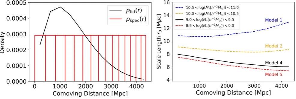
The left panels of Fig.1and Fig.2show the assumed redshift and comoving distance distributions. The black line shows the redshift distribution of the photometric sample and the red bins those of the spectroscopic sample. The right panels of Fig.1 and Fig.2 plot the scale length models of our mock galaxies. The redshift distribution covers a relatively small redshift range up toz <1.5 that is designed to ensure that the assumptions we impose on the redshift evolution of the galaxy-dark matter bias and the power law exponent can be expected to be valid to a good degree. We refer to the following sections §2.4and §2.5for a more detailed discus-sion of these assumptions. We picked a tailed distribution to ensure that our methodology is tested to be robust against cross-correlation measurements with very different signal-to-noise levels. We note however that the particular shape of the photometric redshift dis-tribution does not influence our results on a fundamental level, as we parametrize the photometric redshift distribution using a logis-tic Gaussian process on the (log) histogram bins, which is a very flexible non-parametric approach.

It has to be noted however, that the redshift binning of the spectroscopic sample can introduce an undesired smoothing effect, if these bins are chosen to be too large. For more peaked distri-butions, we therefore might have to consider a finer binning. This effect has been studied inRau et al.(2017), where recommendations about bin width selection, as well as on methods to detect and cor-rect the oversmoothing effect are described. Since our distribution is quite smooth, we expect that our binning scheme is fine enough to capture the structure of the distribution well.

The redshift evolution of the scale length models has been ex-tracted fromSpringel et al.(2018, Fig. 13)4_{. The redshift evolution}

of the exponentγis less dependent on stellar mass as discussed in Springel et al.(2018). For simplicity we therefore choose a common function for these samples that corresponds to the stellar mass bin of Model 5 in Fig.1, i.e. 8.5<log(M∗[h−2M])<9.0. The

dif-ferent scale length models correspond to the stellar mass ranges of the different galaxy samples that we want to consider in this work. In the following we will denote these models with the numbers quoted in the plot. Since we will compare different combinations of galaxy-dark matter bias models for the spectroscopic and photo-metric samples, we will use different scale length factor models for

4 _{We extract these functions directly from the paper plots using the} Web-PlotDigitizer softwarehttps://automeris.io/WebPlotDigitizer/.

each sample. As the redshift, or comoving distance, evolution of the scale factor cannot be measured directly for the photometric sample, we need to parametrize our uncertainty in this quantity.Matthews & Newman(2012) use a constant factor to correct the scale length models from the measured spectroscopic sample to match the pho-tometric one, i.e.r₀,spec(z) ∝r₀,phot(z). However we found that a

constant shift∆, i.e.r_0,spec(z) = ∆+r_0,phot(z) provides a better

fit to offset the spectroscopic scale length model (Model 5) to the assumed photometric scale factor model (Model 4). Furthermore we would like to study more complicated cases, where the differ-ence in the photometric/spectroscopic scale length models is not a simple offset, but depends in a more complicated manner on the comoving distance. This motivated us to parametrize the comoving distance-dependence of the scale length as Chebychev polynomials

r_0,pp(r)=

M

Õ

i=0

∆iTi(r) (14)

where theTi(r)are given by the recurrence relation

T₀(r)=1 (15)

T₁(r)=r (16)

Tn+1(r)=2r Tn(r) −Tn−1(r). (17)

If the coefficients of the higher order termsTifori>0 are the same

for the spectroscopic and photometric samples, this parametrization is equivalent to the previously discussed fit between Model 5 and 4.

We found that the expansion in Chebychev polynomials con-verged rapidly to the true function. By the properties of this basis, omitting higher order terms in this expansion leads to an intrin-sic sparsity in the approximation and they provide good fits to the scale length for M = 2. The constant offset∆then corresponds

to the∆₀ parameter in this expansion. We note that we use the

Chebychev expansion only as a way to interpolate the comoving distance-dependence of the scale length. It is no substitute for a physically-motivated galaxy-dark matter bias model.

2.3 Modelling the Covariance Matrix

The following section describes the modelling of the theoretical covariance matrix. The previous section used a simplified modelling of the angular correlation function. Since computational speed and modelling simplicity is not an advantage for the modelling of the covariance matrix, we use a more accurate approach here. We model the covariance matrix of the angular correlation functions binned in angular binsi, jfor the redshift binsaandbby transforming the covariance matrix of the corresponding angular correlation power spectra for redshift binsaand bas (see e.g.Crocce et al. 2011; Salazar-Albornoz et al. 2017)

Σ(a,b),(i,j)= Õ

l≥2 _2`+1

4π 2

h bL_`ibLjΣ

(a,b)

l,l0

i

, (18)

whereΣa,b

l,l0 denotes the covariance matrix of the angular correlation

power spectra for a pair of redshift binsaandband

b Li_`= 2π

∆Ωi

1 2`+1L˜ ˜

L=L`−₁

cos(θi

R)

−L`+1

cos(θi

R)

−L`−1

cos(θi

L)

+L`+1

cos(θi

L)

,

Figure 1.Left:Redshift distribution of the background sample and spectroscopic tophat functions.Right:Evolution of the scale length as a function of redshift. We omit a ‘Model 3’ here that would correspond to the stellar mass interval between Model 2 and Model 4 and can be found inSpringel et al.(2018, Fig. 13). We do not use this stellar mass bin here, but still want to indicate with the numbering that there is a galaxy population between those shown here.

Figure 2. Left:Distribution of comoving distance of the background sample and spectroscopic tophat functions.Right:Evolution of the scale length as a function of comoving distance.

are Legendre polynomialsL`(x)binned in the respective angular

binsior j. Hereθi_Landθi_Rdenote the left and right edges of the angular bins and∆Ωithe solid angle integral defined in Eq. (10).

We model the covariance matrix between two angular correlation power spectra, that correspond to a pair of redshift bins(i,j)and (k,l)as

Σ(₍k,l)

i,j)(`)=A(`)

¯

C(i,k)(`)C¯(j,l)(`)+C¯(i,l)(`)C¯(j,k)(`) , (20)

which neglects correlations between neighboring angular modes` and non-Gaussian contributions. The cosmic variance factor

A(`)= δ`,` 0

(2`+1)f_sky (21)

is inversely proportional to the fractional sky coverage f_sky and ¯

C(i,j)(`)denotes the shot noise contribution to the angular power

spectra

¯

C(i,j)(`)=C(i,j)(`)+δi,j

¯

ni_g . (22)

The shot noise ¯ni_gdenotes the number of galaxies per steradian in the respective sample. The correlation power spectrum of a cosmo-logical density field, e.g. the density field of galaxy positions or the corresponding field of galaxy shapes in lensing, can be defined as (e.g.Kirk et al. 2015)

C_`i,j= 2 π ∫

Wi(`,k)Wi(`,k)k2P(k)dk (23)

whereP(k)denotes the matter power spectrum andWi(`,k) are

weighting functions that ‘project’ the matter power spectrum along the redshift dimension. For galaxy clustering the weighting function is defined as

W_clus(`,k)=

∫

bg(k,z)n(z)j`(kr(z))D(z)dz (24) wherebg(k,z)denote the (potentially) redshift and scale dependent

galaxy-dark matter bias,n(z)denotes the photometric redshift

dis-tribution,j`(kr(z))denote the spherical bessel functions andD(z)

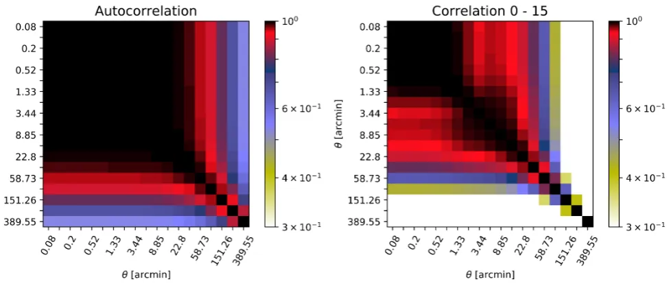
Figure 3. Correlation matrix of angular correlation functions for the auto correlation of the photometric redshift distribution (Left) and cross-correlation between the photometric redshift distribution and the last spectroscopic tophat bin (Right). The bin sizesand colorbarare spaced logarithmically.We set a

lower limit on the correlation coefficients|ρi,j|<0.3 in this plot for better visibility of structure and consistency between the two panels. Accordingly, angular

bins withθ >1◦_{in the right panel are only weakly correlated with sub-degree scales with a correlation coefficient|ρ}

i,j|<0.3.

function takes the form

W_lens(`,k)=

∫

q(z)j`(kr(z))D(z)dz, (25)

whereq(z)denotes the lensing weight

q(z)=3H

2 0Ωm

2c2 r(z)

a(z)

∫ r

r_hor

dr0n(r(z0)) r(z 0

) −r(z)

r(z0)

!

, (26)

wherea(z)is the scale factor evaluated at redshiftzandr_horis the comoving horizon.

The cosmological parameter values and forecast assumptions made in this work are listed in Tab. 2and the assumed redshift distributions are shown in Fig.1. The assumptions on number den-sity and sky coverage are selected in analogy toKirk et al.(2015) and would correspond to a DES Y5-like survey. However the red-shift distribution covers a smaller redred-shift range, as discussed in the previous section. This implies that our signal-to-noise will likely be overestimated, which will make systematic biases due to a mis-specified redshift dependent galaxy-dark matter model more sig-nificant, compared with the statistical error budget. We reiterate that we do not intend to forecast the performance of a particular survey, but rather to test the robustness of our redshift inference to a redshift-dependent galaxy-dark matter bias mis-specification. We use the cosmosis5 (Zuntz et al. 2015) software to estimate the non-linear matter power spectrum for these parameters and the ‘LimberJack’ code6 _{to calculate the galaxy angular power}

spec-tra, where we use the Limber approximation for ` > 60 and the exact calculation for smaller modes (see e.g.Thomas et al. 2011, §4). We perform the summation in Eq. (18) up to ` = 5000 to ensure convergence. We note that the covariance matrix of the an-gular correlation power spectra exhibits correlations between the auto-correlation of the photometric bin and the cross-correlations

5 _{https://bitbucket.org/joezuntz/cosmosis/wiki/Home} 6 _{https://github.com/damonge/LimberJack}

with the spectroscopic tophat bins. These correlations are largest for low angular modes and decrease for larger modes. As these cross-correlations are typically ignored in similar cross-correlation analyses, where the auto-correlation and the cross-correlations are fit individually (e.g.Newman 2008b;Matthews & Newman 2010), we will only consider the diagonal component of the covariance matrix for simplicity. However we do stress that these cross terms have been used in previous applications of the cross-correlation technique (e.g.Matthews & Newman 2012) and should be included in a practical application to data.

The left panel of Fig.3shows the correlation matrix of the angular correlation function for the example of the auto-correlation of the photometric sample. Similarly the right panel of Fig.3shows the correlation matrix of the angular correlation function for the cross-correlation between the photometric sample and the last spec-troscopic tophat bin. We see in both panels, that the correlation of sub-degree angular scales is very high and decreases for correlations on larger angular scales. We note however that this result strongly depends on the impact of shot noise on the covariance, and there-fore on the considered galaxy sample.Note that in order to better resolve the structure of the correlation matrix on small scales, we decrease the color range by setting a lower limit on the correlation coefficients in the plot to|ρ_i,j|>0.3.

Due to the high correlation on sub-degree scales, we consider a single angular bin fromθ ∈ [0.1,1.0]arcmin, which is in the

regime where the Limber approximation (see §2.1) is quite accurate. These scales are also comparable to the angular bins within 0.06−

6[arcmin]that have been used inMatthews & Newman(2010). We

Table 1.Cosmological parameter values in analogy toSpringel et al.(2018) and forecast assumptions for a photometric and spectroscopic survey similar toKirk et al.(2015).

Ωm 0.3089 h 0.9774 fsky 0.12

Ωb 0.0486 σ8 0.6774 nphotg [arcmin−2] 10

ΩΛ 0.6911 ns 0.9667 nspecg [arcmin−2] 0.56

2.4 Generating the mock data vector

As discussed in the previous section, we find a large correlation between angular correlation function bins on small angular scales. Similar to Ménard et al.(2013) we therefore generate our mock data for the photometric galaxy angular auto- and cross-correlations with the spectroscopic tophat bins using a single angular bin within

[0.1,1.0]arcmin following Eq. (11).

This correlation function is generated assuming a redshift-dependent scale length and power spectrum exponentγ(r)model

that we discretize within the comoving distance bins shown in Fig.1 as described in §2.1. We note that the binning of the redshift dis-tribution and the discretization ofr₀(r)andγ(r)are performed in

comoving distance. We reiterate that the creation of the covariance matrix uses a more accurate modelling of the correlation functions. Since the software we use to obtain galaxy angular correlation power spectra in §2.3assumes a redshift distribution, we transform the histograms defined as comoving distance distributions p(r) into

redshift spacep(z)according top(z)=p(r)|dr/dz|. Since the

his-togram assumes a uniform distribution in comoving distance, this transformation leads to tilted histogram bins and tophat functions. Since this is an artifact of the histogram discretization, we re-bin at the histogram midpoints for plots like Fig.1. However, to ensure consistency with the modelling of the angular correlation function data vector, we transform all comoving distance tophat functions and histogram bins into redshift space without re-binning before the angular correlation power spectra are obtained.

We reiterate that the scale length model strongly varies as a function of stellar mass, while the model forγ(z)is quite similar

for different galaxy populations within the redshift range (z<1.5) considered in this work. Thus, while we will use different scale length models in our mock data vector, we will choose the same model forγ(r)that corresponds to Model 5 in Fig.1.

We note that the long-tailed shape of the photometric redshift distribution shown in the left panel of Fig.1ensures that the sam-pling tested in the following sections has to prove its robustness against significant variations in signal-to-noise in the parameters that describe the photo-z distribution. As this work does not consider inhomogeneous spectroscopic samples, i.e. spectroscopic samples that consist of very different galaxy populations across redshift, we do not extend our redshift range beyondz >1.5, where a realistic spectroscopic sample will consist of high-redshift quasar samples with quite different clustering properties compared with the rest of the sample.

The modelling of the data vector also uses Eq. (11), however the scale length offset∆₀(see §2.2) is treated as a random variable.

In §4.2we study the effect of biased scale length models on the accuracy of the reconstructed photo-z distribution.

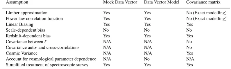
2.5 Summary of modelling assumptions

In the following we summarize the modelling assumptions made when generating the mock data vector, the modelling of this data

vector and the modelling of the covariance matrix. These points are also listed in Tab.2for easy reference. We list the assumption in the first column and list if this affects the generation of the mock data vector, the modelling of the data vector and the modelling of the covariance matrix in the subsequent columns.

Limber Approximation and Power Law correlation function We use the Limber approximation to model the angular correlation functions within a single angular bin ofθ∈ [0.1,1.0]arcmin. The

Limber approximation in combination with a power-law correla-tion funccorrela-tion is the basis of many cross correlacorrela-tion methods (e.g. Newman 2008b;Matthews & Newman 2010;Ménard et al. 2013). We use this assumption in both the generation and modelling of the data vector. This analytical model allows us to quickly evaluate the correlation functions, which is very beneficial for efficient sam-pling. The Limber approximation can be expected to be accurate on the percent level within the considered scales (see e.g.Simon 2007). We expect that deviations from the power-law correlation function can introduce a larger source of modelling bias, especially on smaller scales and high redshiftz>1.5, where scale-dependent galaxy-dark matter bias will become important. For the modelling of the covariance matrix, we do not assume a power law correla-tion funccorrela-tion and do not impose the Limber approximacorrela-tion. Since the advantages of the Limber approximation, i.e. convenient mod-elling and computational speed, do not affect the generation of the covariance matrix, we use the more exact treatment here.

Galaxy-Dark Matter bias While we investigate the effect of a redshift-dependent galaxy-dark matter bias, we do not address the issue of a possible scale dependence. We neglect the stellar mass de-pendence of the correlation exponentγand use the same model for all galaxy samples. Furthermore we assume linear biasing through-out the paper. These assumptions are made for the creation of the mock data vector and its modelling.

Since we use the full modelling of the power spectrum for the modelling of the covariance matrix, we need to convert the scale length and power spectrum exponent into a redshift-dependent galaxy-dark matter bias model according to Eq. (13). We use the aforementioned ‘global’ correlation exponent model, as well as the assumption of linear biasing.

Covariance modelling The modelling of our covariance matrix in-cludes both the shot noise contribution and cosmic variance. How-ever for simplicity we neglect correlations between angular modes and cross terms between the auto- and cross-correlations of the data vector. As shown in Fig.3, correlations between auto- and cross-correlations become important at small angular modes, i.e. larger scales. A more complete modelling should therefore include these terms.

like-Table 2.Summary of modelling assumptions in the generation of the data vector, modelling of the mock data vector and modelling of the covariance matrix.

Assumption Mock Data Vector Data Vector Model Covariance matrix

Limber approximation Yes Yes No (Exact modelling)

Power law correlation function Yes Yes No (Exact modelling)

Linear Biasing Yes Yes Yes

Scale-dependent bias No No No

Redshift-dependent bias Yes Yes Yes

Covariance between` N/A N/A No

Covariance auto- and cross-correlations N/A N/A No

Cosmic Variance N/A N/A Yes

Account for cosmological parameter dependence N/A No N/A

Simplified treatment of spectroscopic survey Yes Yes Yes

lihood of the large scale clustering measurement, given the small scale data vector. This is left for future work.

Galaxy Sample Selection In this work we use a very simplistic se-lection of galaxy samples based on their stellar mass. Furthermore we assumed that we will be able to control the error contribution from uncertainties in the galaxy-dark matter bias of the spectro-scopic sample to sufficient accuracy to not significantly widen our redshift posteriors. In future applications to data, we will have to include the spectroscopic measurement into the data likelihood and incorporate the complex galaxy selection function of spectroscopic surveys into the modelling. Especially at higher redshift, we must account for inhomogeneous galaxy populations in the spectroscopic reference sample and a more complex galaxy-dark matter bias model than presented in this work.

3 STATISTICAL MODELLING

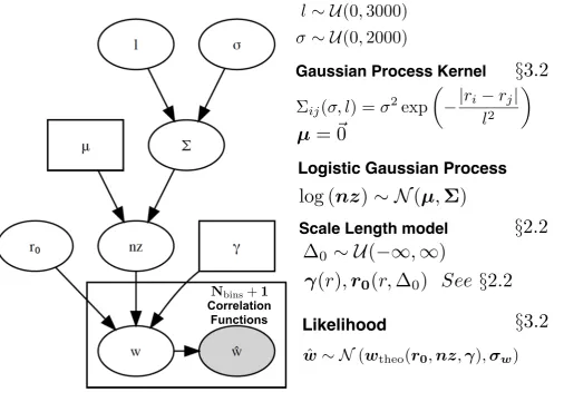
In this section we will introduce our statistical model and discuss our sampling methodology. We use a graphical notation in the form of a directed graphical model shown in Fig.4. This diagram summarizes the dependency between the different random variables in a concise manner.

3.1 Directed Graphical Models

A directed graph, such as Fig.4, illustrates the dependency between different random variables schematically as a set of boxes or circles that are connected with arrows. Boxes denote variables with fixed values, circles represent random variables and shading represents a known random variable, e.g. a data vector. Arrows represent de-pendencies between these variables. For example, if two random variablesaandbare connected by an arrowa→b, they are not

independent, i.e.p(a,b)_,p(a)p(b)and we need to define the

con-ditional probabilityp(a|b)of a random variableagiven the value ofb. The likelihood is shown in a box that represents the dimension of the random variable, in our case of the data vector ofN_bins+1 angular correlation functions. A filled circle within such a box thus represents the measured data, i.e. the angular correlation function measurementwb, where the dimension is specified in the larger box. The modelled data vector is again a random variable, as it depends on a set of parameters that are themselves random variables. Ac-cordingly the model for the measured data, i.e.w, is shown as an

open circle, where the model depends on a set of model parameters. The boxed nodes shown in Fig.4therefore represent the likelihood termL=p(

b

w|w), i.e. the probability of the data given the model.

In the following we will describe the different components of the particular model shown in Fig.4.

3.2 Logistic Gaussian processes for Redshift Inference

We model the redshift distribution of the photometric sample as a histogram in comoving distance shown in Fig.1, where the his-togram bin midpoints are placed at the position of theN_bins spec-troscopic tophat bins that are shown in red. We note that the bin sizes are selected such that they span equal-sized bins in redshift of size∆z=0.1. We discretize the photometric redshift distribution, the distance dependent scale factorr₀(r)and the exponentγ(r)on

this grid to model the angular correlation functions as described in §2.1. The data vectorwbtherefore consists of the auto-correlation of the photometric redshift bin and the cross-correlations between the photometric redshift bins and the spectroscopic tophat distributions. In this paper we will treat each bin height of the photometric sample, and the first order term in the Chebychev expansion (‘scale length offset∆₀’), as random variables. We fix the scale length model of

the spectroscopic sample to its fiducial value and marginalize over the scale length offset∆₀of the photometric scale length model.

We note that the data covariance of the cross-correlation mea-surements implicitly contains our uncertainty in this parameter via the spectroscopic auto-correlation terms in Eq. (20). The scale length models of the spectroscopic and photometric samples are strongly degenerate via the linear biasing assumption Eq. (12). For the considered data vector it is therefore practical to fix these spec-troscopic terms, that will likely be constrained to good precision by future spectroscopic surveys like DESI. A more complete treatment would explicitly break this degeneracy by including the measure-ment of the spectroscopic correlation functions into the data vector. We leave this for future work.

Likelihood specification We assume a Gaussian likelihood for the data vectorwb

p(_bw|w_model,C)=

Nbins+1 Ö

i=1

N (w_bi|wmodel,i, σw,i), (27)

where the product runs over the auto-correlation and theN_bins cross-correlations with the spectroscopic tophat bins. The modelling of the angular correlation function is then given by Eq. (11).

l

⇠ U

(0

,

3000)

⇠ U

(0

,

2000)

Gaussian Process Kernel

Logistic Gaussian Process

Scale Length model

Likelihood

§

2

.

4

.

2

§

2

.

4

.

2

§

2

.

2

⌃

ij

(

, l

) =

2

exp

✓

|

r

i

r

j

|

l

2

◆

µ

=

~

0

log (

nz

)

⇠ N

(

µ

,

⌃

)

ˆ

w

⇠ N

(

w

theo

(

r

0

,

nz

,

)

,

w

)

0

⇠ U

(

1

,

1

)

(

r

)

,

r0

(

r,

0

)

See

§

2

.

2

Correlation

Functions

N

+

1

§

3

.

2

§

3

.

2

Figure 4. Graphical representation of the hierarchical logistic Gaussian process model. Empty/filled circles show unobserved/observed random variables and boxes denote fixed values. Arrows illustrate relationships between the variables. The boxed area represents a joint likelihood of angular correlation function measurements. This includes the autocorrelation of the photometric redshift distribution and the cross-correlations with the spectroscopic tophat bins. We list a summary of the model in the right column. Note that vector-valued quantities are shown in bold face. We also refer to the corresponding paper sections for more information. HereU(x,y)andN(µ, σ)respectively denote a uniform distribution in the limits[x,y]and a normal distribution with meanµand standard

deviationσor covarianceΣin the multivariate case.

Prior specification We set a logistic Gaussian process prior on the N_bins photometric redshift histogram heights denoted as the empty circle ‘nz’ in Fig.4. Accordingly, the logarithm of theN_bins dimensional vector of histogram heights log(nz)is assumed to be

drawn from a multivariate normal distribution with mean vectorµ andN_bins×N_binsdimensional covariance matrixΣ

log(n z) ∼ N (µ,Σ). (28)

The advantage of using a logistic Gaussian Process prior – in con-trast to alternatives such as the Dirichlet or flat priors – is that it opens the possibility of encoding knowledge of the shape and smoothness of the redshift distribution in the covariance function. This is however optional, and the Gaussian can be chosen to be very uninformative.

As described in the following, we can jointly marginalize over the parameters that describe the redshift distribution and the scale length model, which accounts for the degeneracy between the pa-rameters of the redshift distribution and the galaxy-dark matter bias model. Furthermore, the logistic transform guarantees positivity in

thenzposteriors. These aspects are an advantage over applying a

Gaussian Process interpolation, e.g., on the posteriors from a clus-tering redshift technique.

If not mentioned otherwise, we fix the mean ‘µ’ of the logistic Gaussian process to zero and marginalize over the uncertainty in the covariance matrix. For this we choose the following kernel

Σi,j(σ,l)=σ2exp

−|ri−rj|

l2

, (29)

which is a special case of the Matérn kernel (Rasmussen & Williams 2006), a common choice for Gaussian processes. We also tried the squared exponential kernel, however we found that this choice produced numerically more stable covariance matrices. The two parametersσandlgovern the magnitude of the diagonal compo-nents, as well as the correlation, or smoothness, of the histogram. In our model we therefore add a hierarchy that marginalizes over these parameters using broad uniform priorsl ∼ U(0,3000)and σ ∼ U(0,2000). The units of these parameters are [l] = pMpc

and ‘σ’ are shown in Fig.4in the top hierarchy. As detailed in §2.1, we fix the redshift dependence of the power law exponent ‘γ’ and choose an unrestricted flat prior on the first coefficient of the Chebychev expansion, the ‘scale length offset∆₀’.

3.3 Sampling Methodology

We sample the model shown in Fig. 4 using a combination of Metropolis-Hastings sampling and Elliptical Slice sampling steps.

We use two separate one-dimensional Metropolis-Hastings steps to sample the two parameters that describe the Gaussian Process Kernel, a one-dimensional Metropolis-Hastings step to sample the parameter that describes the scale length model and an elliptical-slice sampling step to sample the parameters that describe the back-ground sample redshift distribution. Since in each of these steps we fix the other parameters fixed, which mimics Gibbs sampling, we will refer to the procedure as ‘Metropolis-Hastings within Gibbs’ sampling. The Metropolis-Hastings sampling approach is described in §3.3.1and the Elliptical Slice sampling method in §3.3.2.We will then detail the concrete sampling implementation in §3.3.3.

3.3.1 Metropolis-Hastings sampling

Assuming a set of random variables θ, Metropolis-Hastings within Gibbs sampling (see e.g. Gelman et al. 2004) iteratively samples from the distribution of each variable θi conditional

on all other variables θ−i, i.e. p(θi|θ−t−i1,D), where θt

−1 −i =

θt

1, . . . , θti−1, θ

t−1

i+1, . . . , θ t−1

d

.Here D denotes the data vector,t counts the number of iterations andidenotes the index of the vari-able that is currently updated. If this conditional distribution is not known, we draw samples for a new parameterθ?_{given a previous}

state of the parameterθt−1_{from a proposal distributionJ}

t(θ?|θt−1).

These samples are then accepted with probability

r= p

(θ?

i |θ−i,D)/Jt(θ?i|θt

−1

i )

p(θt−1

i |θ−i,D)/Jt(θt

−1

i |θ?i)

. (30)

We can connect the posterior probabilities p(θ_i|θ_−i,D)via

Bayes rule with the likelihoodp(D |θ_i, θ−i)and the priorp(θi)as

p(θ_i|θ_−i,D) ∝p(D |θ_i, θ_−i)p(θ_i|θ_−i). (31)

We select a normal distribution as the proposal distribution Jt(θ?_i|θt_i−1)=N (θ?_i |µ=θ_it−1, σ), where we center the Gaussian

at the previously proposed valueθt−₁

i and tune the standard

devia-tionσsuch that we obtain acceptance rates between 20%-30% for the respective parameters. Since this distribution is symmetric, it cancels in Eq. (30).

We note that samples are always accepted (r =1) if we use

the conditionalsp(θ_i|θt₋−1

i ,D)in Eq.30as the proposal

distribu-tion. This special case is known as Gibbs sampling and can be used for a restricted set of models, typically complex conjugate models, for which we can obtain an analytical distribution. We note that the Metropolis-Hastings steps described do not have to be one-dimensional (single parameter updates), but rather can use multidimensional proposal distributions.

Furthermore we note that the sampling algorithm used to update each parameter does not have to employ the Metropolis-Hastings scheme, but can use other sampling approaches. The it-erative update of the conditionals then gives the possibility to use different sampling algorithms as ‘building-blocks’ for a combined sampling scheme. We will describe an alternative scheme in the

next section andrefer the interested reader toGelman et al.(2004) for a more detailed description of the Metropolis-Hastings sampling methodology.

3.3.2 Elliptical Slice Sampling

Slice sampling samples from a densityp(z)by considering the area

under the density function represented by the joint density of z

and an auxiliary variableu. After sampling from this joint density,

samples of the variableuare dropped to obtain samples fromp(z).

Following e.g.Dittmar(2013) we can write:

p(z)=

∫ pˆ(z)

0

1

Zp_ˆ

du= ∫

p(z,u)du, (32)

where ˆp(z)does not have to be normalized andZp_ˆis a normalization

constantpˆ(z)

Zpˆ =p(z). The joint distribution is then given as

p(z,u)=

(

1/Zp_ˆ if 0≤u≤pˆ(z)

0 otherwise . (33) Using the same methodology introduced in the previous sec-tion, we first sample fromp(u|z) usingu∼ U [0,pˆ(z)]and then

fromp(z|u)represented as a sample from the ‘slice’{z:u<pˆ(z)}.

While the first step of slice sampling is trivial, the second often involves starting with an initial sample and selecting a larger proposal region, determined by a step size parameter, that contains both the sample and the slice. Then an initial sample is drawn from that region. If this initial sample lies outside the target slice, the size of the proposal region is reduced and the procedure is repeated. Concretely we note that it is still necessary to select a step size parameter, to define the proposal region.

Elliptical Slice sampling is a variant especially geared towards target distributions of the form

p?(θ)= 1

Z p(D |θ) N (θ,0,Σ), (34)

whereθ denotes the free parameters of the model, N (θ,0,Σ) is

a Gaussian prior andp(D |θ)describes the likelihood. In contrast

to classical slice sampling, the proposal region is now an ellipse defined by a sample from the priorν∼ N (ν,0,Σ)and the current

parameter stateθt−_1:

θ∗_=θt−1_{cos(α)+νsin(α). (35)}

Here,α describes the position on this elliptical proposal region. Since the initial sample is drawn from the full ellipse, it is not nec-essary to select a step size. The sampling and shrinking operations are then performed in analogy to the classical slice sampling algo-rithm. We refer the interested reader toMurray et al.(2009) for a more detailed description of the method.

3.3.3 Sampling the Logistic Gaussian process

Starting from the top end of Fig.4, we use three main Metropolis-Hastings steps to sample the hyperparameters of the logistic Gaus-sian process covariance, the (log) histogram heights of the pho-tometric redshift distribution and the scale length offset∆₀ that

describes the scale length model. The sampling of the hyperpa-rameterslandσis performed in two separate Metropolis-Hastings steps. Then, we sample the histogram heights using Elliptical Slice sampling. In the third Metropolis-Hastings step we sample the scale length offset∆₀. In each of these steps we hold the parameters that

We note that the parameters that describe the histogram heights and scale length model can be quite correlated and Elliptical Slice sampling allows us to take larger steps along the degeneracy direc-tion, which leads to better sampling performance for the logistic Gaussian process model. We further note that this methodology does not require gradients, which will not be available if we sample over a likelihood, which models the correlation functions in terms of cosmological parameters.

In the following we will discuss how we construct a prior on the redshift distribution from a Bayesian histogram of sampled red-shift values. In the experiments we performed in the next section we found that Metropolis-Hastings sampling performed better in combination with this redshift prior. The reason is that this prior weakens the correlation between the aforementioned parameters, in which case Metropolis-Hastings sampling becomes more efficient. We therefore used Metropolis-Hastings sampling steps for the in-dividual log histogram heights instead of Elliptical Slice sampling. We note that this might not be an optimal choice for different priors and data likelihoods.

3.3.4 Informative Prior on the Redshift distribution

To set aninformativeprior on the redshift distribution, we require an independent set of data that constrains the histogram bins repre-sented as the logistic Gaussian process. This information will typi-cally come from photometric redshift estimation based on template fitting or machine learning, that constrain the redshifts of individual galaxies. A prior on the population of redshift values can therefore be represented as a Bayesian histogram and samples can be drawn from a Dirichlet distribution given the counts of galaxy redshifts in the respective histogram bins. The distribution over the set of histogram heightsnzb is therefore given as

b

nz∼Dir(Φ+_bc), (36)

where Dir denotes the Dirichlet distribution and Φits parameter

that is set to a unity vector to represent a flat prior. The vectorbc denotes the counts of galaxy redshifts in the respective histogram bin. Herebcis a vector of lengthM, whereMdenotes the number of histogram bins. Accordingly, a sample nzb from the Dirichlet distribution is anMdimensional vector of histogram heights. If the sample size is large, i.e. if each element ofbcis high, the scatter of new samples around the mean histogram heights is small. However if there are very few galaxies in the sample, the Dirichlet distribution will sample around this mean value of histogram heights more broadly. Since the treatment of photometric redshift error in the context of machine learning or template based photometric redshift techniques is beyond the scope of this paper, we will use a lower bound on the prior width by assuming true redshift values for all galaxies in the photometric dataset.

For our case, we find that the logarithm of these sampled redshift histogram heights can be approximated as a multivariate normal distribution to sufficient accuracy for our purposes. For this we use the sample mean and covariance estimated on a large number (>108) of (log) Dirichlet samples for our approximation. This multivariate normal distribution can then be readily used as a prior distribution for the logistic Gaussian process model.

3.4 Model Evaluation

In many practical application of inference there will be a level of uncertainty in the underlying modelling and, as a result, a level

of ambiguity between reasonable model choices. It is therefore of paramount importance to compare these models efficiently and combine them if various models provide equally good descriptions of the data. We evaluate and compare the models using goodness of fit statistics and the expected biases in the Lensing convergence power spectrum. The latter is especially useful as it allows judgment about the possible impact of residual photometric redshift errors on the weak lensing measurement, which is the primary cosmological probe to test theories of dark energy in the context of large area photometric surveys.

3.4.1 Information Criteria

In classical statistics the maximum of the log-likelihood is of-ten penalized by the number of free parameters in the model, to measure the ‘goodness of fit’ and avoid the risk of specifying too many parameters (‘overfitting’). This approach, represented by the Akaike information criterion (AIC;Akaike 1973), has the disadvan-tage in the Bayesian analysis, that it will not change with different prior choices that clearly affect model complexity and posterior. In this work we will therefore use the Deviance Information Criterion (DIC;Spiegelhalter et al. 2002) that provides an extension of the AIC towards the Bayesian paradigm.

We use the definition of the DIC based on the predictive den-sity7(Gelman et al. 2013) as

DIC=logp

D |bθBayes −pDIC (37)

where D denotes the data vector and pD |bθBayes

denotes the likelihood evaluated at the posterior expectation

b

θ_Bayes=E[θ|D]. (38)

Model complexity is then penalized as

p_DIC=2 var_Postlog(D |θ), (39)

where varPostlog(D |θ)denotes the posterior variance of the

likeli-hood. More complex models will have a larger posterior variance due to their additional degrees of freedom in parameter space. As both terms in the DIC are evaluated with respect to the posterior, its value will depend on the choices of prior.

We note that an alternative to this approach (that is com-monly used in cosmology) is a model selection using the marginal likelihood, or evidence, for a modelM_i from a set ofCmodels

M={M₁, . . . ,M_C}:

p(D |M_i)=

∫

p(D |θ,M_i)p(θ|M_i)dθ , (40)

whereθare the model parameters andDrepresents the data. While

we could have used multimodel inference techniques likeBarker & Link(2013) on our previously fitted chains to estimate marginal likelihood for all the models used in this paper, we decided to use the DIC criterion for its simplicity and computational speed.

We note, however, that a Bayesian information criteria like the DIC can have advantages when averaging over multiple models becomes necessary, or if multiple models need to be ‘scored’ based on their ‘goodness of fit’. The evidence can be used to ‘weight’ the posterior constraints for different models in the case where the true

model is known to be in the model setM. If this is not the case,

this approach will select the single ‘best fit’ model in the large data limit. In cases where the true model is not part of the model set, techniques based on information criteria or ‘stacking’ techniques (e.g.Gelman et al. 2013) may be more suitable. Furthermore the evidence can be dependent on prior choices (Gelman et al. 2013), which may lead to specification problems especially if the model set is incomplete. Thus, while our primary motivation for using the computationally more efficient DIC criterion is computational speed and simplicity, we would like to highlight the usefulness of information criteria, especially if we expect systematic modelling errors that could cause an incomplete model set.

3.4.2 Bias in lensing convergence power spectrum

To be able to better evaluate the significance of photometric redshift biases, we evaluate the quality of the reconstructed photometric redshift distribution in terms of the expected relative bias in the lensing convergence power spectrum

∆_rel=

b

C_{`</sub>fid.−Cb<sub>`}bias b

C_`fid. , (41)

whereCbdenotes the binned lensing power spectrum

b C`= 1

N_` Õ

`

C`, (42)

andN` denotes the number of integer angular modes. Here,Cb<sub>`</sub>fid. denotes the lensing convergence power spectrum obtained using the unbiased, fiducial, redshift distribution.Cb<sub>`</sub>biasdenotes the photomet-ric redshift distribution obtained assuming the (potentially) biased galaxy-dark matter bias model in the inference. We choose to bin the angular correlation power spectra` ∈ [10, `<sub>max</sub>], where we select `max =3000 in analogy toKirk et al.(2015). We compare the

re-sulting systematic biases with the expected statistical measurement error from a weak gravitational lensing measurement with the speci-fications given in Tab.2and a shape noise ofσ=0.23 comparable

withKirk et al.(2015). The error in the binned measurement is then

σ(Cb`)= 1 N`

v u t

Õ

`

2

(2`+1)f_sky

C`+ σ

2

2ng

2

, (43)

which implements Eq. (20) with a different, weak gravitational lensing specific, shot noise term. Eq. (43) also includes the cosmic variance contribution to the covariance matrix, that is inversely proportional to the fractional sky coverage f_sky. Neglected are the covariance between the different modes`. This is done in analogy to other forecasts likeKirk et al.(2015). The 1σ error in∆_relis

then given as

σ∆_rel= σ(Cb`)

d C_`fid

(44)

We note that this simple metric does not substitute an ac-curate forecast that evaluates the impact of photometric redshift bias on cosmological parameter inference. This would require a tomographic analysis that is representative of modern surveys like DES or LSST, which is beyond the scope of this work. However, if the mean systematic bias in the reconstructed lensing convergence power spectrum is significantly below the statistical error budget given in Eq. (43), we can assume that its impact on cosmological

parameters will be small. It therefore allows us to approximately judge the practical implications and relevance of the photometric redshift error on cosmological parameter inference, even without a more precise forecasting exercise.

4 ANALYSIS AND RESULTS

In the following section we investigate the performance of our logis-tic Gaussian process model in recovering the photometric redshift distribution using the cross-correlation likelihood (Eq.27) and test how different scale-length models affect the inference.

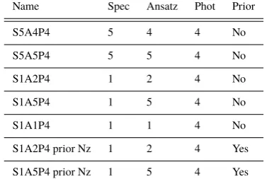
Tab.3summarizes the nomenclature used in our analysis. The first column quotes the name tag of the particular setup, the second column the scale length model assumed for the spectroscopic sam-ple, the third our ansatz for the scale length model of the photometric sample and the fourth column lists the true scale length model of the photometric sample (that is unknown to us in practise). The final column indicates if a prior on the photometric redshift distribution is used. We refer to Fig.1for an overview over the different scale length models. We note that we adapt the covariance matrix of the likelihood to changes in the corresponding galaxy-dark matter bias according to Eq. (13).

4.1 Fiducial Model

In this first section we study a test case where our assumption that the scale length model of the photometric and spectroscopic samples only differs by a constant offset is valid to a good degree. This is the case for example in Model 4 and 5 shown in Fig.1. As can be seen this implies that both samples have similar stellar mass ranges, which would require a spectroscopic survey that does not exhibit an extreme selection towards highly biased tracers. We therefore study this scenario assuming Model 4 as the scale length model of the photometric sample and Model 5 as the scale length model of the spectroscopic sample. As discussed in §2.2, we use a constant offset to parametrize our uncertainty in the scale length, which corresponds to the first (constant) term in the Chebychev expansion. In the following, we will refer to this case as ‘S5A5P4’. To test if the small differences between Model 4 and 5 will introduce biases in our inference, we compare with the results in the absence of systematics. For this unbiased, fiducial test case, we fix the higher order terms of the Chebychev expansion to their true, unbiased, values from Model 4. As before, we will marginalize over an offset in the scale length and will refer to this case as ‘S5A4P4’. Note that this scenario is not the same as assuming scale length model 4 for both the spectroscopic and the photometric sample, because our covariance matrix will assume scale length model 5 for the spectroscopic sample. To simplify the notation, the following will refer to the offset in the scale length as ‘scale length offset∆₀’.

The left panel of Fig.5shows the posterior of the difference between the true photometric redshift distribution and the redshift distribution inferred in these models. All distributions shown in this work have been normalized to unit area. We show the results for ‘S5A4P4’ in grey contours and results for ‘S5A5P4’ in red. The right panel plots the corresponding posterior distributions for the scale length offset∆₀, where the dashed blue line denotes its true

Table 3. Summary of the model nomenclature used in this work. We list the model name, the assumed scale length model (see Fig.1) for the spectroscopic sample, the Ansatz for the scale length of the photometric sample and the true scale length model of the photometric sample. The last column indicates if a prior on the photometric redshift distribution was used.

Name Spec Ansatz Phot Prior

S5A4P4 5 4 4 No

S5A5P4 5 5 4 No

S1A2P4 1 2 4 No

S1A5P4 1 5 4 No

S1A1P4 1 1 4 No

S1A2P4 prior Nz 1 2 4 Yes

S1A5P4 prior Nz 1 5 4 Yes

Table 4.Results of the model comparison between different redshift depen-dent galaxy-dark matter bias models summarized in Tab.3. DIC denotes the Deviance Information criterion (Eq.37),p_DICthe measure of model complexity (Eq.39), ‘Loglike’ denotes the log-likelihood evaluated at the mean of the posterior, i.e. the first term in Eq. (37). ‘Cl Bias’ denotes the relative bias in the lensing convergence power spectrum (Eq.41).

Name DIC Cl Bias Loglike pDIC

S1A2P4 77.85 1.77 95.71 17.86

S1A5P4 81.54 0.26 95.58 14.04

S1A1P4 -2385.84 3.70 -2370.28 15.57

S1A2P4 prior Nz -117.47 0.76 24.31 141.78 S1A5P4 prior Nz 93.30 0.10 101.05 7.75

The[5,95]posterior percentile range of the inferred

photomet-ric redshift distribution assuming the slightly biased case S5A5P4 are largely consistent with the true result, however, as expected, in-consistent for the scale length offset∆₀. We can therefore conclude

that a slight modelling bias in the scale length, or galaxy-dm bias model, has a small effect on the accuracy of the recovered redshift distribution. It has to be noted that we make quite optimistic assump-tions for the photometric and spectroscopic surveys (see Tab.2). For less optimistic assumptions, e.g. a smaller area of overlap between spectroscopic and photometric survey, we can expect the statisti-cal error to be larger. The statististatisti-cal error then quickly becomes even more dominant compared with the small photometric redshift systematic shown in Fig.5.

We note that there is considerable degeneracy between the scale length offset and the redshift distribution, particularly for the low redshift bins where the signal-to-noise ratio in the clustering measurement is large. This is illustrated in Fig.6for the unbiased model S5A4P4, which shows the posterior distributions of the scale length offset∆₀and the first two histogram bin heights of the

pho-tometric redshift distribution. We see that the scale length offset

∆₀and the photometric redshift distribution bin heights are indeed

strongly correlated. For the bins at higher comoving distance, or redshift, this correlation decreases.

In the next section we will discuss a more extreme case, where larger differences in the stellar mass of the photometric and spec-troscopic galaxy population translate into larger differences in the scale length models.

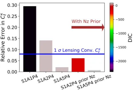
4.2 Impact of biased scale length models

We test the impact of biased scale length models on the redshift dis-tribution inference in a more pessimistic setup: we make the ansatz that the scale length of the photometric/spectroscopic sample is given by scale length Model 4/1 and denote this setup as S1A1P4. As one can see from Fig.1, a simple constant shift in the scale length model is no longer a sound approximation, as both models have a significantly different slope at large comoving distances or high redshift. This can be seen as an extreme case of scale length model mis-specification and we will likely be able to calibrate the model to better accuracy either using simulations or by incorpo-rating information from e.g. galaxy-galaxy lensing (e.g.Prat et al. 2018) in future surveys.

We therefore include a more optimistic setup into this compar-ison. Here we make the ansatz for Models 2/5, that are more similar to the true photometric model (Model 4). This means that instead of fixing the higher order coefficients of the Chebychev expansion to the parameters of Model 1, we fix them to the parameters of Model 2/5. We will denote the Model 1-4 with an ansatz of Model 2/5 as ‘S1A2P4’ and ‘S1A5P4’ respectively. As in the previous section we will marginalize over the constant term in the Chebychev expansion, i.e. the ‘scale length offset∆₀’. Fig.7shows the resulting difference

in the recovered redshift distributions, where the ‘pessimistic’ case of Model 1-4 shows considerable biases that are reduced by S1A2P4 and to better accuracy by S1A5P4. This recovered bias is naturally similar to the fiducial case discussed in the previous section8.

Fig.8compares the relative error in the lensing convergence power spectrum for the different model configurations with the sta-tistical error budget to be expected for the lensing survey defined in Tab.2. The corresponding numbers are listed in Tab.4. We see that model S1A1P4 has the largest error in the convergence power spectrum and is clearly rejected by the DIC criterion. However even though S1A2P4 yields a systematic bias that is larger than the statis-tical error budget, it has a similar DIC as the much better-performing model S1A5P4. This is a result of the degeneracy between different scale length models with the redshift distribution of the photometric sample. To highlight this, we impose a prior on the redshift distri-bution bin heights as described in §3.3.4. The corresponding results for models denoted as ‘Nz prior’ are shown in Fig.8and Fig.7. We see that the inclusion of a prior improves S1A2P4 and S1A5P4 in terms of the relative error in the convergence power spectrum. Most importantly however, the difference in DIC is much larger compared with the case that does not incorporate prior information. The worse S1A2P4 model is now more clearly rejected by the DIC criterion. We note that imposing a prior on the scale length offset∆₀was not

sufficient in our experiments to produce this effect. This is sensible, as the redshift distribution in our setup contains many more degrees of freedom compared with the parametrization of the scale length model. This indicates that combining the clustering measurement with external redshift constraints from e.g. template fitting will be necessary to break the degeneracy between our uncertainty in the redshift-dependent scale factor, i.e. the redshift-dependent galaxy-dark matter bias, and the redshift distribution of the photometric sample.

Figure 5. Posterior distributions for the bin heights of the ensemble redshift distribution of the photometric sample and scale length offset∆₀for the model

with mismatched scale length S5A5P4 (red) and matching scale length S5A4P4 (black/grey).Left:We show the[5,95]posterior percentiles of the difference

between the posterior redshift distribution and the true redshift distribution.Right:Posterior distributions of the ‘Scale length offset∆₀’. The blue dashed line

shows its true value.

1.0045 1.0060 1.0075 1.0090

N

Z1

8.15 8.16 8.17 8.18 ∆0

1.816 1.820 1.824 1.828

N

Z2

1.0045 1.0060 1.0075 1.0090 N Z1

Figure 6. Posterior distributions for the unbiased model(matching scale

length)S5A4P4 for the scale length offset∆₀and the first two photometric redshift bins. The dashed lines denote the true values.

5 SUMMARY AND CONCLUSIONS

We have pres