Deployment of a Competition Sprinter Robot over FPGA Platform with Feedback Control Systems for Velocity and Position



Abstract— This paper describes the development of a sprinter robot for tournament competitions, considering aspects in electronics, mechanical and software. The designed robot reaches a maximum velocity of 2.23 m/s in tournament competitions. The paths it travels consist in closed roads formed by straight lines and curves with a minimum radio of 10 cm. The computer deployment that controls the robot was in FPGA EP4CE22F17C6N (Altera’s Cyclone IV family). It was also used a development card DE0-Nano. The system employs a processor defined in software NIOS II from Altera with peripherals for the handling of the robot, and a control system algorithm in cascade for control. Two secondary loops control the velocity of each motor and a primary loop controls each reference according to the direction and central velocity of the robot. Besides, it was deployed a filter system by software, using the Kalman filter algorithm.

Index Terms— Differential robot, FPGA, Kalman filter, sprinter robot.

I. INTRODUCTION

ORLDWIDE exists a diverse variety of robot tournaments. One of the competition categories concerns to sprinter robots. Robots must travel autonomously in the less time possible through a closed path marked with line, obeying additional rules that can differ according to the competition. These tournaments have as objective to impulse the development of diverse technologies related to robotics. Besides, this poses an important challenge to competitors, because they face real problems with solutions in engineering practices.

As electronic components integrate more functions and are more accessible, complexity level in robots have been increasing, even existing a monotony type legacy in previously presented solutions, leading to the constructions of basic robots. Generally, it is not still common the use of

Manuscript received December 07, 2016.

H. I. Veriñaz is with the Escuela Superior Politécnica del Litoral, ESPOL, Faculty of Natural Science and Mathematics, Campus Gustavo Galindo, Km 30.5 Via Perimetral, P.O. Box 09-01-5863, Guayaquil, Ecuador.

C. R. Martinez was with the Escuela Superior Politécnica del Litoral, ESPOL, Faculty of Electrical and Computer Engineering, Campus Gustavo Galindo, Km 30.5 Via Perimetral, P.O. Box 09-01-5863, Guayaquil, Ecuador.

R. A. Ponguillo and V. Sanchez Padilla are with the Escuela Superior Politécnica del Litoral, ESPOL, Faculty of Electrical and Computer Engineering, Campus Gustavo Galindo, Km 30.5 Via Perimetral, P.O. Box 09-01-5863, Guayaquil, Ecuador.

e-mails: {hverinaz, crmartin, rponguil, vladsanc}@espol.edu.ec

professional techniques. Faster robots, classified according to categories, have development mainly in Japan, Poland, Romania and Latvia.

This paper does not try to submit conclusive ideas or optimal solutions for problems presented in the deployment of sprinter robots. In fact, different fields involved, such as electronics, mechanical or software must consider improvements during development stages. Here is exposed a specific solution focused in software and electronics, deployment that allows to develop new solutions for robots, resulting in increasing the difficulty or competitive level of the tournaments.

II. DESIGN AND DEPLOYMENT

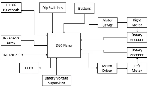
For the construction of the robot is necessary to work in three different design aspects. First, mechanical (or physical) and electronics aspects have to be addressed. Then, software considerations are treated, including the computer deployment with FPGA platform, the Soft-Core processor with its peripherals and the design of control and filtered algorithms using MATLAB, and its deployment over the processor. Figure 1 depicts the system block diagram described in this section.

Fig. 1. Robot’s block diagram.

2.1. Hardware 2.1.1. Mechanical

Although this paper does not focus in the mechanical design, it is necessary to have a notion of the physics that rules the robot behavior in a way the design benefits the

Deployment of a Competition Sprinter Robot

over FPGA Platform with Feedback Control

Systems for Velocity and Position

Herman I. Veriñaz Jadan, Caril R. Martinez Vera,

Ronald A. Ponguillo,

Member, IAENG

, Vladimir Sanchez Padilla,

Member, IAENG

performance of the control algorithm, and therefore the robot movements.

There are several types of locomotion for mobile robots. For a sprinter robot, the most used is the tricycle type and the differential locomotion by two and four wheels.

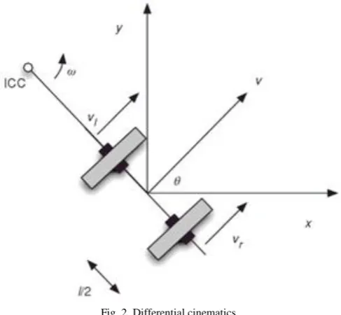
It was used differential locomotion by two wheels, because it represents less difficulty in the mechanical aspect. This type of locomotion has two controlled fixed wheels, one by each side of the robot. Each wheel handles independently to change direction varying the spin velocity in each wheel. It is common to add extra wheels (spherical or with multidirectional spinning) to balance the robot trajectory.

Fig. 2. Differential cinematics.

Listed below are some details for the physical design:

 Low gravity center, to diminish the risk that the front of the robot lifts away from the track, which can cause errors in sensors’ readings.

 Low moment of inertia, to increase the angular acceleration, helping to improve cornering movements.

 Low mass, to improve robot acceleration.

 Silicone rubber wheels, to gain the highest possible friction. Wide tires improve traction. Radius depends on the speed to achieve, but designers must realize that more radius, more factors to consider, e.g., robot mass, inertia moment when loading the motor.

 Unification of the chassis and the circuit, since the robot chassis is the same as the PCB, avoiding the electronic deployment on an isolated chassis, in order to get less failure points and a lighter design.

Motors used for the robot are FAULHABER 2224 SR06 [2], with a nominal voltage of 6V reaching an angular velocity of 8,200 rpm without load. Another feature is the

2.1.2. Electronics

Most of the electronic components used correspond to developed modules distributed in two different boards for communication with the DE0 –Nano card through a proper circuit. Among the principal elements are:

 A Bluetooth HC06 wireless module.

 Two motor controllers TB6612FNG Dual Motor Drive Carrier [3].

 A voltage regulator of 5V D24V50F5 with an output current up to 5A [4].

 A voltage regulator of 3.3V LM1117-33.

 Pushbuttons, voltage divisor to measure the battery voltage.

 Additional feeding ports to adapt some types of sensor required for a specific task.

Besides, there are three sensorial components:

1)An array of fourteen optical sensors to distinguish between black and white to identify robot position regarding to the track. Individual sensors Polulu’s QTR-1A were used [5].

2)Rotary encoders [1] to measure and control the velocity of the motors any time. Each engine integrates these encoders.

3)Inertial measurement unit (IMU), compose by a gyroscope, an accelerometer, and a magnetometer, respect to Polulu’s MinIMU-9 v3 [6].

Fig. 3. Final electronic circuit in PCB.

300 mA·h. The first one is used for testing and the second one for competition, this because the 300 mA·h battery has lesser weight and the power supply lasts enough time for a competition situation.

2.2. Software

2.2.1. Computer construction over FPGA

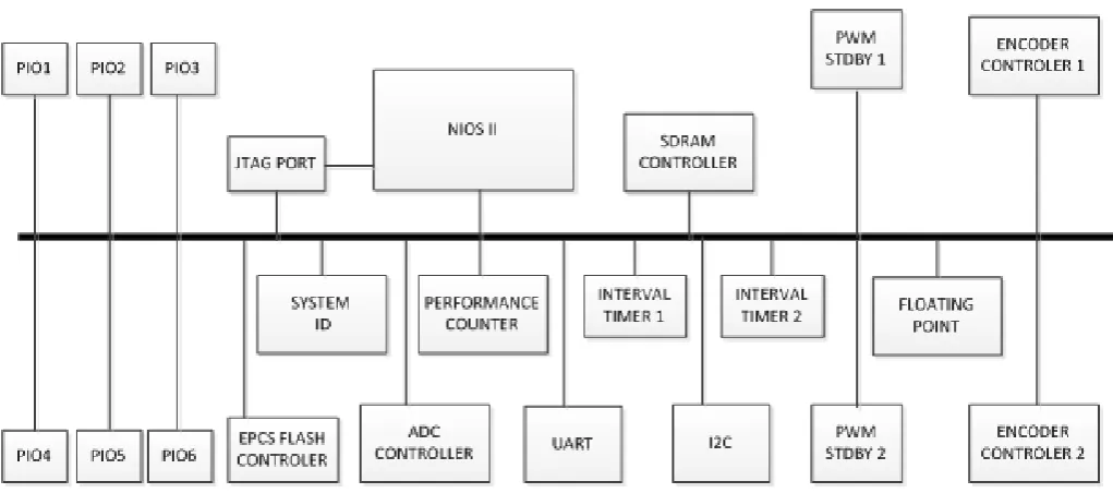
Computer construction was deploy by the Quartus’ Qsys tool, and it took a DE0-nano Basic Computer as reference [7]. Some modifications were made to adapt it to the project [8] [9]. Figure 4 depicts a diagram system with each module used.

2.2.2. Velocity controller

To define robot movement is necessary to specify both angular velocity and linear velocity regarding to its mass centre. It is enough to control the linear velocity in the contact point of each wheel to control both angular and linear velocity of the robot, being this the reason why each motor required a velocity controller. To manage velocity controllers is required an external controller that modifies references according the angular and linear velocity the robot needs.

To identify motor´s transfer function, SDRAM memory of the DE0-nano stored data. Then, a Bluetooth module conveys the data for later analysis with MATLAB.

2.2.3. Filter algorithm

Signals that pass through filter process are signals that comes from rotary encoders, infrared sensors and the gyroscope. Each rotary encoder filters signals independently.

The signal from the infrared sensors and the signal from the gyroscope combine to pass through a filter that fusion both data. Both signals used the Kalman filter algorithm, due to its great impact in estimation of real data.

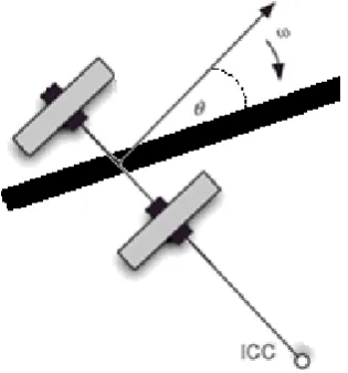
Deployment of the filtered algorithm in the rotary encoders needs a mathematical model in state matrix. The model should have as input the voltage signal that goes to the motors and as an output the angular velocity of the motor shaft, for later obtain an angular velocity desired in each motor. Infrared sensors measure the angular separation between the line of the track and the central front part of the robot, represented by ϴ (Fig. 5).

The software reads the value of each one of the infrared sensors. Based on it, a function returns a proportional number to the angle to measure. Representation of infrared sensors is in either analogue or digital. If it is in analogue, it samples at any speed and facilitate the management by the controller. The counterpart is that the measurement becomes very sensitive to any change in the environment illumination and will need an Analogue/Digital conversion process, turning the information acquisition in a slow process. If it is in digital, the sensors reading process run faster obtaining a more robust signal than the environmental noise, although the use of digital values makes less suitable the operation by the controller because of the introduction of a quantization error.

The implemented solution was to complement the sensors’ digital values with the angular velocity measured by the gyroscope. The union of both data results in an analogue signal managed by the controller.

2.2.4. Main controller

The main controller defines the spinning velocity of each wheel, i.e., fix the reference of the velocity controller in each motor, decision based in the angular position and the linear velocity the robot needs.

Fig. 5. Angular separation between the robot and the track.

2.2.5. Robot final design

Figure 6 depicts the feedback system for each motor. Block M(z) represents the motor´s transfer function that has as input the motor supply voltage and as output the motor angular velocity.

Interruption occurs at 0.5 ms on the program code. Between each interruption runs the filtered algorithm, having as input both the angular velocity measured by the encoders and the last PWM value sent to the motor. With these parameters, Kalman algorithm makes an estimation of the motor angular velocity. The reference value subtracts this value to obtain the signal error, and with this signal as input parameter, the controller runs. Based on the measured error, the controller decides the new PWM value and the loop continues until next interruption occurs. Each motor implements this system.

Fig. 6. Feedback system for motor velocity control.

Figure 7 depicts the transfer function with the reference value of the robot angular velocity as input, and the robot angular velocity as output. The Mr1 block represents the feedback system shown in Figure 6 for a motor and the Mr2

be similar to the entry value, as feedback system designed for this purpose.

The previous system is summarized in a block named H and represented with the feedback principal system in Figure 8, that depicts an useful system to control the robot angular position. In software, when an interruption of 1.5 ms happens, the filtered algorithm equations run as input parameter the gyroscope angular velocity readout and the angular position readout of the infrared sensors. The algorithm combines both data and makes an angular position estimation. The reference value subtracts this value to get the error signal that enters into the controller.

Fig. 7. Transfer function between the reference and real angular value of the robot.

Based on the error measured, the controller decides the new reference value for the H block. This block output depicts the robot angular velocity and the angular position (its integral). Next interruption measures these values again and the loop repeats.

Fig. 8. Feedback system for control of the angular position.

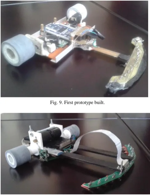
Carry out the project involved the construction of two models. Figure 9 depicts the first prototype built. For this design, the PCB was made of Bakelite, a not very resistant material, reason to add aluminium parts to hold the chassis. Besides, the motors were installed in each side of the robot, causing an increment of the inertial moment. Wheels of 2.1 cm of radius were necessary to reach a velocity of 2 m/s, due to the gears available had a relation of 8:1 and did not achieve a higher speed with a lesser radius.

gears to 48:10. Moreover, it was used the SolidWorks software to design the supports that hold the motors and rings where the robot’s wheels are placed.

Fig. 9. First prototype built.

Fig. 10. Final design of the robot.

III. RESULTS

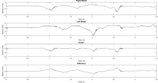
Figure 11 depicts the route of the robot in a competition racetrack, with a total longitude of 5.84 m, formed by curves and straight lines, ideal for testing. Figure 12 shows the results with four graphics. The first one depicts the right wheel velocity during the path. The second one depicts the velocity during the track of the left wheel. Both data obtained from the motor rotational encoders that correspond to the respective side. The third graph depicts the velocity at which the robot mass center moves along the path, that is the average of the dos previous measures. The last graph depicts the existing difference between velocities in both sides, base of the locomotion in this type of robot with differential configuration, being the measure of the robot’s angular velocity multiplied by a proportional constant.

Among principal results obtained, the total time the robot took its route was approximately 3.5 seconds, so the media velocity of the robot through the path is 1.67 m/s approximately. Finally, considering the sprinter robot mass centre, it reached its maximum velocity in straight lengths,

where its value is 2.23 m/s approximately. This velocity diminishes in curves.

It has to be considered these values are exclusive to the path followed and can vary depending on its course, thus constraints will be established according the curve with the lesser curvature radius possible, as well as the circumference arc angle that it has. Analysing these data, it is evident the sprinter robot reaches very good velocities for competitions.

Fig. 11. Sprinter robot test on the racetrack.

IV. CONCLUSIONS

The use of FPGA allows designing a microcontroller very optimally with integration of several modules in a single chip. With the use of the Kalman filter as a complement (for the signals read out from the rotary encoders) an improvement in the motor velocity control was experienced and allowed to combine the information obtained from the infrared sensors array and from the gyroscope to estimate the angular separation and its derived.

The cascade feedback allows stabilizing the robot position combining data of the wheels velocity and the angular position. Data acquisition allows analysing in detail the robot behaviour, whether algorithms related to control and filtering or implement strategies. MATLAB allows working in code improvements simulating the acquired data.

Fig. 12. Robot velocities during the circuit track.

REFERENCES

[1] H. I. V. Jadan, C. R. M. Vera, R. P. Intriago y V. S. Padilla, «Implementing a Kalman Filter on FPGA Embedded Processor for Speed Control of a DC Motor Using Low Resolution Incremental Encoders,» Lecture Notes in Engineering and Computer Science: Proceedings of the World Congress on Engineering and Computer Science 2016, vol. I, pp. 367-371, 2016.

[2] FAULHABER (2016), DC-Micromotors Precious Metal Commutation Series 2224…SR. EN_2224_SR_DFF.PDF. [Online]. Available: https://fmcc.faulhaber.com/resources/img/

[3] POLOLU (2013, Jul). TB6612FNG Dual Motor Driver Carrier. [Online]. Available: https://www.pololu.com/product/713

[4] POLOLU (2016, Oct). Pololu 5V, 5A Step-Down Voltage Regulator D24V50F5. [Online]. Available: https://www.pololu.com/product/2851

[5] POLOLU (2016, Oct). QTR-1A Reflectance Sensor. [Online]. Available: https://www.pololu.com/product/958

[6] POLOLU (2016, Oct). MinIMU-9 v3 Gyro, Accelerometer, and Compass (L3GD20H and LSM303D Carrier). [Online]. Available: https://www.pololu.com/product/2468

[7] Altera (2011, May). RS232 UART for Altera DE-Series Boards. RS232.pdf. [Online]. Available: ftp://ftp.altera.com/up/pub/Altera_Material/11.1/University_Program_I P_Cores/Communications/

[8] Altera (2011, May). NIOS II Hardware Development Tutorial. tt_nios2_hardware_tutorial.pdf. [Online]. Available: http://www.altera.com/literature/tt/