Implementation of the Curve Number Method and the KINFIL Model in the Smeda Catchment to Mitigate Overland Flow with the Use of Terraces

Implementation of the Curve Number Method

and the KINFIL Model in the Smeda Catchment

to Mitigate Overland Flow with the Use of Terraces

Pavel KOVÁŘ*, Darya FEDOROVA and Hana BAČINOVÁ

Department of Land Use and Improvement, Faculty of Environmental Sciences,

Czech University of Life Sciences Prague, Prague, Czech Republic

*Corresponding author: [email protected]

Abstract

Kovář P., Fedorova D., Bačinová H. (2018): Implementation of the curve number method and the KINFIL model in the Smeda Catchment to mitigate overland flow with the use of terraces. Soil & Water Res., 13: 98−107.

The Smeda catchment, where the Smeda Brook drains an area of about 26 km2_{, is located in northern}

Bohe-mia in the Jizerské hory Mts. This experimental mountain catchment with the Bily Potok downstream gauge profile was selected as a model area for simulating extreme rainfall-runoff processes, using the KINFIL model supplemented by the Curve Number (CN) method. The combination of methods applied here consists of two parts. The first part is an application of the CN theory, where CN is correlated with hydraulic conductivity K_s of the soil types, and also with storage suction factor S_f at field capacity FC: CN = f(K_s, S_f). The second part of the combined KINFIL/CN method, represented by the KINFIL model, is based on the kinematic wave method which, in combination with infiltration, mitigates the overland flow. This simulation was chosen as an alternative to an enormous amount of field measurements. The combination used here was shown to provide a successful method. However, practical application would require at least four sub-catchments, so that more terraces can be placed. The provision of effective measures will require more investment than is currently envisaged.

Keywords: CN method; infiltration; kinematic KINFIL model; wave

The discharges in the limnigraphic profile at the

outlet of the Bily Potok profile of the Smeda

catch-ment have been measured continuously since 1957.

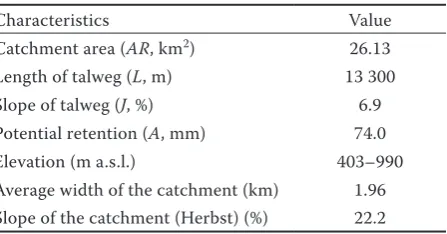
The physical and geometric characteristics of the

catchment are provided in Table 1. The catchment

area is 26.13 km

.

MATERIAL AND METHODS

Smeda catchment

.

Table 2 presents the

hydro-logical situation and the N-year discharges. Table 3

documents the calculation of the average value of the

Curve Number CN

= 77.5. This value is relatively

high, and indicates low infiltration capacity through

the hydrologic soil group C (77%). The remainder of

the soils belongs to the hydrologic group B, i.e. soils

with low sorptivity (oligo-mesotrophic soils, podzolic

peat-brown soils, and peaty-gley soils). The relative

substitution of the first granulometric category is

20% to 25%, and the coefficient of saturated hydraulic

conductivity

K

< 10 mm/h. The surface of the

for-ested part of the catchment (88%) can be classified

Characteristics Value Catchment area (AR, km2_{) 26.13}

under Forest Hydrological Conditions (FHC) = 2, on

the basis of the compactness of “forest litter” when

timber understorey (TU) = 1 (depth < 5 cm).

Since 1957, three rainfall observatories have been

installed: at Hejnice, at Nove Mesto and at Bily Potok.

All weighted rainfall means have also been measured,

together with their direct discharge flows to the

Smeda River at the Bily Potok catchment outlet. The

basic characteristics of the catchment were derived

from geographical maps, and are presented in

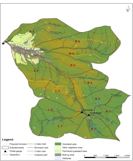
Fig-ure 1. For modelling rainfall – runoff, it is important

to obtain correct values of the curve numbers (CN)

(NRCS 2004a, b) as the starting values for the

pa-rameters of the model: hydraulic conductivities

K

,

and the sorptivity values at the field capacities

S

.

The values of CN are influenced by land use. In the

the Smeda catchment, the land is used mainly for

forestry.

Table 2. N-year discharges from the Bily Potok profile in the Smeda catchment, (source Czech Hydrometeorological Institute, data 2015)

Return period (N-years) 1 2 5 10 20 50 100 Discharges QN(m3/s) 21 33 54 74 97 132 162

Table 3. Curve Number (CN) for the Bily Potok profile in the Smeda catchment

Land use Area _(%) Hydrol soil _group CN Weighted _{mean CN}

Forest 70₁₈ C_B 79₆₉ 55.3_12.4

Pastures 7 C 79 5.5 Arable land 3 B 79 2.4 Urbanized area 2 – 98 1.9

Total 100 – – 77.5

Figure 1. Selected characteristics of the Smeda catchment

The Smeda catchment Elevation

Geology

Watershed divide Orthogneiss Granodiorite Metagranite granite

Wetlands (peat soils) Slope sediments Loam, Sand, Gravel

Slopes

Soils Land use

Watershed divide Modal Cambisols Cambisols Gleysols Podzols Organosols

Outlet profile Watershed divide Smeda river Tributaries Wetlands Forest Grassland Other green areas Urbanised area max. 1148 m a.s.l.

min. 371 m a.s.l. Sub-catchment Contourline Watershed divide

max. 100%

In addition, we optimized the design of the terraces for

the simplest one-route, or three-routes, or five-routes

in parallel. For this task, just four sub-catchments were

selected. Sub-catchments R5, R6, and L3, L4 were

de-signed. Unfortunately, the water discharges of the four

sub-catchments (R5, R6 and L3, L4) in urbanized areas

of the village of Bily Potok reach high values, despite

the five rows of terraces (Figure 2).

Table 4 provides the parameters of standard flood

control terraces, when they are 10.0 m in width and

the central part is 5.0 to 7.0 m in length, with a slight

slope of 0.01 to 0.03. The total sum of the lengths

of all the terraces is 6488 m. Figure 3 presents the

transversal profile of the terraces. It shows the

com-parability between filling and excavated parts of the

natural soil material.

Computations without the design of biotechnical

measures were applied with short torrential rainfalls

for a return period of

N

= 2, 10, and 100 years, and

40 min and 60 min in duration (Table 4), i.e. the

conditions for which the critical culmination of the

discharges was computed (

N

= 2 years is not printed

here). The time translation of the runoff is dependent

on travelling time

T

, which can be computed using

the US SCS methodology (US SCS 1986, 1992), or

according to Ferguson (1998), as follows:

T

= (3.28 ×

L

)0.8/1900 ×

J

(1)

where:

L – hydraulic length of the thalweg (m) J₀ – slope of the thalweg (%)

For CN = 77.5 the potential retention of the catchment A is 74.0 mm.

Natural gravel-bed channels are composed of

hetero-geneous sized grains at different spatial scales. Mao

and Surian (2010) investigated sediment mobility

and demonstrated the relationships between shear

stress and sediment transform (Laronne & Shlomi

2007; Chang & Chung 2012). An alternative method

that has been recently developed in image processing

techniques has shown promising as a viable method

for measuring gravel and larger size fluvial sediment

(Beggan & Hamilton 2010). Hallema and Moussa

(2014) used a distributed model for overland flow and

channel flow based on a geomorphologic

Terrace

(n) Sub-catchment (n)

Length Entire length Width Slope

(–) Roughness – Manning n (–) (m)

5 R5 1794 1794 10.0 0.01 0.150

6 + 7 R6 684 + 1468 2152 10.0 0.01 0.150

3 + 4 L3 821 + 696 1517 10.0 0.01 0.150

1 + 2 L4 391 + 634 1025 10.0 0.01 0.150

Sum of lengths = 6488 m

Figure 2. Design of the orderlines of each of the terraces in the Smeda catchment, sub-catchments R5, R6, L3 and L4

Figure 3. Transversal profile of the terraces designed for the Smeda catchment

FILLING

EXCAVATED _ORIGINA

L TE RRAIN

ous unit hydrograph (GIUH) method. Quantification

of the size distribution of fluvial gravels is an

impor-tant issue in the studies of river channel behaviour

in hydraulics, hydrology and geomorphology. For all

the computations, we used our own DES_RAIN

soft-ware (Vaššová & Kovář 2012), which is available on

http://fzp.czu.cz/vyzkum/. Table 5 provides the design

rainfall depths

P

(mm) and the duration in minutes.

Combining the Curve Number method and the

KINFIL model

. A combination of the CN method

and the KINFIL model (Kovar 1989, 2014) provides

a schematic representation of the Smeda catchment

data for the KINFIL model (Tables 6 and 7).

The current version of the KINFIL model is based

on the Green-Ampt infiltration theory, with

pond-ing time accordpond-ing to Mein and Larson (1973) and

Morel-Seytoux (Morel-Seytoux & Verdin 1981;

Morel-Seytoux 1982; Ponce & Hawkins 1996):

for the Bily Potok observatory

N (years) Rainfall duration (t, min)

24 h 20' 40' 60' 120' 2 66.8 27.16 32.74 35.47 40.70 5 95.0 41.37 52.07 56.40 64.65 10 113.1 51.67 65.50 70.94 81.24 20 132.0 64.04 81.90 88.71 101.52 50 155.1 79.82 103.61 112.23 128.82 100 173.2 92.15 120.00 129.98 148.91

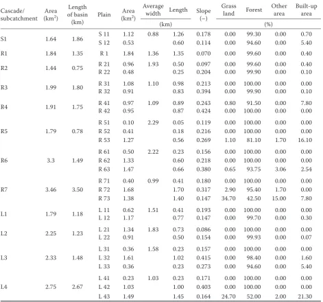
Table 6. Scheme of the Smeda catchment for the KINFIL model

Cascade/

subcatchment (kmArea 2₎

Length of basin

(km) Plain

Area (km2₎

Average

width Length Slope (–)

Grass

land Forest Other area Built-up area

(km) (%)

S1 1.64 1.86 _{S 12}S 11 1.12_0.53 0.88 1.26_0.60 0.178_0.114 0.00_{0.00 94.60}99.30 _0.000.00 0.70_5.40

R1 1.84 1.35 R 1 1.84 1.36 1.35 0.070 0.00 99.60 0.00 0.40

R2 1.44 0.75 _{R 22}R 21 0.96_0.48 1.93 0.50_0.25 0.097_0.204 0.00_{0.00 99.90}99.60 _0.000.00 0.40_0.10

R3 1.99 1.80 R 31_{R 32} 1.08_0.91 1.10 0.98_0.83 0.213_0.394 0.00 100.00_{0.00 99.90 0.00}0.00 0.00_0.10

R4 1.91 1.75 R 41_{R 42} 0.97_0.95 1.09 _0.870.89 0.243_0.424 0.80_{0.00 100.00}91.50 _0.000.00 7.80_0.00

R5 1.79 0.78

R 51 0.10 2.29 0.05 0.119 0.00 100.00 0.00 0.00 R 52 0.41 0.18 0.216 0.00 100.00 0.00 0.00 R 53 1.27 0.56 0.269 1.10 81.10 1.70 16.10

R6 3.3 1.49

R 61 0.50 2.22 0.23 0.156 0.00 100.00 0.00 0.00 R 62 1.33 0.60 0.218 0.00 100.00 0.00 0.00 R 63 1.47 0.66 0.380 0.65 93.75 3.06 2.54

R7 3.46 3.50

R 71 0.40 0.99 0.41 0.180 0.00 100.00 0.00 0.00 R 72 1.68 1.70 0.317 2.90 95.40 1.70 0.00 R 73 1.38 1.40 0.147 34.70 42.50 15.00 7.80

L1 1.79 1.18 L 11_{L 12} 0.62_1.17 1.51 0.41_0.77 0.193_0.147 0.00 100.00_{0.00 99.70 0.00}0.00 0.00_0.30

L2 2.25 1.23 L 21_{L 22} 1.34_0.91 1.83 0.73_0.50 0.086_0.154 0.00 100.00_{0.00 99.93 0.00}0.00 0.00_0.07

L3 2.33 1.48

L 31 0.36 1.58 0.23 0.157 0.00 100.00 0.00 0.00 L 32 1.61 1.02 0.415 0.00 98.40 0.00 1.60 L 33 0.36 0.23 0.273 0.00 94.60 0.00 5.40

L4 2.75 2.67

K

(

z

+

H

/

z

) = (θ

– θ

)

dz

/

dt

(2)

S

= (θ

– θ

) ×

H

(3)

t

=

S

/

i

× (

i

/

K

– 1)

(4)

K_s – hydraulic conductivity (m/s)

z_f – the vertical extent of the saturated zone (m) θ_s – water content at natural saturation (–) θ_i – initial water content (–)

H_f – wetting front suction (m) I – rainfall intensity (m/s) S_f – storage suction factor (m) t_p – ponding time (s)

t – time (s)

The main task is to assess hydraulic

conductiv-ity 

K

, and the storage suction factor

S

(at field

ca-pacity, 

FC

)

.

These

two parameters can be measured

directly on small experimental catchments. In larger

catchments, the previously derived relationships of

these parameters and the CN, which are widely used

by Soil Conservation Service (SCS) (US SCS 1986),

can also be applied. The CN correspond with the

conceptual values of soil parameters

K

and

S

(

FC

):

CN =

f

(

K

,

S

)

.

The CN method, developed by the US Soil

Con-servation Service based on soil types (Brakensiek

& Rawls 1981), design rainfall depths and duration,

vegetation cover, land use, and antecedent moisture

conditions, is widely used due to its easy application.

An evident shortcoming of this methodology is that

it disregards both the intensity and the duration of

the rainfall that causes flood runoff. This

imperfec-tion can be dealt with by using the physically-based

infiltration approach of the KINFIL model (Kovář

1992) instead of the usual empirical CN approach.

The relationships between the CN method and the

soil type parameters have been used for the

infiltra-tion process. These relainfiltra-tionships were derived by

correlating the data from 62 gauges located in the

Czech territory (Šamaj

et al

. 1983; Kovář 1992) and

the parameters of the basic soil groups.

RESULTS AND DISCUSSION

The computed CN values for the Smeda catchment

are shown in Table 8.

Table 9 shows the principles for computing the

results from the correlation processes to change the

hydraulic conductivity

K

(mm/h) and the sorptivity

S

(θ

) (mm/h

at field capacity). When this

sorptiv-ity

S

(θ

) is amended to the storage suction factor,

its form can be expressed as follows:

S

= (

S

(θ

)

/2.0 ×

K

s

)

(5)

The second part of the KINFIL model simulates

the propagation and the transformation of the direct

runoff (Beven 2006). The partial differential

equa-tion describes the unsteady flow approximated by

a kinematic wave on a cascade of planes arranged

according to the topography of the catchment:

(6)

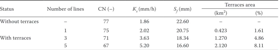
Table 7. Correlation relationships CN = f (K_s, S_f), orderlines of the terraced area

Status Number of lines CN (–) K_s (mm/h) S_f (mm) Terraces area (km2_{) (%)}

Without terraces – 77 1.86 22.60 – –

With terraces

1 75 2.02 20.75 0.423 1.61

3 71 3.63 18.34 1.270 4.86

5 67 5.20 16.60 2.120 8.11

CN – Curve Number; Ks – hydraulic conductivity; Sf – storage suction factor

Table 8. Curve Number (CN) values derived from the Smeda catchment for the soil types (US classification and Czech Bily Potok major profile)

Soil types

1 2 3 4 5 6 7 8 9 10

CN 95.1 92.1 90.0 86.8 85.8 78.0 64.1 60.7

US soil types (Brakensiek and Rawls (1981), amended by the Czech soil classification according to Novak)

 

α m

e

y _my y _{i t}

t x



 _{ } _

where:

x, y, t – length (m), depth (m) and time (s) α, m – hydraulic parameters

i_e(t) – excess rainfall intensity (m/s)

This equation is solved by the finite difference

method, using an explicit numerical scheme.

N

umeri-cal stability of the scheme is ensured if the time and

space step is according to equation (7):

(7)

where: c – celerity c = m × ym–1

y – water depth

Explicit schemes in the software where there is only

one unknown on the left-hand side of the equation

are quick, but they are sensitive to the stability of

the computation, if there is a bigger difference in the

time (Δ

t

) and space step (Δ

x

) (Eq. (7)).

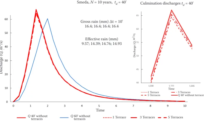
To ensure safe biotechnical measures, it is

neces-sary to construct multiple terraces in a contour line

system. In the Smeda basin, one row 10 m in width

has been built in four sub-catchments R5, R6, and

L3, L4. For a greater level of safety, the Bily Potok

municipality will need at least five rows of terraces to

decrease the water discharges for

N

= 10-year flood

from 67.0 m

/s (without terraces) to about 64.5 m

/s.

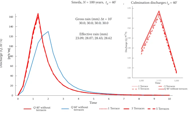
The Tables 10−13 and Figures 4 and 5 provide results

that reduce the cumulation of

N

=100-year discharges

from 167.3 m

/s (without terraces) to about 162.0 m

/s.

The most dangerous time situation is duration of

40 min. A similar computation was also performed

for a torrential rain of 60 min in duration, but this is

a less dangerous scenario.

Table 9. Instruction from the correlation processes for hydraulic conductivity K_s (mm/h) and storage suction factor S_f (mm)

Conditions for CN Equation Accuracy(σ)

K_s equations (mm/h)

if CN ≥ 75 0.084

if 74 ≥ CN < 36 K_s = 31.4 – (0.39 × CN) 0.136 if CN < 35 K_s = 47.1 – (0.82 × CN)

S(θFC) equations (mm/h0.5)

if CN > 65

if CN < 64 S(θFC) = 30.25 – (0.15 × CN)

CN – Curve Number; S_f = S(θ_FC)2_{/2.0 × K}

s

100 CN 12 4

S

K  



 

FC

S  

1

t c

x

 _



Figure 4. Smeda, N = 10 years, time duration t_d = 40 min; discharges without terraces, 1 terrace, 3 terraces, 5 terraces

Culmination discharges t_d = 40' Smeda, N = 10 years, t_d = 40'

Gross rain (mm) Δt = 10' 16.4; 16.4; 16.4; 16.4

Effective rain (mm) 9.57; 14.39; 14.76; 14.93

Di

sc

har

ge (

Q

,

m

3/s)

Time 1 Terrace

5 Terraces 3 TerracesQ 40' without terraces

Time

Di

sc

har

ge (

Q

, m

3/s)

Q 40' without

Figure 5. Smeda, N = 100 years, time duration t_d = 40 min; discharges without terraces, 1 terrace, 3 terraces, 5 terraces Table 10. Maximum N = 10 years and N = 100 years discharges (Q, m3_{/s) with duration of 40 min, without terraces and}

with 5 rows of terraces

Seq. Time _(h)

10 years 100 years

Seq. Time _(h)

10 years 100 years without

terraces 5 rows of terraces without terraces 5 rows of terraces without terraces 5 rows of terraces terraceswithout 5 rows of terraces 1 0.333 4.461 4.252 19.226 17.906 16 5.333 3.164 3.149 3.368 3.353 2 0.666 20.023 18.913 69.224 64.570 17 5.666 2.643 2.631 2.789 2.776 3 1.000 42.347 40.005 129.138 123.765 18 6.000 2.235 2.225 2.339 2.329 4 1.333 67.069 64.454 167.356 161.927 19 6.333 1.909 1.900 1.983 1.974 5 1.666 53.926 52.618 105.956 103.828 20 6.666 1.644 1.637 1.698 1.690 6 2.000 38.737 38.091 67.480 66.622 21 7.000 1.427 1.421 1.466 1.460 7 2.333 27.635 27.296 44.925 44.524 22 7.333 1.248 1.242 1.275 1.269 8 2.666 20.400 20.205 30.333 30.117 23 7.666 1.097 1.092 1.117 1.112 9 3.000 15.540 15.419 20.845 20.715 24 8.000 0.970 0.966 0.985 0.981 10 3.333 12.181 12.101 14.843 14.759 25 8.333 0.862 0.858 0.874 0.870 11 3.666 9.580 9.524 10.963 10.905 26 8.666 0.769 0.766 0.779 0.776 12 4.000 7.507 7.466 8.332 8.290 27 9.000 0.690 0.687 0.699 0.696 13 4.333 5.920 5.889 6.476 6.444 28 9.333 0.622 0.619 0.629 0.626 14 4.666 4.735 4.711 5.127 5.103 29 9.666 0.563 0.561 0.569 0.567 15 5.000 3.843 3.824 4.125 4.106 30 10.000 0.512 0.510 0.517 0.515 Seq. − sequence

Table 11. Effectiveness of the terraces in the Smeda catchment, N = 10 and 100 years, time duration t_d = 40 and 60 min (effective rainfall; 5 rows of terraces)

Without terraces With terraces Without terraces With terraces

N = 10, t_d = 40': RER = 56.7 mm RER_T = 55.9 mm N = 100, t_d = 40': RER = 112.2 mm RER_T = 110.4 mm

N = 10, td = 60': RER = 59.7 mm RER_T = 58.7 mm N = 100, td = 60': RER = 118.8 mm RER_T = 117.8 mm

RER – effective rainfall without terraces (mm); RER_T – effective rainfall with terraces (mm)

Culmination discharges t_d = 40' Smeda, N = 100 years, t_d = 40'

Gross rain (mm) Δt = 10' 30.0; 30.0; 30.0; 30.0

Effective rain (mm) 23.09; 28.07; 28.43; 28.62

Di

sc

har

ge (

Q

,

m

3/s)

Time 1 Terrace

5 Terraces 3 TerracesQ 40' without terraces

Time

Di

sc

har

ge (

Q

, m

3/s)

Q 40' without

For a comparison with the

N

-year discharges on

the Smeda catchment, we computed Tables and

Fig-ures with geometric factors for sub-catchments and

their land use. The same procedure was followed,

in principle, for

N

= 2 years and 40 min duration.

However, this computation is not presented here.

CONCLUSION

Slope terraces have hydro-physical

characteris-tics that can be different and they require a lot of

finances. Hydrological analyses indicate that the use

of flood control terraces as biotechnical measures

does not provide any effective barriers for the Bily

Potok municipality. For a practical application, more

than four sub-catchments are needed. In addition,

more than five rows of terraces are needed, and also

at least two polders. The provision of effective

meas-ures will require more investment than is currently

envisaged. A comparison of the computational results

(Table 10) shows that correct results are dependent

on regular maintenance.

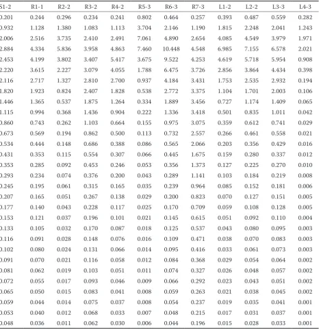
Table 12. Discharges (Q, m3_{/s) from individual sub-catchments of the Smeda catchment, N = 10 years, time duration 40 min}

Acknowledgements. Supported by Project N TA02020402 of Technological Agency of the Czech Republic and by the In-ternal Grant Agency of the Faculty of Environmental Sciences as a part of the Project IGA2017 20174257 – Modelling of the overland flow to mitigate harmful impact of soil erosion.. The team of authors express their gratitude for this support.

References

Beggan C., Hamilton C.W. (2010): New image processing software for analysing object size-frequency distribution,

geometry, orientation, and spatial distribution. Comput-ers & Geosciences, 36: 539–549.

Beven K.J. (2006): Rainfall-Runoff Modelling. The Primer. Chichester, John Wiley & Sons.

Brakensiek D.L., Rawls W.J. (1981): An infiltration based rainfall-runoff model for a SCS type II distribution. In: Winter Meeting ASAE. Palmer House, Chicago. Chang F.J., Chung C.H. (2012): Estimation of riverbed

grain-size distribution using image-processing techniques. Journal of Hydrology, 440–441: 102–112.

Ferguson B.K. (1998): Introduction to Stormwater. New York, J.Wiley & Sons, Inc.

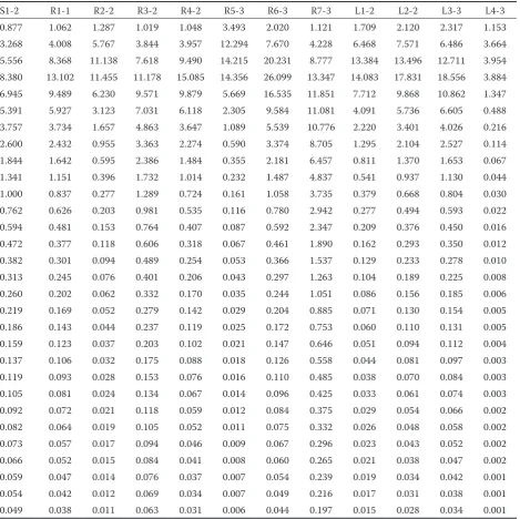
Table 13. Discharges (Q, m3_{/s) from individual sub-catchments of the Smeda catchment, N = 100 years, time duration}

40 min

Hallema D.W., Moussa R. (2014): A model for distributed GIUH-based flow routing on natural and anthropogenic hillslopes. Hydrological Processes, 28: 4877–4895. Kovář P. (1989): Rainfall-runoff Event Model Using Curve

Numbers (KINFIL). Research Report No. 110.92. Wa-geningen, Department of Hydraulics and Catchment Hydrology.

Kovář P. (1992): Possibilities of determining design dis-charges on small catchments using KINFIL model. Vodohospodářsky časopis (Water Resources Journal), 40: 197–220.

Kovář P. (2014): KINFIL Model: Infiltration and Kinematic Wave. User’s Manual. Prague, FZP CZU.

Laronne J.B., Shlomi Y. (2007): Depositional character and preservation potential of course-grained sediments de-posited by flood events in hyper-arid braided channels in the Rift Valley, Arava, Israel. Sedimentary Geology, 195: 21–37.

Mao L., Surian N. (2010): Observations on sediment mo-bility in a large gravel-bed river. Geomorphology, 114: 326–337.

Mein R.G., Larson C.L. (1973): Modelling infiltration dur-ing a steady rain. Water Resources Research, 9: 384–394. Morel-Seytoux H.J. (1982): Analytical results for prediction

of variable rainfall infiltration. Journal of Hydrology, 59: 209–230.

Morel-Seytoux H.J., Verdin J.P. (1981): Extension of the SCS Rainfall Runoff Methodology for Ungaged Watersheds. [Report FHWA/RD-81/060.] Springfield, US National Technical Information Service.

NRCS (2004a): Hydrologic soil-cover complexes. Chapter 9. In: National Engineering Handbook, Part 630 Hydrology. Washington D.C., USDA.

NRCS (2004b): Estimation of direct runoff from storm rainfall. Chapter 10. In: National Engineering Handbook, Part 630 Hydrology. , Washington D.C, USDA.

Ponce V.M., Hawkins R.H. (1996): Runoff Curve Number: Has it reached maturity? Journal of Hydrologic Engineer-ing, 1: 11–19.

Šamaj F., Brázdil R., Valovič J. (1983): Daily depths of ex-treme rainfalls in 1901–1980 in CSSR. In: Study Proceed-ings of SHMU. Bratislava, ALFA: 19–112. (in Czech and Slovak)

US SCS (1986): Urban Hydrology for Small Watersheds. Technical Release 55 (updated). US Soil Conservation Service.

US SCS (1992): Soil Conservation Program Methodology. Chapter 6.12. Runoff Curve Numbers. US Soil Conserva-tion Service.

Vaššová D., Kovář P. (2012): DES_RAIN, Computational Program. Prague, FZP CZU.