A Panel Cointegration Analysis of the Exchange Rate Pass Through

Munich Personal RePEc Archive

A Panel Cointegration Analysis of the

Exchange Rate Pass-Through

Ben Cheikh, Nidhaleddine and Mohamed Cheik, Hamidou

ESC Rennes School of Business, International University of Rabat,

Central Bank of the Comoros

September 2013

Online at

https://mpra.ub.uni-muenchen.de/50123/

A Panel Cointegration Analysis

of the Exchange Rate Pass-Through

Nidhaleddine Ben Cheikh

and Hamidou Mohamed Cheik

a_{ESC Rennes School of Business, Rue Robert d’Arbrissel, 35065, Rennes, France}

b_{International University of Rabat, Technopolis Rabat-Shore, 11100, Rabat, Morocco}

c_{Central Bank of the Comoros, Place de France, BP 405, Moroni, Comoros}

Abstract

This paper investigates the presence of a long-run equilibrium relationship in the exchange rate pass-through (ERPT) equation for a panel of 27 OECD countries. Previous empirical panel data studies, such as BARHOUMI(2005), have neglected

the possibility of cross-sectional correlation and spillovers amongst countries. Since the strong economic and financial linkages between OECD countries cannot be ignored, we apply second generation panel unit root and panel cointegration tests which account for possible cross-section dependence across the units in the panel. Our results suggest the existence of a cointegrated equilibrium relationship between the variables in levels, as implied by the theoretical underpinning of the ERPT mechanism. When estimating the long-run pass-through coefficient, both FM-OLS and DOLS estimators show an incomplete pass-through, i.e. import prices sensitivity to exchange rate movements does not exceed 0.70% for our sample of OECD countries. This evidence of partial pass-through would represent a key element in understanding the ongoing global external imbalances.

J.E.L classification: C23, F31, F40

Keywords: Exchange Rate Pass-Through, Import Prices, Non-stationary Panels

1

Introduction

The concept of the exchange rate pass-through (ERPT) refers to the degree of sensitivity of import prices to a one percent change in exchange rates in the importing nation’s currency. Thorough knowledge of the degree of pass-through is of particular importance for several policy issues, including the design of monetary policy, adjustment in trade balances, the international transmission of shocks and the optimal choice of exchange rate regime. As import prices are a principal channel through which movements in the exchange rate affect domestic prices and hence also the variability of inflation and output, these considerations would ultimately have important implications for the appropriate stance of monetary policy. If the inflationary effects of exchange rate changes are large, the central bankers will have to implement monetary policies that could offset the inflationary consequences of exchange rate changes. Policymakers must be able to gauge how large these effects are likely to be, in order to determine the size and persistence of underlying inflation pressures and any monetary policy responses that might be required to deal with them.

In a comprehensive survey of the ERPT literature, MENON(1995) summarized

the results of 43 papers and revealed some shortcomings of previous empirical pass-through studies. More specifically, time-series properties of the data, particularly the non-stationarity and cointegration in the data, are not properly taken into account. Failed to find evidence in the data for cointegration, several studies has estimated ERPT models in first differences where the information contained in "levels" variables is lost. Nevertheless, as predicted by the theoretical underpinning of the ERPT mechanism, a long-run or steady-state relationship between the levels of the key variables, i.e. exchange rate and price series, should exist. Thus, using appropriate estimation techniques would help restore a cointegrated equilibrium relationship between the variables in levels. Recently, there has been an increasing use of unit root and cointegration analysis in the context of panel data. As discussed in panel cointegration literature (see e.g. PEDRONI, 1999, 2001, 2004; BREITUNG

and PESARAN, 2005, among others), conventional nonstationary tests have low power in small sample sizes, so adding the cross-section dimension to the time series dimension would increase the power of these tests.

Thus, due to recent developments in time series and panel data econometrics, some studies of pass-through explicitly recognize the fact that exchange rate and price series are often non-stationary and may be cointegrated, although the number of those empirical works is still sparse. For example, in a panel of 24 developing countries, BARHOUMI(2005, 2006) gives support to the presence of a long-run

equilibrium relationship between variables entering the ERPT equation. The author employed the popular first generation tests for non-stationary panel data: the IM

tests for panel cointegration developed by PEDRONI(1999, 2004). Using the same approach, HOLMES(2006) were able to find a strong evidence of cointegrating

relationship consistent with the theoretical prediction of a steady state in the ERPT mechanism for 12 European Union countries. However, first generation tests, despite their advantages, are not exempt from critics. The key drawback of these tests is that the possibility of cross-sectional correlation and spillovers amongst countries are neglected. Indeed, the assumption of independence is usually is unrealistic, in particular in the analysis of macroeconomic or financial data which reveal strong inter-economy linkages.1 Then, it is very restrictive to assume that some countries, such as European Union or OECD members, are independent and no economic or financial linkage does exist between them. From econometric point of view, PESARAN(2007) argued that not accounting for possible cross-sections

dependence across units would entail a considerable size distortions in panels and may lead to flawed inference on the existence of the long-run relationship.

The goal of our paper is to overcome this mis-performance of first generation tests in the context of ERPT. We employ a class of panel unit root and panel cointegration tests which allow for serial correlation between the cross-sections, i.e. the so-called second generation tests. To the best of our knowledge, only

DE BANDT, BANERJEE, and KOZLUK (2008) have applied these recent panel

data techniques when investigating the issue of pass-through. In a sectoral study for 11 euro area countries, these authors show that the long-run relationship can be restored once appropriate panel econometric techniques are employed. Nevertheless, in our study, unlikeDEBANDT, BANERJEE, and KOZLUK(2008),

we consider larger and more heterogeneous sample of countries, namely 27 OECD countries. The existence of strong inter-economic linkages between OECD countries cannot plausibly be ignored. Consequently, we apply recently developed non-stationary panel techniques to tackle these issues. Also, we deal with the ERPT from a macroeconomic perspective using aggregate price measures, an issue of key importance for the conduct of monetary policy. Furthermore, second generation tests used in the context of our paper are different fromDE BANDT, BANERJEE,

and KOZLUK (2008). We employ the cross-sectionally augmented IPS panel unit root tests by PESARAN(2007) and the error-correction-based tests for panel cointegration by WESTERLUND(2007), which both account for possible

cross-sectional dependencies among the units included in the panel. To our knowledge, no other study has applied these non-stationary panel methods in the context of ERPT. Finally, in order to provide valid and reliable long-run ERPT coefficients, we apply both FMOLS and DOLS group mean estimators, as introduced by PEDRONI(2001), to estimate the long-run ERPT. This approach is quite relevant since it allows the

long-run cointegration relationships to be heterogeneous across countries. In other words, the advantage of these estimators is that they provide consistent estimates of the average cointegration slopes even if the slopes are in fact different across countries.

The remainder of this paper is organized as follows. Section 2 describes the analytical framework that underlies our empirical specification and the data used in the study. In Section 3, we discuss the empirical methodology used to test stationarity and cointegration in panel data. Both FM-OLS and DOLS estimators of the long-run ERPT are presented in Section 4. Section 5 concludes.

2

Analytical framework and Data description

2.1 Pass-Through Equation

Our approach is to use the standard specification used in the pass-through literature as a starting point (see e.g. GOLDBERG and KNETTER, 1997; CAMPA and

GOLDBERG, 2005). By definition, the import prices, MPit, for any country i

are a transformation of the export prices,X Pit, of that country’s trading partners,

using the nominal exchange rate,Eit (domestic currency per unit foreign currency):

MPit=Eit.X Pit (1)

Using lowercase letters to reflect logarithms, we rewrite equation (1)

mpit =eit+xpit (2)

where the export price consists of the exporters marginal cost,MCit and a markup,

MKU Pit

X Pit=MCit.MKU Pit (3)

In logarithms we have

xpit=mcit+mkupit (4)

So we can rewrite equation (2) as

mpit =eit+mcit+mkupit (5)

Markup is assumed to have two components: (i) a specific industry component and (ii) a reaction to exchange rate movements

Exporter marginal costs are a function of the destination market demand conditions,yit, and wages in exporting country,w∗_it:

mcit =η0yit+η1w∗it (7)

Substituting (6) and (7) into (5), we derive

mpit =αi+ (1+Φ)

| {z }

β

eit+η0yit+η1w∗it, (8)

The structure assumes unity translation of exchange rate movements. This empirical setup permits the exchange rate pass-through, represented byβ= (1+Φ), to depend on the structure of competition in one industry. Exporters of a given product can decide to absorb some of the exchange rate variations instead of passing them through to the price in the importing country currency. So ifΦ=0, the pass-through is complete and their markups will not respond to fluctuations of the exchange rates. This is the case when import prices are determined in the exporter’s currency (producer-currency pricing or PCP). And ifΦ=−1, exporters decide not to vary the prices in the destination country currency, thus they fully absorb the fluctuations in exchange rates in their own markups (LCP is prevailing).

Thus the final equation can be re-written as follows

mpit =αi+βeit+γyit+δw∗it+εit, (9)

The most prevalent result is an intermediate case where ERPT is incomplete (but different from zero), resulting from a combination of LCP and PCP in the economy. So, there is a fraction of import prices are set in domestic currency, while the remaining prices are set in foreign currency. Thus, the extent to which exchange rate movements are passed-through to prices will depend on the predominance of LCP or PCP: the higher the LCP, the lower the ERPT, and the higher PCP, the higher ERPT.

2.2 Data description

In this study, we consider the following panel of 27 OECD countries: Australia, Austria, Belgium, Canada, Czech Republic, Denmark, Finland, France, Germany, Greece, Iceland, Ireland, Italy, Japan, Korea, Luxembourg, Netherlands, Norway, New Zealand, Poland, Portugal, Slovak Republic, Spain, Sweden, Switzerland, United Kingdom and United States. The data are quarterly and span the period 1994:1-2010:4. Concerning our dependent variable, i.e. the domestic import prices,

mpit, we use the price of non-commodity imports of goods and services from

goods by excluding primary raw commodities because of their marked volatility.2 From the same database we take the real GDP as proxy for the domestic demand,

yit. To capture changes in foreign costs, we construct a typical export partners cost

proxy,W_t∗, that used throughout the ERPT literature (see e.g. BAILLIUand FUJII, 2004; CAMPA and GOLDBERG, 2005): W_t∗=Qt×Wt/Et, where Qt is the unit

labor cost based-real effective exchange rate,Wit is the domestic unit labor cost

and Et is the nominal effective exchange rate.3 Taking the logarithm we obtain

the following expression: w∗_it =qt+wt−et. Since the nominal and real effective

exchange rate series are trade weighted, we obtain a measure of foreign firms’ costs with each partner weighted by its importance in the domestic country’s trade. Data used to construct foreign producers costs - nominal effective exchange rate, consumer prices index and real effective exchange rate - are obtained from IMF’s International Financial Statistics.

3

Empirical tests

3.1 Panel unit root tests

Before testing for a cointegrating relationship, we investigate panel non-stationarity of the variables included in equation (9). Previous ERPT studies, such as

BARHOUMI(2005, 2006) and HOLMES(2006, 2008), has employed first generation

panel unit root tests whose main limit is the assumption of cross-sectional independence across units. More specifically, they used the t-bar test proposed by IMet al. (2003), which tests the null hypothesis of non stationarity. This test

allows for residual serial correlation and heterogeneity of the dynamics and error variances across groups. Thet-bar statistic is constructed as a mean of individual Augmented Dickey-Fuller (ADF) statistics and is designed to test the null that all individual units have unit roots. Nevertheless, it is very important to consider for the possibility of cross-sectional correlation and spillovers amongst countries. The hypothesis of no dependence across the panel members seems to be unrealistic regarding the economic and financial linkages prevailing in the OECD countries.4

2 _{As explained by IHRIG, MARAZZI, and ROTHENBERG(2006), when it was not possible to find} import prices of core goods that exclude all primary raw commodities, the inclusion of commodity prices indexes, such as oil prices, as independent variables should mitigate some of the noise generated by these volatile components.

3 _{The nominal effective exchange rate is defined as domestic currency units per unit of foreign} currencies, which implies that an increase represents a depreciation for home country.

To deal with this issue, we propose to use the cross-sectionally augmented IPS (CIPS) test as developed by PESARAN (2007). The author suggests a test for

cross-sectional dependence and offers a way of eliminating it by augmenting the usual ADF regression with lagged cross-sectional mean and its first-difference to capture the cross-sectional dependence that arises through a single-factor model.

PESARAN(2007) consider the following simple dynamic linear heterogeneous

panel data model:

yit = (1−ρi)µi+ρiyi,t−1+uit, i=1, . . . ,N; t =1, . . . ,T (10)

where the error termuit follow a single common-factor structure

uit =γift+eit, (11)

where ftis an unobserved common factor,γiis the corresponding factor loading

andeit is an idiosyncratic error term independent acrossiand independent of the

common factor. It is convenient to re-write (10) as

∆yit =αi+βiyi,t−1+γift+eit, (12)

where αi = (1−ρi)µi, βi =−(1−ρi) and ∆yit =yit −yi,t−1. The unit root hypothesis of interest,ρi=1, can now be expressed as

H0: βi=0, ∀i

against the possibly heterogeneous alternatives

H1:

βi<0 fori=1,2, ...,N1

βi=0 fori=N1+1,N1+2, ...,N

with 0<N1≤N

To account for the cross-sectional dependence induced by the common factor,

PESARAN(2007) suggest to cross-sectionally augment the test equation (12) with

sectional averages of the first differences and the lagged levels. The cross-sectionally augmented Dickey-Fuller regression is then given by

∆yit =ai+biyi,t−1+ciyt−1+di∆yt+εit, (13)

where y_t−1 = ∑Ni=1yi,t−1, ∆yt =∑Ni=1∆yit and εit is the regression error. The individual specific test statistic for the hypothesis H0i : βi=0 for a given i is

now thet-statistic ofbiin (13). The statistic is called cross-sectionally augmented

Dickey-Fuller (CADFi). The panel unit root for the hypothesis H0 : βi=0 for

cross-sectional average of theCADFitests, such that

CIPS= 1

N

N

∑

i=1

CADFi (14)

It is called CIPS, since it resembles the IPS statistic (IM et al., 2003). The critical values for the test statistics based on stochastic simulations are provided

in PESARAN(2007). Panel unit root tests results are shown in Table 1, for both

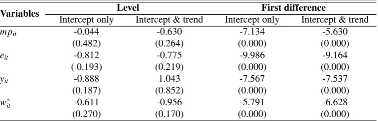
levels and first differences and with two specifications of the deterministics, namely with an intercept only and with an intercept and a linear trend. We use the Akaike information criterion to choose the appropriate lag-length. In the level case, we are unable to reject the null hypothesis that all series are non-stationary in favor of the alternative hypothesis that at least one series from the panel is stationary. For tests on the first differences, we can see that the null of non-stationarity is strongly rejected for all variables belonging to the pass-through equation. We thus conclude that all variables are stationary in first difference.5

Table 1:PESARAN’s (2007) test for panel unit root

Variables Level First difference

Intercept only Intercept & trend Intercept only Intercept & trend

mpit -0.044 -0.630 -7.134 -5.630

(0.482) (0.264) (0.000) (0.000)

eit -0.812 -0.775 -9.986 -9.164

( 0.193) (0.219) (0.000) (0.000)

yit -0.888 1.043 -7.567 -7.537

(0.187) (0.852) (0.000) (0.000)

w∗_it -0.611 -0.956 -5.791 -6.628

(0.270) (0.170) (0.000) (0.000)

Note:p-values for the null hypothesis of non stationarity are reported between parentheses. Individual lag lengths are based on Akaike Information Criteria (AIC). The empirical statistics can be compared to the critical value from PESARAN(2007) which are -2.15 for specification with an intercept and -2.65 for specification with intercept and linear time trend, at 5% level..

3.2 Panel cointegration tests

As discussed in BANERJEE, MARCELLINO, and OSBAT(2004), panel cointegration

tests can be largely oversized in the presence of cross-unit long-run relationships. Not accounting for such relationships makes it more likely to obtain a finding in favor of cointegration, which may be false. An alternative panel cointegration test was proposed by WESTERLUND(2007). The tests are general enough to allow for a

large degree of heterogeneity, both in the long-run cointegrating relationship and in

the short-run dynamics, and dependence within as well as across the cross-sectional units. Also, WESTERLUND’s (2007) tests have good small-sample properties with

small size distortions and high power relative to other popular residual-based panel cointegration tests, such as PEDRONI(1999, 2004).

WESTERLUND(2007) developed four error-correction-based panel

cointegra-tion tests. Two tests are designed to test the alternative hypothesis that the panel is cointegrated as a whole, while the other two tests the alternative that at least one unit is cointegrated. The author considers the following error correction model where all variables in levels are assumed to be integrated of order 1:

∆yit =δ

′

idt+αi(yi,t−1−β

′

ixi,t−1) +

pi

∑

j=1

αi j∆yi,t−j+ pi

∑

j=−qi

γi j∆xi,t−j+εit,(15)

where dt(1,t)

′

holds the deterministic components, δ′ = (δ1i,δ2i)

′

being the associated vector of parameters. In order to allow for the estimation of the error correction parameter,αi, by least squares, (15) can be rewritten as

∆yit =δ

′

idt+αiyi,t−1+λ

′

ixi,t−1+

pi

∑

j=1

αi j∆yi,t−j+ pi

∑

j=−qi

γi j∆xi,t−j+εit (16)

whereλ_i′=−αiβ

′

i. The parameterαicorresponds to the speed at which the system

corrects back to the long-run equilibrium relationship. WESTERLUND (2007)

proposes four tests that are based on least squares estimate of αi. The tests are

designed to test the null hypothesis of no cointegration by testing whether the error correction term in a conditional error correction model is equal to zero. The alternative hypothesis depends on what is being assumed about the homogeneity ofαi.

Two of the four tests are calledgroup-mean statistics, do not require theαis to

be equal, and given as

Gτ =

1 N N

∑

SE(αb), Gα = 1

N

N

∑

j=1

Tα_bi

b

α(1)

whereSE(αb) is the standard error ofαb and αb(1) =ωbui/ωbyi, withωbui and ωbyi

are the usual NEWEY and WEST (1994) long-run variance estimators based

on u_bit =∑p_j=i −qiγbi j∆xi,t−j+bεit and ∆yit. The Gτ and Gα statistics test the null

hypothesis of no cointegration for all cross-sectional units(H0:αi=0 for all i)

against the alternative that there is cointegration for at least one cross-sectional unit(H₁G:αi<0 for at least onei). The rejection of null indicates the presence of

The other two tests are calledpanel statistics, assume thatαiis equal for alli,

and can be given as follows

Pτ = b

αi

SE(αb), Pα =Tαbi

ThePτ andPα statistics pool information over all the cross-sectional units to

test the null of no cointegration for all cross-sectional units(H0:αi=0 for alli)

against the alternative of cointegration for all cross-sectional units(H₁P:αi=α<0

for all i). The rejection of null should therefore be taken as the rejection of no cointegration for the panel as a whole.

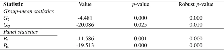
In Table 2 we present the WESTERLUND (2007) test results. We compute both asymptotic and robust bootstrapped p-values. The latter is making inference possible under very general forms of cross-sectional dependence.6 According to the group-mean and panel test statistics, we can strongly reject the null of no cointegration. This provides strong evidence of the presence of error correction for individual panel members and for the panel as a whole. We can say that

WESTERLUND’s (2007) cointegration tests shed light on the existence of a

long-run steady-state relationship between the variables entering the ERPT equation.

Table 2:WESTERLUND’s (2007) Panel Cointegration Test

Statistic Value p-value Robustp-value

Group-mean statistics

Gτ -4.481 0.000 0.000

Gα -20.086 0.025 0.010

Panel statistics

Pτ -11.586 0.001 0.000

Pα -19.513 0.000 0.000

Note:GτandGαare group mean statistics that test the null of no cointegration for the whole panel against the alternative of cointegration for some countries in the panel.PτandPαare the panel statistics that test the null of no cointegration against the alternative of cointegration for the panel as a whole. Optimal lag and lead lengths are determined by Akaike Information Criterion. In the last column, we present the bootstrappedp-values which are robust against cross-sectional dependencies. Number of bootstraps is set to 800..

4

Estimation of the long-run ERPT

Once the presence of cointegrating relationship is proved, we can obtain long-run ERPT coefficient by estimating equation 9 in levels. Following PEDRONI(2001),

we employ estimation techniques taking into account the heterogeneity of long-run coefficients. Therefore, FMOLS and DOLS Group Mean Estimator can be used to obtain panel data estimates for long-run pass-through. These estimators correct the standard pooled OLS for serial correlation and endogeneity of regressors

that are normally present in a long-run relationship.7 In our empirical analysis, we emphasize on between-dimension panel estimators. It’s worth noting that the between-dimension approach allows for greater flexibility in the presence of heterogeneity across the cointegrating vectors where the pass-through coefficient is allowed to vary.8 Additionally, the point estimates of the between-dimension estimator can be interpreted as the mean value of the cointegrating vectors, while this is not the case for the within-dimension estimates.9

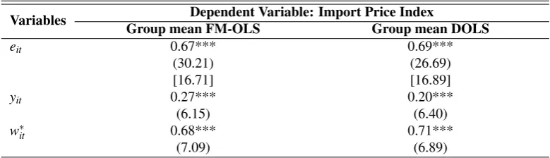
According to Table 3, long-run pass-through coefficient is statistically significant with the expected positive sign, and the results are fairly robust across estimation techniques. For instance, FM-OLS estimator suggests that one percent depreciation of the nominal exchange rate increases import prices by 0.67%. As we mentioned above, pass-through equation (9) assume unity elasticity of import prices to exchange rate movements in order to account for complete ERPT. However, the null of unity pass-through coefficient (H0:β =1) is strongly rejected through the different econometric specifications (seet-statistics reported between square brackets in Table 3).

Table 3:Panel Estimates for 27 OECD countries

Variables Dependent Variable: Import Price Index

Group mean FM-OLS Group mean DOLS

eit 0.67*** 0.69***

(30.21) (26.69)

[16.71] [16.89]

yit 0.27*** 0.20***

(6.15) (6.40)

w∗_it 0.68*** 0.71***

(7.09) (6.89)

Note: Group mean FM-OLS and DOLS estimators refer to between-dimension. These estimates include common time dummies. *** indicate statistical significance at the 1 percent level. Pass-through estimates are accompanied by twot-statistics. Thet-statistics in parentheses are based on the null of a zero ERPT coefficient (H0:β=0). Thet-statistics in square brackets are based on the null of unitary elasticity (H0:β=1).

This is an evidence of incomplete ERPT in our sample of 27 OECD countries. On the long run, import prices do not move one-to-one following exchange rate depreciation. These results are in line with estimates in the literature of exchange rate pass-through into import prices for industrialized countries. For 23 OECD countries, CAMPAand GOLDBERG(2005) find that the average of long run ERPT is 0.64%. In this study, producer-currency pricing (or full pass-through) assumption

7 _{Brief details of these methods are available in Appendix.}

8 _{Under the within-dimension approach pass-through elasticity would be constrained to be the} same value for each country under the alternative hypothesis.

9 _{According to PEDRONI(2001), the between-group FMOLS and DOLS estimators has a much}

is rejected for many countries. Using panel cointegration analysis, BARHOUMI

(2005, 2006) and HOLMES (2008) reject the pass-through unity for developing

countries. In accordance with the conventional wisdom that ERPT is always higher in developing than in developed countries, thus, a partial import prices is more expectable for OECD countries. As a matter of fact, one can think that pass-through would be complete in the long-run due to the gradual full adjustment of prices (as sticky prices tend to be a short run phenomenon).10 Nevertheless, some microeconomic factors like the pricing strategies of foreign firms can prevent a full adjustment of import prices following currency changes. Exporters of a given product can decide to absorb some of the exchange rate variations within their markups depending on market destination, i.e. by practicing a pricing-to-market strategy.11 This would explain why exchange rates are found to be much more volatile empirically than prices, and then pass-through would be incomplete even in the long-run. Also, our findings are in line with the theoretical price discrimination models which allow for a degree of pass-through lower than one even in the long run, as a result of pricing-to-market behaviour (See e.g. CORSETTI, DEDOLA, and LEDUC, 2005).

The evidence of partial ERPT in the long-run would have important policy implications. When imports prices do not fully respond to variation in exchange rate, this would reduce the sensitivity of trade flows to relative price changes, and consequently does not help external adjustment of the economy. For example, a depreciation of the importing country’s currency would reduce imports or promote exports less than expected, preventing a prompt adjustment of the trade balance. This outcome represent a key element in understanding the ongoing build-up of the global external imbalances. Moreover, our findings have also important implications for the design of monetary policy and the expectation of inflation. Import prices are a principal channel through which movements in the exchange rate affect domestic prices and hence also the variability of inflation and output. As is well-known, the successful implementation of monetary policy presupposes that central bankers have not only a good understanding of inflation dynamics, but that they are also relatively successful at predicting the future path of inflation. Then, the monetary authorities’ forecasts of the future path of inflation must be able to gauge how large are the effects of currency movements. If inflation forecasts are based on estimates that do not take into account for the incomplete degree of ERPT, these forecasts could be overestimating the effects of exchange rate variation on inflation.

10_{See e.g. SMETSand WOUTERS(2002).}

5

Conclusion

This paper has examined the long-run exchange rate pass-through (ERPT) into import prices for a panel of 27 OECD countries using panel cointegration approach. Previous empirical panel data studies have neglected the possibility of cross-sectional correlation and spillovers amongst countries. Since the strong economic and financial linkages between OECD countries cannot be ignored, we apply second generation panel unit root and panel cointegration tests which account for possible cross-sectional dependencies among the units included in the panel. We used PESARAN’s (2007) panel unit root test to determine the stationarity of panel variables. We find that all variables in levels to be integrated of order 1. Then, we tested whether variables entering the pass-through equation, i.e. import prices, the nominal exchange rate, exporters’ costs and demand conditions, are cointegrated. Using WESTERLUND’s (2007) tests for panel cointegration, our results suggest

the existence of a cointegrated levels relationship, as implied by the theoretical underpinning. When estimating the long-run pass-through coefficient, both FM-OLS and DFM-OLS estimators show an incomplete pass-through, i.e. import prices sensitivity to exchange rate movements does not exceed 0.70% for our sample of OECD countries. Especially, this outcome would explain the slow adjustment of trade flows to currency changes, even in the long-run, and help us in understanding the ongoing global external imbalances.

References

BAILLIU, J. and E. FUJII(2004), “Exchange rate pass-through and the inflation

environment in industrialized countries: An empirical investigation”, Working Paper No. 2004-21, Bank of Canada.

BANERJEE, A., M. MARCELLINO, and C. OSBAT (2004), “Some cautions

on the use of panel methods for integrated series of macroeconomic data”,

Econometrics Journal, Vol. 7, 322–340.

BARHOUMI, K. (2005), “Exchange rate pass-through into import prices in

developing countries: An empirical investigation”, Economics Bulletin, Vol. 3 (26), 1–14.

BARHOUMI, K. (2006), “Differences in long run exchange rate pass-through into

BREITUNG, J. and M. H. PESARAN (2005), “Unit roots and cointegration in panels”, inThe Econometrics of Panel Data, Matyas L. and Sevestre P., eds., springer-verlag berlin heidelberg edn.

CAMPA, J. and L. GOLDBERG(2005), “Exchange rate pass-through into import prices”,The Review of Economics and Statistics, 87 (4), 679–690.

CORSETTI, G., L. DEDOLA, and S LEDUC (2005), “Dsge models of high

exchange-rate volatility and low pass-through”, CEPR Discussion Paper No. 5377.

DE BANDT, O., A. BANERJEE, and T. KOZLUK (2008), “Measuring long run exchange rate pass-through”,Economics: The Open-Access, Open-Assessment E-Journal, 2 (2008-6).

GOLDBERG, P.K. and M. KNETTER(1997), “Goods prices and exchange rates:

What have we learned?”,Journal of Economic Literature, 35, 1243–72.

HOLMES, M. (2006), “Is a low-inflation environment associated with reduced

exchange rate pass through?”,Finnish Economic Papers, 19 (2), 58–68.

HOLMES, M. (2008), “Long-run pass-through from the exchange rate to import

prices in african countries”,Journal of Economic Development, 33 (1), 97–111.

IHRIG, J. E., M. MARAZZI, and A. ROTHENBERG(2006), “Exchange rate pass-through in the g7 economies”,Board of Governors of the Federal Reserve System, International Finance Discussion Paper, No. 851.

IM, K.S., H. PESARAN, Y. SHIN, and R.J. SMITH(2003), “Testing for unit roots in heterogenous panels”,Journal of Econometrics, 115, 53–74.

MENON, J. (1995), “Exchange rate pass-through”,Journal of Economic Surveys, 9, 197–231.

NEWEY, W. K. and K. D. WEST(1994), “Automatic lag selection in covariance

matrix estimation”,Review of Economic Studies, Vol. 61, 631–653.

PEDRONI, P. (1999), “Critical values for cointegration tests in heterogenous panels

with multiple regressors”, Oxford Bulletin of Economics and Statistics, 61, 653–678.

PEDRONI, P. (2001), “Purchasing power parity tests in cointegrated panels”,

PEDRONI, P. (2004), “Panel cointegration: Asymptotic and finite sample properties of pooled time series tests with an application to the ppp hypothesis”,

Econometric Theory, 20, 597–625.

PESARAN, M.H. (2007), “A simple panel unit root test in the presence of cross

section dependence”,Journal of Applied Econometrics, Vol. 22, 265–312.

SMETS, F. and R. WOUTERS (2002), “Openness, imperfect exchange rate pass-through and monetary policy”,Journal of Monetary Economics, Vol. 49, 947– 981.

WESTERLUND, J. (2007), “Testing for error correction in panel data”, Oxford

Bulletin of Economics and Statistics, Vol. 69 (6), 709–748.

Appendix. Estimation methods

A. FM-OLS Mean Group Panel Estimator

We consider the following fixed effect panel cointegrated system:

yit =αi+x

′

itβ+εit, t=1, ...T, (17)

x′_it, can in general be a m dimensional vector of regressors which are integrated of order one, that is:

xit = +xit−1+uit, ,∀i (18)

where the vector error process ξit = (εit,uit)

′

is stationary with asymptotic covariance matrix:

Ω_it = lim

T→∞E

h

T−1

∑

1ξit

∑

Ω0_i, is the contemporaneous covariance and, Γ_i, is a weighted sum of autocovariances.

The long run covariance matrix is constructed as follow:

Ω_11i Ω′_21i Ω_21i Ω_22i

, where,

Ω_11i, is the scalar long run variance of the residual,εit, and,Ω22i, is the long run

covariance among the,uit, and,Ω21i, is vector that gives the long run covariance

For simplicity, we will refer to,xit, as univariate. So according to PEDRONI

(2001), the expression for the group-mean panel FM-OLS estimator (for the between dimension) is given as:

ˆ

βGFM =N−1 N

∑

∑

(xit−x¯i)2

!−1

×

T

∑

t=1

(xit−x¯i)y∗it−Tγˆi

!

(20)

wherey∗_it = (yit−y¯i)−

ˆ

Ω_21i

ˆ

Ω_22i∆xit, and ˆγi≡

ˆ

Γ_21i−Ω0_21i−

ˆ

Ω_21i

ˆ

Ω_22i

ˆ

Γ_22i−Ω0_22i, with

yi=

1

T

T

∑

t=1

yit andxi=

1

T

T

∑

t=1

xit refer to the individual specific means.

The Pedroni between FM-OLS estimator, ˆβGFM, is the average of the FMOLS

estimator computed for each individual, ˆβFM,i, that is:

ˆ

βGFM =N−1 N

∑

i=1 ˆ

βFM,i (21)

The associatedt-statistic for the between-dimension estimator can be constructed

as the average of thet-statistic computed for each individuals of the panel:

t_βˆ_GFM =N−1/2

N

∑

i=1

t_βˆ_FM,i (22)

wheret_βˆ_FM

,i =

ˆ

βFM,i−β0

ˆ

Ω−₁₁1_i ∑T

t=1

(xit−x¯i)2

1/2 .

B. DOLS Mean Group Panel Estimator

The DOLS regression can be employed by augmenting the cointegrating regression with lead and lagged differences of the regressors to control for endogenous feedback effects. Thus, we can obtain from the following regression:

yit =αi+βixit+ Ki

∑

k=−Ki

The group-mean panel DOLS estimator is construct as:

ˆ

βGD=N−1 N

∑

∑

ZitZ

′

it

!−1

T

∑

t=1

Zity˜i

!

(24)

whereZit = (xit−x¯i,∆xit−K, ...,∆xit−K)is a the 2(K+1)×1 vector of regressors

and ˜yit=yit−y¯i.

The DOLS estimator for theith member of the panel is written as:

ˆ βD,i=

T

∑

t=1

ZitZ

′

it

!−1

T

∑

t=1

Zity˜i

!

(25)

So that the between-dimension estimator can be constructed as

ˆ

βGD=N−1 N

∑

i=1 ˆ

βD,i (26)

If the long-run variance of the residuals from the DOLS regression (23) is:

σ_i2= lim

T→∞E

T−1

∑

2

(27)

According to Pedroni, the associated t-statistic for the between-dimension

estimator can be constructed as:

t_βˆ

GD =N

−1/2

_∑

i=1

t_βˆ

D,i (28)

wheret_βˆ_D,i =

ˆ

βD,i−β0

ˆ σ_i−2 ∑T

t=1

(xit−x¯i)2