Munich Personal RePEc Archive
Convergence Clubs determined by
Economic History in Latin America
Barrientos Quiroga, Paola Andrea
School of Business and Social Sciences, Aarhus University
August 2013
Online at
https://mpra.ub.uni-muenchen.de/50191/
1
Convergence Clubs determined by
Economic History in Latin America
Paola A. Barrientos Quiroga
Abstract
2
1
Introduction
The detection of income disparities across clubs of economies can help determine how to speed up
the process of economic development and understand the sources of differences in growth
performances. In theory, the reasons behind club convergence could be several, among these: the
existence of some threshold level in the endowment of strategic factors of production,
non-convexities or increasing returns, similarities in preferences and technologies, and government
policies and institutions (Canova, 2004; and Azariadis, 1996). Empirically, there is no unified
agreement on how to identify clubs. Most researchers (e.g. Durlauf and Johnson, 1995; Paap and
Van Dijk, 1998; Desdoigts, 1998; Hansen, 2000; Canova, 2004; Owen, et al., 2009) lean towards
the approach of letting the data decide the clubs. They usually study the shape of the distribution of
income (or capital) and focus on finding an income (or capital) threshold to divide countries into
clubs, or the thresholds are determined beforehand. However, the division of clubs by income (or
capital) is not very informative with respect to the forces behind the heterogeneity in income (or
capital) in first place.
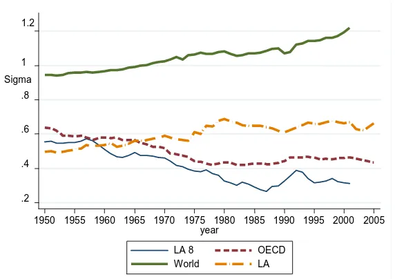
Although Latin America is typically considered a club itself, due to its common characteristics,
such as language, geography, religion, history and policies, it exhibits differences across countries
(see Figure 1). Dispersion in GDP per capita has been increasing on average over the period
1950-2005 in Latin America, whereas it has been decreasing among the OECD countries. Then a relevant
question is, Why diversity in growth trajectories in a region with so many common roots? Some
candidates for an explanation come to mind: commodity lottery/geography, poor market integration,
colonial heritage, and differences in economic policies, among others.
Some researchers have gone far in time to explain the diversity in development paths in Latin
America and the connection to institutions. Acemoglu, Johnson and Robinson (2001) find that there
is a strong correlation between early institutions and institutions today. In the specific case of the
Americas they distinguish between regions that were settled by Europeans and regions that, due to
high settler mortality, the Europeans established “extractive states” instead. The latter model paved
the way for extractive states even after political independence in the nineteenth century. In a later
3
and economic institutions of the conquistadors have endured and condemned much of the region to
poverty. There are, however exceptions. Argentina and Chile have fared better than most. Because
they had few indigenous people or mineral riches (exploitable at the time) they were “neglected” by
the Spanish. Consequently, there are differences even in this dismal picture of colonial heritage.
Similarly, Engermann and Sokoloff (2002) argue that institutions are endogenous, and that the roots
of the disparities in the extent of the inequality that we observe today lay in the initial factor
endowments. Through comparative studies of suffrage, public land and schooling policies they
document systematic patterns by which the societies in the Americas, that began with more extreme
inequality or heterogeneity in the population were more likely to develop institutional structures that
greatly advantaged members of the elite by providing them with more political influence and access
[image:4.595.164.450.387.589.2]to economic opportunities.
Figure 1. GDP per capita dispersion in the World, OECD, Latin America and eight Latin American countries (LA8 - Argentina, Brazil, Chile, Colombia, Mexico Peru, Uruguay and Venezuela). Standard deviation of the logarithm of GDP per capita.
Empirical research on convergence in Latin America is still scarce compared to other regions1, and only one other study incorporates economic history features into the analysis: Astorga et al.
(2005). They do a time-series analysis for each of their six countries of study, during 1900-2000,
1 There are only nine cross-country studies on convergence: Blyde, 2005 and 2006; Holmes, 2005; Astorga et. al., 2005;
Dobson and Ramlogan, 2002a and 2002b; Utrera, 1999; Dabus and Zinni, 2005; and Madariaga et.al, 2003.
.2 .4 .6 .8 1 1.2
Sigma
1950 1955 1960 1965 1970 1975 1980 1985 1990 1995 2000 2005 year
LA 8 OECD
4
where they find different breaks for each of them. They conclude that there are two external shocks
affecting the six economies simultaneously: in the 1930s due to the Great Depression and in the
1980s due to the shift in US monetary policy and debt crises2. They find convergence between the six countries by using panel data and error correction models, and conclude, among other things,
that there is convergence among the six countries but it seems there is divergence between the rest,
forming two distinct convergence clubs (they do not test for this). They say that the "rest" show an
inferiorpattern of growth compared to the six, due to lower growth rate and greater vulnerability,
which may possibly relate their greater vulnerability to the external shocks.
This study pretends as well, to answer the question posted earlier of why diversity in growth
trajectories in a region with common roots and fill in the gap in the literature by analyzing,
empirically, the existence of club convergence in 32 Latin American countries over more than 100
years, more than any other study.
I analyze club formation in a different way than the conventional procedures (income or capital
threshold determination) and incorporate the institution link to growth. I examine sources of
heterogeneity on the basis of economic history, which informs us on the different initial
endowments, the most important common external shocks and the policy-responses. Such historical
events shape the way institutions are formed, and institutions determine the way scarce resources
are used. As mentioned by Easterly (2003), technology is endogenous to the institutions that make
adoption of better production techniques likely. The institution link in terms of Acemoglu and
Robinson (2012) and Engerman and Sokoloff (2002) enters in the analysis when I, first, divide the
clubs according to their factor endowments. However, after the external shocks hit the region, a mix
of countries of different endowments try to change their pattern of development while others remain
in the same path. In other words, I recognize that there is a legacy from the colonizers but I also
accept that external shocks and certain circumstances can also change this legacy by the decision
and possibilities of the policy makers.
The criteria of division of clubs follow three steps. First, I identify the main common external
shocks that changed the development patterns in the region: the Great Depression in 1930s and the
2 However, from my point of view, the shift in US monetary policy and debt crises are consequences of the exogenous
5
oil price shock in 1974. Then, I classify countries in clubs according to first, their initial endowment
of natural resources and then according to their policy-response to the shocks. Here, I focus on
information of the policies rather than outcomes so that the results are not driven by the selection of
the club thresholds in the first place. Finally, I test for convergence within each club.
Before 1930, I define two clubs according to their exporting product: the mineral and
agricultural producers. After the Great Depression I follow Diaz (1984) classification of clubs,
according to passive or reactive countries, where the reactive responded autonomously to protect
themselves, while the passive did/could not. After the oil price shock, I classify the clubs according
to the Lora index (Lora, 2001), which describes to what extent countries applied structural reforms
to liberalize their economies. I also have the Caribbean countries as a separate club.
In connection to growth theory, under multiple-equilibria models, each historical watershed
represents an opportunity to modify the set of initial conditions and to escape from a development
trap, whereas in the Solow model approach, those historical points represent critical changes in
policy parameters and a redefinition of the steady state. The empirical analysis cannot distinguish
between these two kinds of models.
The following section discusses the background of the paper. First it discusses the theoretical
aspects behind club convergence, then it summarizes the prior research in Latin America, and
finally it reviews the common economic history events in the region. Section 3 describes the
empirical specification of the paper, which consists of the division of clubs and the econometric
specification. Section 4 presents the results and Section 5 discusses the strengths and weaknesses of
the approach. Finally, I present the conclusions. The data details are presented in the appendix.
2
Background
2.1
Connection to theory: from the Solow-Swan model to multiple
equilibrium models
The concept of economic convergence has been discussed through many years since Ramsey
6
growth theories3, but instead it discusses and compares, in general terms and briefly, the two most important theories behind club convergence that emerge from the most basic version of
Solow-Swan model and the multiple equilibria models.
The neoclassical growth models, of which the simplest version is Ramsey-Solow model, arrive
at a growth equation where convergence can be estimated by4,
. log ( / ) = − ∙ log ( ∗/ ) + (1)
where the average growth rate in the interval from 0 to T for country i, . log ( / ), is related negatively to the initial output in relation to the steady state output ∗, and positively to
the technology growth x, while keeping β (speed of convergence) and T (period) constant.
Equation (1) describes conditional β-convergence in the sense that a poor country A will grow faster than rich country B, understanding that country A is poorer because it is further away from its
own steady-state than country B is. In contrast, absolute β-convergence assumes that ∗is the same for country A and B, ∗= ∗. We cannot know exactly what the steady state output looks like, but
we know it is related to structural characteristics such as technologies, preferences, propensity to
save, institutions, policies, etc.
Empirically, one can estimate β-conditional convergence by finding proxies for the steady state5 or by grouping economies that we assume have the same steady state (Sala-i-Martin, 1996). So, if
we gather countries that have or we expect to have similar steady-states we are finding (or testing
for) convergence in different groups, namely group convergence.
On the other hand, the multiple equilibria models starting with Azariadis and Drazen (1990)
(and followed by many others, see Durlauf and Quah, 1999) advocate for multiple regime in which
different economies obey different linear models when grouped according to different initial
conditions. For example, there exists a range of human or physical capital levels over which the
3
Durlauf and Quah (1999) offer a great summary of economic growth theories and empirics
4
Basically, from a Cobb-Douglas production function for the economy, and a Utility function for a representative agent, the economy will eventually arrive to a steady state, where the economy cannot grow anymore. Equation (1) is the resulting equation after optimization and log-linearlization (see Barro and Sala-i-Martin (2004) for the derivations).
5 However, the problem of adding controls as proxies for the steady-state, is that these will probably be endogenous
7
aggregated production function is not concave which will lead to different long-run steady-states. In
this way, initial conditions can “trap” countries into not reaching the rich countries.
Azariadis (1996) and Canova (2004) suggest that the potential causes of traps are several, like
technologies, preferences, market structures, fertility patterns and public policies. These variables
preserve and augment initial inequality in per capita income among otherwise identical national
economies. This concept is called club convergence.
Unfortunately, economic theory does not guide us on the number of clubs or the way in which
the different variables defining initial conditions interact in determining the clubs. To address this
issue, most researchers (e.g. Durlauf and Johnson, 1995; Bai, 1997; Hansen, 2000; Pesaran, 2006;
Paap van Dijk,1998; and Desdoigts, 1998) lean towards the approach of letting the data decide the
clubs. They usually study the shape of the distribution of income per capita and focus on finding an
income threshold to divide clubs; however they may not be able to explain the differences in income
or capital in first place.
The difference between group convergence and club convergence lies on their assumption about
stratification. Group convergence assumes the stratification is due to different steady states, while
club convergence assumes that the stratification comes from interactions on initial conditions with
different variables. Empirically, both can be estimated from Equation (1).
2.2
Prior research in Latin America
In Latin America, there are only nine cross-country empirical studies6 on convergence (Blyde, 2005 and 2006; Holmes, 2005; Astorga, et.al 2005; Dobson and Ramlogan, 2002a and 2002b;
Utrera, 1999; Dabus and Zinni, 2005; and Madariaga et.al,2003). Although they analyze the same
region, they study different countries and periods, and apply different methodologies.
Some of the authors use methodologies that do not measure a specific speed of convergence,
such as Blyde (2006), who studies 21 countries during 1960-2004 and uses a distribution dynamics
approach. He finds that countries are converging to two clubs; one large for low and low-middle
6
8
income countries and another small for rich-income countries. The high-income countries are
Uruguay, Argentina, Chile, and Mexico, and the remaining 17 countries are in the other club.
Dobson, Goddard and Ramoglan (2003) study the case of 24 countries during 1965-1998 by
using cross-section analysis and unit root with panel data tests, and find convergence but not a
specific speed nor different clubs. Other researchers find concrete results but no clubs. For
example, Dobson and Ramlogan (2002a and b) study 19 countries and 28 and 30 years, respectively
(1970-1998 and 1960-1990), using cross-section regression and panel data analysis, and find speeds
of convergence of 0.02% to 2%7. Helliwell (1992) analyzes 18 Latin American countries over the period 1960-1985 and finds convergence at a speed of 2.5%8.
The only other study that incorporates economic history features into their analysis is Astorga et
al., 2005. They first do a time series analysis for each of their six countries of study, during
1900-2000, where they find different breaks for each of them. They conclude that there are two external
shocks affecting the six economies simultaneously: in the 1930s due to the Great Depression and in
1980s due to the shift in US monetary policy and debt crises9. Later, they find convergence between the six using panel data and error correction models, at a speed between 1% and 1.9%, where the
oscillation comes from the addition or subtraction of explicative variables that proxy for the steady
state10. They conclude, among other things, that there is convergence among the six countries but it seems there is divergence between the rest, forming two distinct convergence clubs (they do not test
for this). They say that the "rest" show an inferior pattern of growth compared to the six, due to
lower growth rate and greater vulnerability, which may possibly relate their greater vulnerability to
the external shocks.
In stark contrast to these findings of relatively low speeds of convergence, Dabus and Zinni
(2005) analyze 23 countries from 1960 to 1998, and find absolute and very high conditional
convergence rates. The authors argue that once controls are introduced and extremely high speeds of
7
Their studies include, as proxies for the steady state, sectorial decomposition variables, country dummies, population growth, savings, and human capital.
8
He includes variables such as investments, population growth, human capital, and scale effects.
9
However, from my point of view, the shift in US monetary policy and debt crises are consequences the exogenous shock of the increase in oil prices in 1974.
10
9
conditional convergence are found, compared to absolute convergence, then it is a signal of
divergence. This is a good point, since when controlling for many characteristics, a hypothetical
speed of convergence is being calculated, while the real speed of convergence would be the one
closest to absolute convergence11. They conclude that convergence of any type is absent in Latin America.
2.3
Economic history of the region
To analyze the economic history of 32 countries during more than 100 years is a complicated
task, and even more so when one wants to focus on the common factors of the region as a whole
rather than country specific sets of events. Historians face this task, and one of the main references
for my analysis in this section is Thorp (1998), who captures in depth the comparative reality within
Latin America.
Below, I describe the common events and focus on two very important external shocks that have
changed the development patterns in the region: the Great Depression of 1930 and the oil crisis in
1974. The first shock changed the political economy of the region, and as a result many of the
countries underwent a process of import substitution industrialization. The second shock, too,
changed the political economy of the region, resulting in a debt crisis, to which the response in
many cases was to adopt structural reforms to liberalize the economies. Thus, the pattern changed
from initially exporting, to substituting imports with the state playing an important role, and finally
liberalizing and a lowering the role of the state.
1900-1930: The Exporting Phase
There is no doubt that during the first phase of the 20th century the economics of the region was
characterized by being dependent on exports, which were primary products with low value added.
The region was vulnerable to world income and to fluctuations in primary products prices.
The first phase is characterized by the world export demand being high and the capital flows
being fluent to the region. These two facts determined the way Latin America developed. The
11
10
region exported the needed primary products and at the same time imported more elaborated goods
produced in the "center".
WWI (1914-1918) accelerated the shift in trade and investment structures in the region. The
demand for Latin America’s exports increased, and according to Furtado (1981) the war stimulated
the industrial growth in the region, especially in the mineral countries. The economic pattern and the
political economy did not change after WWI, but they did when the Great Depression hit the region.
1930: The Great Depression
In 1929 the US stock market crashed and provoked a fall in economic activity in the
industrialized countries, which in turn reduced their demand for primary products and reversed the
capital flows to Latin America. This situation deteriorated the terms of trade of all primary products,
leading to an increase of the Latin American real import prices. The natural mechanism of
adjustment is a decrease in real export prices so that demand is stimulated again, but due to the
extreme circumstances of the Great Depression, world demand could not recover. Instead, Latin
American demand went from imported manufactured goods to domestic manufactured products.
This process stimulated the import substitution phase of Latin America. Cardoso and Helwege
(1992) call it "import substitution by default".
The process of industrialization via import substitution was reinforced by WWII (1939-1945).
Although WWII brought an increase of Latin American exports, there were constraints on imports.
Consequently, the scarcity of imports and the deterioration of terms of trade of primary products
encouraged new efforts to substitute imports, but these efforts were in turn limited by scarcity of
imported inputs and capital goods. National governments promoted industries and restricted
imports, mainly by lowering interest rates, giving easy credits, and controlling prices. Capital
inflows were attracted through loans to the public sector. Moreover, governments applied multiple
exchange rates, protective tariffs, import licenses, and different import quotas that could favor the
essential goods imports and reduce final goods imports.
As a result of the protection of the national markets, the exporting sectors in many countries in
Latin America were discouraged due to high cost of domestic intermediate products, and the
11
Moreover, fiscal revenues from the commodity product sector went down and public spending rose,
creating a fiscal gap, which in some cases was monetized and later created persistent inflation. The
result was detrimental for sectors that were not intensive in capital, like the agricultural sectors and
the artisans. Finally, the low interest rates given by the government to promote investments
discouraged saving even when helping inefficient firms and corruption increased greatly. However,
for those countries where industrialization was strong, innovations were made in terms of
organization, technology and R&D (together with investment in education), like in Brazil,
Argentina and Mexico. Another positive side was that some enterprises were ready to export.
Overall, more manufactured goods were produced.
1974: Oil Price Shock
Later, in 1974, the shock of the increase in oil prices led Latin America to become highly
indebted, which led to a debt crises in the region. The mechanism is described by Cardoso &
Helwege (1992) as follows: "..Oil exporters deposited their earnings in the commercial banks of
developed countries, but higher oil prices caused a recession in OECD countries and reduced the
demand for credit. Left with excessive liquidity bankers eagerly lent to the Third World at very low
interest rates.." .
The debt crises started in 1979 and 1981 when the Unites States and other OECD countries kept
their money supply tight and increased interest rates radically. Since countries acquired loans at
floating interest rates, their debt obligations increased very much12. The adjustment of the debt crises was costly for all countries in the region, mainly due to the massive capital outflow.
Governments were not able to continue their policies and had to make drastic changes. In general,
governments printed more money to cover or keep their fiscal deficits constant. With all the
borrowed money, governments were used to spending more than their incomes. Since printing
money can cause inflation pressures and damage real wages, some governments indexed the
nominal wages to prices to keep real wages constant. Speculators, trying to earn from the
indexation, raised prices at higher rates than salaries. Sooner or later inflation exploded into
hyperinflation and governments were no longer able to manage it.
12
12
Countries were desperate to stabilize and gain access to foreign credit again, and the
"Washington Consensus policy package" was an option to reach stabilization. The package was a
set of structural reforms to liberalize the economy. The specific policies were to cut budget deficits
(by reducing expenses and increasing taxes), privatize, liberalize imports, impose exchange controls
(devaluate), eliminate price controls (to reflect the real costs), and increase interest rates (Cardoso &
Helwege, 1992). Some countries took the package as such, and others took some elements of it.
However, in general the adjustment left behind common problems that reinforced each other, such
as capital outflows, fiscal deficits, inflation, overvaluation, and balance of payment crises.
Later, in the 90’s, some trends of thought support the idea that good institutions create
complementarities between productivity growth and equality. Others maintain that policies that are
linked to the political constituency will create a combination of economic and social development.
When the population participates in the process of making decisions, the feeling of ownership helps
to monitor and accomplish their obligations better. Thorp calls these new currents "the New
Paradigm Shift", which started by the mid 1990s, as a response to the poor welfare results. Thorp
points out that the rise of the paradigm shift is a result of the increasing capital flows, the debt
crises, and the costly adjustment process. However, it is hard to attribute the results to either
globalization or policy shifts alone.
3
Empirical Specification
The previous section described how the political economy changed from initially exporting, to
substituting imports with a great role played by the state, and finally to liberalizing and a
diminishing the role of the state. These changes are clearly radical, and according to multiple
equilibria models, each historical watershed is an opportunity to modify the set of initial conditions
and to escape from a development trap and according to Solow-Swan model, each political change
will result in different steady-states.
I focus on a criterion to divide countries into clubs that describe the initial conditions after the
shocks, as under the multiple-equilibria models. The criterion is based on the policies adopted at the
13
outcomes so the results are not driven by the selection of the club thresholds in the first place13. I explain first the club division and later the econometric specification.
3.1
Division of Clubs
Mineral and Agricultural Clubs: 1900-1930
For the first phase, the initial conditions are defined in terms of type of natural resource
endowment. Due to lack of data in this phase, I divide countries into groups according to mineral vs.
agricultural countries, rather than a more extensive type of division by product.
Agricultural countries’ production was vulnerable to natural disasters, and minerals were
vulnerable to recessions in the "center", because minerals were used in construction, machinery, and
chemicals production. Moreover, the two types of production had different spillovers. For instance,
the mining sector was characterized by using less land and labor with more capital and
technological intensity, and having different transport needs than the agricultural sector. Acemoglu
et.al (2001) also points out that the mining countries set more extractive institutions.
The agricultural countries are: Brazil, Colombia, El Salvador, Nicaragua, Costa Rica,
Guatemala, Honduras, Ecuador, Cuba, Argentina, and Uruguay. They were mainly producing
coffee, bananas, cacao, sugar, meat, and/or wheat. Those mainly producing coffee were Brazil,
Colombia14, El Salvador and Nicaragua. Costa Rica and Guatemala were mainly producing coffee and bananas, while Honduras was producing bananas and precious metals. Cuba mainly produced
sugar, but also tobacco. Argentina and Uruguay were mainly producing meat and wheat.
The mineral countries numbered four: Chile, Mexico, Peru, and Venezuela. They exported
mainly petroleum and copper. Petroleum was produced by all except Chile, and copper was
produced by all except Venezuela. Before 1917, Venezuela was mainly producing coffee and cacao,
but after that year petroleum became the most important source of revenue15. Mexico was the most
13
In Barrientos (2010), I actually analyzed different clubs in the region based on the outcomes rather than the policies.
14
Colombia also exported gold (Antioquia region) besides coffee but I keep it in the agricultural group because coffee has been more traditional.
15
14
diversified export country in Latin America, also exporting lead, zinc, silver, gold, coffee, rubber,
and cotton. It discovered its oil in 1910.
Reactive and Passive Clubs : 1931-1974
After the onset of the Great Depression in 1930, countries responded in different ways. Díaz
(1984) divides countries into reactive and passive. The reactive countries had policy autonomy in
the sense that they could, for example, depreciate their exchange rate and thereby speed up the
relative price adjustment to recover faster, while the passive countries had to stay tied to the dollar.
Also monetary and fiscal policies were employed. Some countries were not included in Díaz (1984),
so I use Taylor (1999) to complete the clubs. Those countries that did some sort of exchange rate
control and market activity control were included in the reactive club16.
Díaz (1984) classified as reactive countries: Argentina, Brazil, Chile, Colombia, Mexico, Peru,
and Uruguay. I added to this group six countries that were not mentioned by Diaz (1984) but by
Taylor (1999): Bolivia, Costa Rica, Nicaragua, Paraguay, and Venezuela. According to Table 3 in
Taylor (1999), these countries exerted some sort of exchange rate control and/or some sort of
control of capital market activity.
Diaz (1984) has the following passive countries: Cuba, Dominican Republic, Honduras, Haiti,
Panama, and Puerto Rico. I added Ecuador, Guatemala, and El Salvador, following Taylor (1999).
Low and High Reformers Clubs: 1975-2007
After the oil prices shock in 1974, countries went into debt crises, and the policy decision was
whether to follow the structural reforms proposed by the Washington consensus or not. The change
in policies was very radical in the region. Many countries went from protection of national markets
and great control by the state to policies that facilitate the operation of markets and reduction of the
distorting effects of state intervention in economic activities. Lora (2012) develops an index that
tries to capture how deep the reforms went (rather than outcomes). The higher the index, the more
market friendly the reforms. The index summarizes the status of progress in policies within trade,
financial, tax, privatization, and labor areas. By using the Lora index, I classify countries into two
16
15
groups: the high reformers, whose indices are above the average, and the low reformers, whose
indices are below average17.
According to the Lora index the high-reformers are: Argentina, Bolivia, Chile, Panama,
Paraguay, and Uruguay. I added to this group Panama and Puerto Rico, given that both have close
relations with USA who promoted the Washington Consensus package.
According to Lora's index, the low-reformers are: Brazil, Colombia, Costa Rica, Dominican
Republic, Ecuador, Guatemala, Honduras, Mexico, Nicaragua, Peru, and El Salvador. I added Cuba
for obvious reasons.
Caribbean Club
Finally, the Caribbean countries are treated as one club, due to its own characteristics. They are
small, dependent on USA, and are characterized by their vulnerability to capital flight and
international interest rate changes. They are quite open18 and primary products producers. Additionally, Caribbean countries are exposed to natural disasters. I include the Caribbean club in
each phase except the first due to lack of data.
The Caribbean group consists of many islands and English speaking countries, mainly part of
the trade union CARICOM: The Bahamas, Barbados, Belize, Dominica, Grenada, Guyana, Haiti,
Jamaica, Saint Lucia, St. Kitts and Nevis, St. Vincent and the Grenadines, and Trinidad and Tobago.
3.2
Econometric Specification
The model setup follows Barro and Sala-i-Martin (2004), where the main interest is in
measuring the non-linear relation between initial output and growth. Although the setup is
developed for neoclassical growth models, it is used when measuring club convergence as well.
I start from the absolute convergence definition:
= − #" !"∙ $"+ (2)
17
The Lora index of structural reforms is taken from the year 1985, while phase 3 starts in 1974. I considered starting the last phase in 1985, but then I would be inconsistent with the previous phase, where the break was determined by an external shock. One could argue that the increase in US interest rates in 1979 was the external shock, but this in turn was a response to the oil price shock earlier. Also from 1974 to 1979 the results should not change significantly.
18 In the 1990s, 19 of the 26 Caribbean states had a ratio of Exports and Imports to GDP of more than 100 percent (Thorp,
16
where subscript i refers to countries, i=1,...N and t refers to periods, t=1,...T. Each period has a
length of %, which is determined by the availability of data19, is the growth rate of GDP per capita over the period, $" is the initial output per capita (measured in logarithms), is a
constant20, β is the speed of convergence if β>0 (or divergence if β<0), and is the disturbance term.
Equation (2) tells us that if β is positive, the relation between initial income and growth is
negative, so that the poorer the country is at the beginning, the faster the growth rate, which implies
that the differences at the beginning of the phase tend to disappear.
Galor (1996) mentions that by adding empirically significant elements to the neoclassical growth
model, one can analyze club convergence under the same framework, he suggests inequality
measures as an example. So, in order to control more adequately for the initial differences, I add
two more variables at the beginning of each period: size and ranking of each country. Size could
give a certain advantage in the growth process, since size is associated with economic power. In a
similar fashion, position in the distribution of income captures the relative ranking at the beginning
of the period:
= −1 − '% (!"∙ $"+ ) *+∙ +$"+
,
(3)
where $" is the size of a country measured by the logarithm of population and , $" is the
ranking measured by the relation of each country’s output per capita to the highest output of the
same year.
Now, I introduce the two main external shocks discussed earlier:
= − #" !"∙ $"+ ∑+-, *+∙ + $"+∑,0- /0∙ 10$"+ (4)
19
Details on τ are in the appendix.
20
17
where 1 is a dummy for the first phase 1900-1930, 1, for 1931-1974, and 12 for1975-2007.
The next step is to introduce a dummy for each club. I create dummies where I combine phase
and club characteristics. I replace the phase dummies with club dummies:
= − #" !"∙ $"+ ∑+-, *+∙ + $"+∑64- 34∙ 54$"+ (5)
where 54$" is the club dummy. In total we have eight dummies (c=1,...8) that represent the clubs
mentioned in the previous section. In Phase 1 we have the agricultural and mineral clubs, in phase 2
reactive and passive clubs, and in phase 3, high-market friendly and low-market friendly countries.
Moreover, we have the Caribbean countries as a club and included for phases 2 and 3.
Equations (2) to (5) describe general aspects for the region as a whole. Only one common β
coefficient is included. So, after controlling for the different dummy characteristics, we get one beta
for the entire region. Additionally, we can see the significance of each club in the overall growth
and compare their contribution.
Next, I focus on finding different β coefficients, one for each club. I first calculate a similar
version of Equations (2) and (3) with a different β for each group:
= − 7 ∑=9>?A<89 ∙:9;<∙@< ⋅ y ;<+ uEF (6)
= − 7 ∑=9>?A<89 ∙:9;<∙@< ⋅ y ;<+ ∑,+- *+∙ + $"+uEF (7)
and then adding the phase dummies to Equations (6) and (7):
18
= − 7 ∑=9>?A<89 ∙:9;<∙@< ⋅ y ;<+ ∑,+- *+∙ + $"+∑20- /0∙ 10$"+uEF (9)
Since it is a costly model in terms of parameter estimation, I restrict the parameters *+ to be
equal across clubs. I also restrict the model to have only three (phase specific) constants instead of
eight different (club) constants. Moreover, the interest lies in the initial income coefficients, and
here the club effect is allowed. I prefer not to do a separate regression for each club since the panel
data sample for each club becomes too small.
4
Results
The econometric tool employed is non-linear pooled OLS regressions for 32 countries for the
period 1900 to 2007. The data description is in the Appendix. I report the coefficients,
heteroskedasticity consistent standard errors (White, 1980) and other descriptive estimates, from
Equations 2-5 in Table 1 and from Equations 6-9 in Table 2.
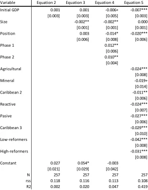
From Table 1 we can see that the initial income coefficient, β, has almost the same rate in
Equation 2 as in Equation 3: around 0.15%. However, in both cases we fail to reject the null
hypothesis that the β coefficient is zero (no convergence). When adding size and position, Equation
2, the coefficient of the variable size is significant and negative, while the coefficient for the
variable position is positive but insignificant.
Equation 4 shows that each of the phase dummies is significantly different from the last phase
(the omitted dummy). I also test whether both phase dummies are jointly significant in the equation
(H₀: c₁=c₂=0). The test statistic is F=3.25, and we reject the null (at a level of 95% of confidence).
The β coefficient is -0.65%, showing overall divergence. The coefficient of size remains negative,
while position has changed to negative. Both variables are significant.
Equation 5 substitutes the phase dummies for the club dummies, since the last ones include the
first ones. Results are in the last column of Table 1. Regarding β, there is a significant negative
coefficient, supporting divergence among all Latin American countries. This means that the relation
19
clubs and initial conditions. All coefficients of club dummies are significant, except for the mineral
countries. This is clear evidence that the club division is successful. The coefficients of all dummies
are negative, which is just showing the differences in the constant term of the growth equation
according to the clubs. Size and position retain negative signs.
So far, I have shown that the division of phases and clubs is very important, and that there is
significant divergence among all countries, after controlling for differences in initial conditions and
membership in different clubs.
The next task is to see whether contrary to the overall divergence picture there is in fact
convergence inside each club. We proceed to calculate β convergence for each group. Table 2
shows the results from estimations of Equations 6 to 9.
Equation 6 is a similar version to Equation 2, in the sense that no controls are included. The
results are presented Table 2. The βs for all clubs are significant and positive. This supports again
the basic idea behind the paper, that there is club convergence, and the coefficients are significant.
The positive sign of β means that there is a non-linear negative relation between initial income and
growth. All coefficients are low and similar to each other, so I test whether the club dummy
coefficients are significantly different from each other, and whether they are jointly significant. The
F test is 3.54 for the first test indicates that we can reject the null with 95% confidence, and
similarly, F=3.48 for the second test, which means that the dummies are jointly significant and
different from each other. To control for more initial conditions, Equation 7 is estimated. The results
in column 2 show that the βs remain similar, all positive and significant. I do the same tests as for
Equation 5, and the results show that all βs are jointly significant and significantly different from
each other. The coefficient for size is still negative and for position positive, but both insignificant.
In general, the results show that the division by historical phases and clubs is important. When
the club dummies were introduced in the specification, where it was assumed that β was common in
the clubs, in Column 4 Table 1, the club dummies were significant, so that their inclusion was
correct, and the β coefficient that relates initial income to growth was negative, which means
divergence among all countries (confirming the impression in Figure 1). After allowing for
heterogeneity in the non-linear relation between growth and initial income, in Table 2, there is
20
as expected (Columns 1 and 2 in Table 2). When adding more controls, two of them become
insignificant, the Caribbean and the high-reformers (Columns 3 and 4 in Table 2) in the last phase.
The two variables besides income, used to control for differences in the initial conditions, size in
terms of population, and position in the income distribution, show a negative relation with growth
when significant (Columns 2 to 4 in Table 1). The rates of speeds of convergence are all around
0.5% which is lower than the typical 2% found in the literature. The reason for this difference may
21
Table 1. Common β. Econometric results from estimations of Equations 2 to 5. Standard errors in brackets, *** significant with p<0.01, ** p<0.05, *p<0.10, ++p<0.15 and +p<0.20. Phase 3 is omitted
Variable Equation 2 Equation 3 Equation 4 Equation 5 Initial GDP 0.001 0.001 -0.006+ -0.007***
[0.003] [0.003] [0.005] [0.003]
Size -0.002** -0.002** 0.000
[0.001] [0.001] [0.001] Position 0.003 -0.014* -0.020*** [0.006] [0.008] [0.006]
Phase 1 0.012**
[0.006]
Phase 2 0.010**
[0.004]
Agricultural -0.024***
[0.008]
Mineral -0.019+
[0.014]
Caribbean 2 -0.011**
[0.006]
Reactive -0.024***
[0.007]
Pasive -0.027***
[0.006]
Caribbean 3 -0.029***
[0.010]
Low-reformers -0.042***
[0.008]
High-reformers -0.031***
[0.008] Constant 0.027 0.054* -0.003
[0.021] [0.029] [0.042]
N 257 257 257 257
22
Table 2. Different β rates. Econometric results of estimations of Equations 6 to 9. Same description as Table 1. Variable Equation 6 Equation 7 Equation 8 Equation 9
Initial GDP
Mineral 0.004* 0.004* 0.000 -0.001 [0.002] [0.002] [0.006] [0.007] Agricultural 0.004*** 0.004*** 0.001 0.000 [0.001] [0.001] [0.006] [0.008] Caribbean 2 0.002* 0.002* 0.002** 0.002** [0.001] [0.001] [0.001] [0.001] Reactive 0.004*** 0.004*** 0.005*** 0.004*** [0.001] [0.001] [0.001] [0.001] Pasive 0.004*** 0.004*** 0.005*** 0.005*** [0.001] [0.001] [0.001] [0.001] Caribbean 3 0.003*** 0.004** 0.001 0.000 [0.001] 0.002 0.004 0.005 Low-reformers 0.005*** 0.005*** 0.003 0.001 [0.001] [0.001] 0.004 0.006 High-reformers 0.003*** 0.004*** 0.001 0.000 [0.001] [0.001] 0.004 0.005
Size -0.001 -0.001
0.002 0.002
Position 0.003 -0.002
0.006 0.007
First Phase 0.021 0.029
0.041 0.064
Second Phase 0.055*** 0.064** 0.010 0.029
Third Phase 0.027 0.028
0.036 0.045 Constant 0.046*** 0.056**
0.009 0.028
N 257 257 257 257
rss 0.109 0.109 0.109 0.109
23
5
Strengths and Weaknesses of Approach
Even though the results are quite satisfactory, there are caveats regarding the approach that need to
be discussed. In this section I discuss the flaws of the current division of clubs, other possible ways
of finding clubs, omitted variables, unbalanced panel data, and measurement errors.
5.1
Division of Clubs
The most controversial characteristic of this paper is the division of clubs. There could have been
superior alternative ways to approach the division.
Ideally, I could have determined structural breaks for the given time period of data for all 32
countries. One way of doing this is following Bai (1997), who develops a method for finding
multiple breaks. Another option is to analyze breaks for each country and see if there were common
breaks. Astorga et al. (2005) do this for six countries over 100 years, using the Chow test. Table 1 in
their paper shows the different structural breaks by country. These shocks account for external and
internal events, like revolutions, dictatorships, and country specific characteristics. At the end, the
authors do a panel data analysis where they recognize that the major events for all countries were
the crisis of 1929 and its aftermath in 1930, along with the debt crises in the 1980s. Instead, I let
historians decide the breaks, and, after all, the breaks are similar to the ones in Astorga et al. (2005).
Moreover, the significance statistical tests on the phase dummies prove that the breaks are relevant.
Similarly, regarding the clubs, I could have chosen many other ways of dividing countries into
clubs. Canova (2004) argues that the initial distribution of income per capita, the initial level of
human capital, and human capital within the country could be used as economic causes of
heterogeneity. In addition, he says, geography/location can be used to measure the neighborhood
externalities, and policy variables could measure national effects.
Given that the data are limited, I am not able to use more variables than the ones I have already
used. I could have had more variables but for fewer countries, which would change the essence of
the paper. I did try to group countries according to geography: Caribbean, Central and South
American clubs. The results showed divergence. I also tried to divide the countries according to
economic integration and had no success (in Barrientos, 2010) because integration in Latin America
24
dividing countries into clubs, but it is appealing to have another way of diving into clubs than those
already known.
It is worth noting that the division of clubs by economic history has flaws. The clubs in the
paper are presented as independent from each other. However, clubs in each phase depend on clubs
in previous phases. Many countries may not be able to make a "fresh start" at every historical
juncture. Moreover, the division of phase one, which is by resources, is still very important in later
phases, as noted by Acemoglu et.al (2001) and Engerman and Sokoloff (2002).
5.2
Omitted Variables
This paper studies more countries and years than any other study. However, this imposes
restrictions in terms of the possibility of adding more variables. I could have restricted the analysis
into fewer countries, fewer years, and more variables. However, the essence of this paper is the
inclusion of as many countries and as many years as possible to analyze historical events and use
these events in a way that maybe variables would inform. Still missing variables is a problem in this
approach, which means that the results may be biased and inconsistent.
Nevertheless, as mentioned before, including proxies for the steady state introduce endogeneity
problems and the results can be hard to interpret in the sense that the inclusion of more controls, will
tell us less about the true convergence. β convergence tells us about poor countries growing faster
than rich ones, conditional on the controls. So intuitively, when adding controls, we will most likely
find high rates of convergence but these will probably be artificial.
5.3
Unbalanced Panel and Measurement error
The data is an unbalanced panel, where some countries do not have information, especially for the
first years. This can be a problem if the reason for missing information is related to the error term,
but since the reason here is connected to the regressor (initial output per capita), having unbalanced
panel data is not a problem.
Another concern is the temporal measurement error that can lead to inflated convergence rates.
Barro and Sala-i-Martin (1992) show in their appendix that measurement error is unlikely to be
25
difference that I use more homogenous countries. So I rely in their results and arguments for not
worrying for measurement errors, as they do.
6 Conclusions
This article investigates and connects the economic history of Latin America, reflected into the
analysis of external shocks, trends and ideologies, as sources of heterogeneity in the growth process
and club formation in Latin America. First, I identify two main common external shocks to the
region: the Great Depression in the 1930s and the oil price shock in 1974. Then I classify countries
in clubs according to their policy-response to the shocks. I focus on a criterion to divide countries
into clubs that describe the initial conditions after the shocks. The criterion is based on the policies
adopted at the beginning of each phase, as a response to the shock. I focus on information on
policies rather than outcomes so the results are not driven by the selection of the club thresholds in
the first place.
Before 1930, I define two clubs: the minerals and agricultural. After the Great Depression I
follow Diaz (1984) classification of clubs according to passive or reactive, where the reactive
responded autonomously to protect themselves, while the passive did/could not. After the oil price
shock, I classify the clubs according to the Lora index, which describes how far countries applied
structural reforms to liberalize their economies. I also include the Caribbean countries as a separate
club.
In general, the results show that the division of phases and clubs is important. When the club
dummies were introduced in the specification with a common β coefficient, Column 4 in Table 1,
the club dummies were significant, so that their inclusion was correct, and the β coefficient that
relates initial income to growth was negative, which means divergence among all countries
(confirming the impression from Figure 1). When allowing for heterogeneity in the β coefficients,
there is evidence that the clubs show convergence. The βs for all clubs are significant and positive
as expected (Columns 1 and 2 in Table 2). When adding more controls, two of the club βs become
insignificant, the Caribbean and the high-reformers (Columns 4 and 5 in Table 2), in the last phase,
26
Regarding policy implications, I find that the clubs to which countries appertain, are determined
by policy makers but also by external shocks and natural resources endowments. I cannot conclude
that one club is superior than another, because successful countries belong to different clubs.
Therefore, I cannot suggest how to jump to a superior club, as is suggested in a traditional approach,
where clubs are defined by income or capital thresholds which imply that a significant transfer of
27
Appendix
Data
The analysis covers 32 countries, listed in Table 3, for the period 1900-2007. The potential number
of observations is 3,456, but due to incomplete data for some countries, the number of real
observations is reduced to 2,209.
The main variable is the GDP per capita measured in constant 1990 International
(Geary-Khamis) dollars. This measure allows for comparison of standards of living of the countries; it takes
into account the purchasing power parity of currencies and the international commodity prices. The
sources are the Madison database (2003) and the World Bank (2004). The final data base has
information from the Madison database (M) (from 1900 until 1989) and from the World Bank
database (W) (from 1990 to 2007).
A converter factor (C) is calculated as: C₍₁₉₉₀₎=M₍₁₉₉₀₎/W₍₁₉₉₀₎ for each year and is kept
constant from 1995. Then C is multiplied by the existent W. In the case of ten small Caribbean
countries, M has no data, so C is taken constant, for the year 1995, from another country that
heavily influenced these economies and is assumed to have a similar C. The one from USA is used
for The Bahamas; from Great Britain for Barbados and Belize; from Haiti for Dominica St.Kitts and
Nevis, St. Lucia, St.Vincent and the Grenadines; from Colombia for Guyana, and finally from The
Dominican Republic for Grenada. In the case of Cuba, the available GDP from W was measured in
constant 2000 local currency. Here, C was calculated with that kind of data and kept constant for the
year 2001. The transformed data go from 2001 to 2007.
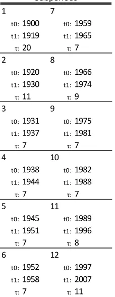
The panel data were created by taking averages or the values of variables in subperiods of
different lenght. The choice for different lengths is to take advantage of the data and coincide with
28
Table 3. Description of observations in data set.
Country Observations Missing observations
Starting year
Ending year
Argentina 108 0 1900 2007
The Bahamas 28 80 1975 2002
Belize 33 75 1975 2007
Bolivia 63 45 1945 2007
Brazil 108 0 1900 2007
Barbados 25 83 1975 1999
Chile 108 0 1900 2007
Colombia 108 0 1900 2007
Costa Rica 88 20 1920 2007
Cuba 76 32 1929 2004
Dominica 31 77 1977 2007
Dominican Republic 58 50 1950 2007
Ecuador 69 39 1939 2007
Grenada 28 80 1980 2007
Guatemala 88 20 1920 2007
Guyana 33 75 1975 2007
Honduras 88 20 1920 2007
Haiti 63 45 1945 2007
Jamaica 64 44 1913 2007
St. Kitts and Nevis 31 77 1977 2007
St. Lucia 28 80 1980 2007
Mexico 108 0 1900 2007
Nicaragua 88 20 1920 2007
Panama 63 45 1945 2007
Peru 108 0 1900 2007
Puerto Rico 52 56 1950 2001
Paraguay 69 39 1939 2007
El Salvador 88 20 1920 2007
Trinidad and Tobago 58 50 1950 2007
Uruguay 108 0 1900 2007
St. Vincent and the Grenadines 33 75 1975 2007
Venezuela 108 0 1900 2007
29
countries1 ly lppl pos countries1 ly lppl pos
arg mean 8.57 16.64 0.78 hnd mean 7.33 14.39 0.20
sd 0.36 0.60 0.20 sd 0.20 0.82 0.08
max 9.27 17.49 1.00 max 7.62 15.79 0.42
min 7.91 15.36 0.47 min 6.91 13.12 0.10
obs 108 108 108 obs 88 108 88
bhs mean 9.43 12.30 0.96 hti mean 6.88 15.11 0.09
sd 0.13 0.30 0.06 sd 0.15 0.54 0.03
max 9.54 12.72 1.00 max 7.17 16.09 0.20
min 9.05 11.66 0.80 min 6.61 14.26 0.04
obs 28 47 28 obs 63 108 63
blz mean 8.08 12.02 0.24 jam mean 7.94 14.18 0.27
sd 0.32 0.34 0.05 sd 0.41 0.43 0.05
max 8.57 12.65 0.33 max 8.33 14.80 0.39
min 7.64 11.45 0.17 min 6.41 13.49 0.16
obs 33 47 33 obs 64 108 64
bol mean 7.67 15.07 0.20 kna mean 8.13 10.70 0.26
sd 0.17 0.51 0.04 sd 0.47 0.06 0.09
max 7.96 16.07 0.33 max 8.74 10.83 0.39
min 7.36 14.34 0.14 min 7.33 10.60 0.14
obs 63 108 63 obs 31 47 31
bra mean 7.61 17.92 0.30 lca mean 7.62 11.72 0.15
sd 0.74 0.74 0.07 sd 0.30 0.20 0.04
max 8.76 19.06 0.43 max 7.92 12.03 0.20
min 6.52 16.70 0.20 min 7.03 11.38 0.10
obs 108 108 108 obs 28 47 28
brb mean 9.13 12.42 0.73 mex mean 8.02 17.33 0.44
sd 0.12 0.03 0.05 sd 0.57 0.71 0.07
max 9.33 12.47 0.81 max 8.94 18.47 0.64
min 8.90 12.35 0.63 min 7.21 16.43 0.29
obs 25 47 25 obs 108 108 108
chl mean 8.32 15.74 0.60 nic mean 7.45 14.19 0.23
sd 0.49 0.54 0.13 sd 0.30 0.83 0.09
max 9.48 16.63 1.00 max 8.12 15.54 0.40
min 7.58 14.91 0.37 min 6.91 13.08 0.07
obs 108 108 108 obs 88 108 88
col mean 7.77 16.43 0.34 pan mean 8.25 13.79 0.35
sd 0.57 0.74 0.05 sd 0.42 0.77 0.07
max 8.79 17.61 0.46 max 9.01 15.02 0.45
min 6.88 15.20 0.24 min 7.52 12.48 0.23
obs 108 108 108 obs 63 108 63
cri mean 8.01 13.88 0.37 per mean 7.70 16.06 0.32
sd 0.50 0.87 0.06 sd 0.55 0.66 0.06
max 8.89 15.31 0.47 max 8.49 17.17 0.47
min 7.26 12.60 0.24 min 6.71 15.15 0.21
obs 88 108 88 obs 108 108 108
cub mean 7.63 15.54 0.24 pri mean 8.76 14.58 0.62
sd 0.26 0.59 0.07 sd 0.57 0.43 0.23
max 8.02 16.23 0.43 max 9.66 15.19 1.00
min 6.88 14.32 0.15 min 7.67 13.77 0.29
obs 76 108 76 obs 52 108 52
dma mean 7.55 11.16 0.14 pry mean 7.72 14.30 0.23
sd 0.29 0.05 0.03 sd 0.31 0.79 0.07
max 7.90 11.22 0.19 max 8.16 15.63 0.44
min 6.93 11.02 0.08 min 7.31 12.99 0.15
30
Table 4. Description of observations in data set by country, where ly is the logarithm of GDP per capita, lppl is the logarithm of population and pos is the position of country with respect to the richest country.
countries1 ly lppl pos countries1 ly lppl pos
dom mean 7.63 14.74 0.18 slv mean 7.44 14.67 0.21
sd 0.41 0.92 0.04 sd 0.39 0.67 0.04
max 8.40 16.10 0.27 max 7.99 15.62 0.30
min 6.93 13.15 0.13 min 6.71 13.55 0.14
obs 58 108 58 obs 88 108 88
ecu mean 7.97 15.19 0.28 tto mean 9.08 13.40 0.78
sd 0.40 0.75 0.04 sd 0.41 0.53 0.16
max 8.50 16.41 0.36 max 9.95 14.10 1.00
min 7.17 14.15 0.21 min 8.21 12.50 0.46
obs 69 108 69 obs 58 108 58
grd mean 8.02 11.48 0.22 ury mean 8.40 14.56 0.66
sd 0.28 0.04 0.05 sd 0.37 0.39 0.17
max 8.35 11.54 0.30 max 9.14 15.02 1.00
min 7.50 11.39 0.14 min 7.70 13.73 0.40
obs 28 47 28 obs 108 108 108
gtm mean 7.81 15.09 0.31 vct mean 7.52 11.51 0.14
sd 0.31 0.75 0.11 sd 0.33 0.09 0.03
max 8.22 16.41 0.66 max 8.06 11.60 0.18
min 7.15 14.08 0.18 min 6.85 11.32 0.09
obs 88 108 88 obs 33 47 33
guy mean 8.04 13.50 0.23 ven mean 8.40 15.75 0.70
sd 0.11 0.07 0.03 sd 0.93 0.81 0.28
max 8.23 13.57 0.28 max 9.33 17.13 1.00
min 7.84 13.28 0.18 min 6.68 14.75 0.23
obs 33 47 33 obs 108 108 108
Total mean 7.96 14.68 0.38
sd 0.67 1.70 0.24
max 9.95 19.06 1.00
min 6.41 10.60 0.04
31
Table 5. Clubs in phase 1. ly is the logarithm of GDP per capita, lppl is the logarithm of population and pos is the position of country with respect to the richest country.
Mineral Agricultural
countries1 ly lppl pos countries1 ly lppl pos
chl mean 7.80 15.09 0.70 arg mean 8.17 15.86 1.00
sd 0.15 0.12 0.08 sd 0.13 0.28 0.01
max 8.13 15.29 1.00 max 8.38 16.29 1.00
min 7.58 14.91 0.59 min 7.91 15.36 0.95
obs 31 31 31 obs 31 31 31
mex mean 7.44 16.53 0.49 bra mean 6.75 17.02 0.24
sd 0.10 0.06 0.05 sd 0.16 0.19 0.03
max 7.60 16.66 0.64 max 7.05 17.33 0.30
min 7.21 16.43 0.38 min 6.52 16.70 0.20
obs 31 31 31 obs 31 31 31
per mean 6.98 15.31 0.31 col mean 7.09 15.53 0.34
sd 0.19 0.10 0.05 sd 0.11 0.21 0.03
max 7.39 15.50 0.43 max 7.32 15.88 0.46
min 6.71 15.15 0.25 min 6.88 15.20 0.30
obs 31 31 31 obs 31 31 31
ven mean 7.09 14.88 0.37 cri mean 7.40 12.88 0.42
sd 0.46 0.07 0.17 sd 0.05 0.15 0.04
max 8.14 15.01 0.80 max 7.50 13.12 0.47
min 6.68 14.75 0.23 min 7.33 12.60 0.36
obs 31 31 31 obs 11 31 11
cub mean 7.36 14.76 0.36
sd 0.06 0.26 0.02
max 7.40 15.16 0.38
min 7.32 14.32 0.35
obs 2 31 2
gtm mean 7.30 14.23 0.38
sd 0.10 0.09 0.02
max 7.48 14.39 0.41
min 7.15 14.08 0.36
obs 11 31 11
slv mean 6.89 13.87 0.25 hnd mean 7.20 13.43 0.34
sd 0.06 0.19 0.01 sd 0.10 0.19 0.03
max 6.97 14.18 0.27 max 7.35 13.76 0.37
min 6.82 13.55 0.22 min 7.04 13.12 0.28
obs 11 31 11 obs 11 31 11
ury mean 7.99 14.03 0.84 nic mean 7.22 13.28 0.35
sd 0.17 0.20 0.07 sd 0.12 0.11 0.03
max 8.37 14.35 1.00 max 7.47 13.43 0.40
min 7.70 13.73 0.67 min 7.08 13.08 0.30
32
Table 6. Clubs in phase 2. ly is the logarithm of GDP per capita, lppl is the logarithm of population and pos is the position of country with respect to the richest country.
Reactive Pasive
countries1 ly lppl pos countries1 ly lppl pos
arg mean 8.55 16.70 0.77 cub mean 7.50 15.61 0.27
sd 0.23 0.23 0.17 sd 0.23 0.27 0.06
max 9.03 17.06 1.00 max 7.79 16.05 0.43
min 8.17 16.31 0.52 min 6.88 15.18 0.18
obs 44 44 44 obs 44 44 44
bol mean 7.53 14.96 0.21 dom mean 7.22 14.75 0.15
sd 0.12 0.19 0.04 sd 0.18 0.43 0.02
max 7.79 15.35 0.33 max 7.63 15.45 0.20
min 7.36 14.70 0.16 min 6.93 14.08 0.13
obs 30 44 30 obs 25 44 25
bra mean 7.51 17.89 0.27 ecu mean 7.64 15.09 0.27
sd 0.38 0.35 0.04 sd 0.27 0.37 0.03
max 8.31 18.48 0.39 max 8.13 15.72 0.36
min 6.91 17.35 0.20 min 7.17 14.51 0.21
obs 44 44 44 obs 36 44 36
chl mean 8.27 15.70 0.58 gtm mean 7.71 14.98 0.34
sd 0.22 0.26 0.13 sd 0.21 0.38 0.13
max 8.64 16.14 0.81 max 8.10 15.61 0.66
min 7.73 15.30 0.42 min 7.21 14.41 0.22
obs 44 44 44 obs 44 44 44
col mean 7.71 16.38 0.33 hnd mean 7.20 14.30 0.20
sd 0.23 0.34 0.07 sd 0.14 0.36 0.07
max 8.19 16.97 0.46 max 7.40 14.92 0.42
min 7.28 15.90 0.24 min 6.91 13.79 0.14
obs 44 44 44 obs 44 44 44
cri mean 7.75 13.78 0.34 hti mean 6.91 15.03 0.12
sd 0.33 0.45 0.07 sd 0.07 0.22 0.03
max 8.40 14.51 0.46 max 7.01 15.44 0.20
min 7.26 13.14 0.24 min 6.76 14.71 0.08
obs 44 44 44 obs 30 44 30
mex mean 7.87 17.23 0.38 pan mean 7.87 13.76 0.30
sd 0.35 0.37 0.06 sd 0.28 0.34 0.06
max 8.52 17.87 0.49 max 8.35 14.33 0.41
min 7.22 16.68 0.29 min 7.52 13.17 0.23
obs 44 44 44 obs 30 44 30
nic mean 7.51 14.05 0.27 pri mean 8.28 14.60 0.44
sd 0.33 0.45 0.05 sd 0.40 0.17 0.14
max 8.08 14.81 0.40 max 8.90 14.89 0.69
min 6.91 13.44 0.20 min 7.67 14.28 0.29
obs 44 44 44 obs 25 44 25
per mean 7.81 15.95 0.36 slv mean 7.31 14.62 0.22
sd 0.34 0.30 0.06 sd 0.32 0.34 0.03
max 8.34 16.51 0.47 max 7.80 15.24 0.30
min 7.05 15.51 0.28 min 6.71 14.19 0.17
obs 44 44 44 obs 44 44 44
pry mean 7.44 14.26 0.23
sd 0.09 0.34 0.09
max 7.67 14.82 0.44
min 7.31 13.71 0.16
obs 36 44 36
ury mean 8.38 14.64 0.65 ven mean 8.79 15.58 0.96
sd 0.19 0.15 0.15 sd 0.47 0.43 0.08
max 8.59 14.85 0.94 max 9.28 16.32 1.00
min 7.92 14.37 0.46 min 7.87 15.02 0.74
33
Table 6. Clubs in phase 3. ly is the logarithm of GDP per capita, lppl is the logarithm of population and pos is the position of country with respect to the richest country.
Low Reformers High Reformers
countries1 ly lppl pos countries1 ly lppl pos
bra mean 8.55 18.82 0.38 arg mean 8.98 17.30 0.59
sd 0.09 0.17 0.03 sd 0.11 0.13 0.08
max 8.76 19.06 0.43 max 9.27 17.49 0.78
min 8.34 18.50 0.30 min 8.77 17.07 0.47
obs 33 33 33 obs 33 33 33
col mean 8.48 17.32 0.35 bol mean 7.80 15.73 0.18
sd 0.15 0.19 0.04 sd 0.09 0.21 0.03
max 8.79 17.61 0.44 max 7.96 16.07 0.24
min 8.19 16.99 0.31 min 7.64 15.38 0.14
obs 33 33 33 obs 33 33 33
cri mean 8.55 14.95 0.38 chl mean 8.88 16.41 0.54
sd 0.15 0.24 0.04 sd 0.34 0.15 0.13
max 8.89 15.31 0.46 max 9.48 16.63 0.73
min 8.35 14.53 0.31 min 8.37 16.16 0.37
obs 33 33 33 obs 33 33 33
cub mean 7.84 16.17 0.20 pan mean 8.59 14.71 0.39
sd 0.15 0.06 0.03 sd 0.17 0.20 0.03
max 8.02 16.23 0.24 max 9.01 15.02 0.45
min 7.52 16.06 0.15 min 8.32 14.36 0.31
obs 30 33 30 obs 33 33 33
dom mean 7.93 15.82 0.21 pri mean 9.21 15.08 0.79
sd 0.22 0.19 0.03 sd 0.24 0.08 0.16
max 8.40 16.10 0.27 max 9.66 15.19 1.00
min 7.66 15.48 0.17 min 8.85 14.91 0.61
obs 33 33 33 obs 27 33 27
ecu mean 8.32 16.13 0.30 pry mean 8.03 15.27 0.23
sd 0.08 0.20 0.03 sd 0.10 0.24 0.03
max 8.50 16.41 0.35 max 8.16 15.63 0.28
min 8.15 15.75 0.23 min 7.71 14.85 0.15
obs 33 33 33 obs 33 33 33
gtm mean 8.11 16.02 0.25 ury mean 8.83 14.95 0.50
sd 0.07 0.23 0.04 sd 0.15 0.05 0.06
max 8.22 16.41 0.32 max 9.14 15.02 0.62
min 7.98 15.64 0.18 min 8.60 14.86 0.40
obs 33 33 33 obs 33 33 33
hnd mean 7.54 15.41 0.14
sd 0.05 0.26 0.02
max 7.62 15.79 0.17
min 7.36 14.95 0.10
obs 33 33 33
mex mean 8.75 18.23 0.47
sd 0.10 0.18 0.04
max 8.94 18.47 0.55
min 8.55 17.89 0.36
obs 33 33 33
nic mean 7.46 15.24 0.14 slv mean 7.80 15.49 0.18
sd 0.28 0.21 0.06 sd 0.12 0.11 0.03
max 8.12 15.54 0.30 max 7.99 15.62 0.24
min 7.18 14.84 0.07 min 7.64 15.26 0.14
obs 33 33 33 obs 33 33 33
per mean 8.22 16.89 0.28 ven mean 9.11 16.80 0.68
sd 0.13 0.19 0.05 sd 0.11 0.23 0.16
max 8.49 17.17 0.40 max 9.33 17.13 1.00
min 7.96 16.53 0.21 min 8.85 16.36 0.43
34
Table 7. Description of subperiods of panel data. First line is the initial year, second line is the ending year, and the last line is
M
.
1 7
t0:1900 t0:1959
t1:1919 t1:1965 τ:20 τ:7
2 8
t0:1920 t0:1966 t1:1930 t1:1974
τ:11 τ:9
3 9
t0:1931 t0:1975
t1:1937 t1:1981
τ:7 τ:7
4 10
t0:1938 t0:1982 t1:1944 t1:1988
τ:7 τ:7
5 11
t0:1945 t0:1989 t1:1951 t1:1996
τ:7 τ:8
6 12
t0:1952 t0:1997
t1:1958 t1:2007 τ:7 τ:11