Benchmarking Methods in the Regulation of Electricity Distribution System Operators

Munich Personal RePEc Archive

Benchmarking Methods in the

Regulation of Electricity Distribution

System Operators

Janda, Karel and Krska, Stepan

University of Economics, Prague, Charles University in Prague

22 October 2014

Benchmarking Methods in the Regulation of

Electricity Distribution System Operators

∗

Karel Janda

and Stepan Krska

a

_{Charles University, Prague}

b

_{University of Economics, Prague}

October 22, 2014

Abstract

This paper examines the regulation of distribution system operators

(DSOs) focused the Czech electricity market. It presents an international

benchmarking study based on data of 15 regional DSOs including two Czech

operators. The study examines the application of yardstick methods using

data envelopment analysis (DEA) and stochastic frontier analysis (SFA).

Based on our results, we find that the cost efficiency of each of the Czech

DSOs is different, which indicates a suitability of introduction of individual

efficiency factors in the regulatory process.

∗_{The work on this paper was supported by the Czech Science Foundation (grant}

Keywords: Regulation, benchmarking, electricity.

JEL Codes: K23, L43, L49, L94

1

Introduction

The electricity distribution sector in the Czech Republic is dominated by three regional distribution system operators (DSOs). Their natural monopo-listic structure creates a need for regulation. Czech Energy Regulation Office (ERU) is applying incentive based revenue cap regulation, which is designed to motivate the incumbents to improve efficiency of their operation. The problem is that the firms are treated equally, regardless of the structure of the network that they control. The regulator employs only the general X factors that implicitly assume the firms to be similar. The equal treatment of DSOs is, however, very simplistic and if there are differences in cost effi-ciency among the operators, the less efficient operators are not incentivised to converge to the more cost efficient operators.

compa-rable firms. Another option is to model an efficient frontier of the compacompa-rable firms that serves as a yardstick (Kuosmanen et al., 2013). Given the Czech market structure, the option might be benchmarking of gas and electricity DSOs; however, there are significant differences between the sectors (storage, impact of the crisis, network specifics, etc.) and these may prove to be very difficult to control for. We believe that the suitable option, how to compute the efficiency of the incumbents, is to conduct a benchmarking analysis using the international dataset.

assumption that DSOs and TSOs should be benchmarked separately. Ku-osmanen et al. (2013) focused on the best practice benchmarking of DSOs. They compared DEA, SFA and StoNED (for more details, refer to Kuosma-nen et al., 2013) methods. StoNED methods are employed by Finnish regula-tor and combine advantages of DEA and SFA, however, they demand bigger datasets. Both Michael Pollitt and Timo Kuosmanen worked for national regulatory offices in England and Finland respectively, and they influenced the development of benchmarking for regulation in both countries.

As was mentioned above, a similar benchmarking study in the Czech Republic was not conducted yet. As far as we know, similar analysis was not conducted for other European countries that we examine either (namely Slovakia, Poland and Serbia). We follow papers that examined benchmark-ing methods in particular states. Farsi et al. (2005 and 2006) examined the panel of 59 Swiss distribution utilities using SFA estimated by gener-alised least squares, maximum likelihood and random effects models. Their analysis was facilitated by large dataset (around 380 observations) that sig-nificantly exceeds other studies. Agrell and Bogetoft (2011) supervised the final report on the use of benchmarking methods for the regulation of DSOs prepared for the Belgian regulator. They examined both gas and electricity DSOs and recommended DEA for the regulation. The general recommended variables were TOTEX (input), and number of connections, lines length and transformers (outputs).

regulation of electricity DSOs. According to Schweinsberg et al. (2011), regulators in 12 out of 27 EU members used methods of cost benchmarking in energy regulation.

Our study complements the already conducted studies and brings analysis of states that were outside of the field of interest of the researchers. We are, unfortunately, not allowed to disclose the computed efficiency scores for for-eign operators due to the contractual obligations; however, the international dataset brings the efficiency comparison among the companies and allows us to determine the efficiency scores for the Czech DSOs.

In the following sections, the yardstick methods used to measure the per-formance of DSOs and collected data are described. We adopt the DEA and SFA methods for benchmarking while taking into account the scope of the data available. The methods widely applied to the regulation of electricity markets are described and compared in the second section without formali-sation. The thorough formalisation of all methods and yardstick techniques (TFP, DEA, COLS, MOLS and SFA) would significantly exceed the recom-mended scope of the paper. This section encompasses description of the DEA and SFA methods and of the dataset. The purpose of the following sections is to outline the methodology and data used for a computation of the efficiency scores of DSOs.

2

Methodology

better fit the regulated decision making units (hereafter DMUs) and to mit-igate the information asymmetry. The terms DMU and firm are taken as interchangeable even though the firm may not be inappropriate for example in the case of benchmarking the public service companies, but in context of our study they are both relevant.

The most widely used techniques are the DEA methods combined with the stochastic frontier methods or methods based on the OLS regressions. In our study, the DEA models are preferred because of the limited scope of data while both the constant and variable return to scale DEA models are applied. In the literature, the DEA models are often complemented by a second stage OLS regression of efficiency parameters to control for other environmental characteristics that are typical of DSOs in the electricity sector. We checked the CRS DEA results and regressed coefficients on population density and the estimates confirmed the results of VRS DEA. Due to the size of dataset, we decided to apply both the CRS and VRS DEA specifications without second stage. The DEA models are supplemented with SFA, but we are aware of the limitations stemming from the size of the dataset.

2.1

Techniques

2.1.1 Data envelopment analysis

point on the frontier.

The DEA models can be both input and output oriented. The input-orientated DEA calculates how much the input quantities can be reduced without changing the output values. The output-orientated programmes how much the outputs can be expanded keeping the input quantities un-changed. The input-orientated DEA is generally appropriate for benchmark-ing of DSOs (e.g. Frontier Economics, 2012; Jamasb and Pollitt, 2003); moreover, the demand for distribution services is a derived demand, the in-cumbents cannot influence it and it has to be met because of the regulation (Jamasb and Pollitt, 2003). The models can be specified for constant or variable returns to scale (CRS, VRS respectively).

Firstly, we define the CRS input-based model. We will follow notation made by Coelli et al. (2005). Assume the dataset ofN firms containing data on K inputs and M outputs. They are represented by column vectors xi

and yi respectively. The input matrix X (K×N) and the output matrix Y

(M ×N) represent the data for all firms.

For each firm, we would like to obtain the efficiency score that is the maximum ratio of weighted outputs to weighted inputs for each DMU, such as u′_y

i/v′xi where u is a vector of output weights (M ×1) and v is a vector

max

u,v (

u′_y i

v′_xi) (1)

s.t. u

′_y j

v′_xj ≤1, j = 1, . . . , N

u, v ≥0.

The linear programming is solved for each DMU while the efficiency score must be less or equal to one. The problem of above mentioned programming problem is that it has infinite number of solutions (Coelli et al., 2005). If (˜u,v˜) are the solutions, then fora ǫR, (au, a˜ ˜v) are solutions as well; therefore, it is necessary to modify the model and impose a constraint of weighted inputs to equal one. Formally,

max

u,v (

u′_y i

v′_xi) (2)

s.t. v′_x i = 1,

u′_y j

v′_xj ≤1, j = 1, . . . , N

u, v ≥0.

min

θ,λ θ (3)

s.t. −yi+Y λ≥1

θxi−Xλ ≥0

λ≥0,

where θ is a scalar (equal to efficient score) and λ represents a N ×1 vector of constants. The problem (3) satisfies the assumption of efficiency score to be between zero and one while the DMU with θ = 1 is technically efficient. To obtain the efficient score for each DMU, the linear programming problem must be sold N times. In the model (3), the DMU i is compared to linear combination of other firms in the sample. It is obvious from the second condition that the output vectorxi is minimised while still remaining

in the feasible set of inputs that is bounded by the piece-wise linear isoquant determined by the firms included in the sample. The input vector xi is

radi-ally contracted on the isoquant (frontier) to the point (Xλ, Y λ). This point is a linear combination of the observed data points and given the constraints in the model (3), it is inside the feasible set.

the efficient frontier (Ozcan, 2008).

The problem of CRS DEA is that implicitly assumes that the firms are op-erating on the optimal scale. This assumption is violated in case of imperfect competition, regulations and other factors that restrict the firms to operate at optimal scale (Coelli et al., 2005). To get VRS DEA, the model (3) is modified by adding a convexity constraint Pλ= 1. If the CRS specification is applied to DMUs that are not operating on efficient scale, the technical efficiency is influenced by scale efficiencies. VRS DEA calculates technical efficiency less the scale efficiencies and the firms are compared against other DMUs with similar size. The VRS DEA model is defined

min

θ,λ θ (4)

s.t. −yi+Y λ≥1

θxi−Xλ ≥0

N1′_{λ= 1}

λ≥0,

where the N1 is aN ×1 vector of ones.

To find out the nature of the returns to scale, Coelli et al. (2005) recom-mends non-increasing returns to scale specification (NIRS) where the restric-tion N1′_{λ = 1 from (4) is replaced by restriction N1}′_{λ≤ 1. If the efficiency}

Using VRS DEA, the overall effect can be decomposed to technical ef-ficiency and scale efef-ficiency. Important advantage of DEA is that is does not suffer from problems with multicollinearity, because it is based on linear programming (Andor and Hesse, 2011; Went, 2007). Jensen (2005) showed that multicollinearity has little impact even on the results of SFA.

There are several rules of setting the minimal amount of DMUs for DEA to have good discriminatory power. The general rule of thumb is that the minimum number of DMUs should be at least twice the sum of inputs and outputs. Some authors recommend more prudent approaches - twice the multiple of inputs and outputs, three times the number of inputs and outputs and so forth (for more details, refer to Sarkis, 2007; or Cullinane and Wang, 2006).

2.1.2 Stochastic frontier analysis

In the previous section, we considered the non-parametric DEA to obtain efficiency measures. In this section, parametric estimation using SFA is con-sidered. The development of the SFA models is soundly described in the literature (e.g. Coelli et al., 2005; Greene, 2007). The main advantage of SFA compared to DEA is that it allows for statistical and functional form testing and separates noise and inefficiency. SFA requires specification of production (or cost) function requiring assumptions about production tech-nologies of DMUs.

We will consider costs as dependent variable in model similarly to DEA. The treatment of outputs and inputs will be therefore analogous.

DEA attributes the difference between the particular DMU and efficient firm to inefficiency. The estimation of deterministic production frontier could be conducted by methods based on OLS, but any deviation from determinis-tic efficient frontier is again assigned to inefficiency; however, the deviations might not be under control of the management and could be caused for ex-ample by measurement error or other source of statistical noise (Coelli et al., 2005). The stochastic frontier production function model was developed to overcome these problems.

There are several different expressions of the technology of the indus-try. The Cobb-Douglas and translog specifications are most frequently used in empirical applications. The Cobb-Douglas form is more restrictive in as-sumptions but usually preferred over translog specification for benchmarking of DSOs with smaller samples. SFA is estimated using the maximum likeli-hood estimation techniques.

We start with a model for cross-sectional data and follow notational sys-tem from Coelli et al. (2005). The stochastic production function model was simultaneously proposed by Aigner et al. (1977) and Meeusen and van Den Broeck (1977) in form

lnqi =x′iβ+vi−ui, (5)

whereqi is dependent variable of i-th firm (input in case of cost frontier);

xi is aK×1 vector of logarithms of explanatory variables (outputs in case of

error accounting for statistical noise; and ui is non-negative random variable

associated with inefficiency. The statistical noise is caused by measurement error, omission of relevant variables and it can arise from approximation of errors related to the functional form of the production (or cost) function. The model is bounded from above by stochastic variable exp(x′

iβ+vi) that

gives the model its name.

Let us further assume production function. The SFA frontier can be illustrated graphically. Taking the Cobb-Douglas stochastic frontier (5) of the production function with single dependent (output) and single explanatory (input) variables, we have

lnqi =β0+β1lnxi+vi−ui. (6)

If we rearrange the equation (6), we get

qi = exp(β0+β1lnxi)×exp(vi)×exp(−ui), (7)

where exp(β0 +β1lnxi) is deterministic component; exp(vi) represents

noise; and exp(−ui) is inefficiency term. Assume the deterministic frontier

to reflect the decreasing returns to scale. Further assume two firms, firm A and firm B. Firm A produces output qA using input xA, firm B uses xB

to produce qB. If the both firms are effective, i.e. there are no inefficiency

effects (uA = 0 ∧ uB = 0), the production functions are

q∗

Further assume the noise effect for firm A to be positive (vA > 0) and

for firm B to be negative (vB <0), and deterministic frontier qi = exp(β0+

β1lnxi).

The position of the firm with respect to the deterministic frontier depends on the magnitudes of noise and inefficiency effects.

Most of the frontier analyses are aimed at prediction of inefficiencies. The technical efficiency is defined as ratio of observed output to the SFA output

T Ei =

qi

exp(x′ iβ)

= exp(−ui). (9)

The value of technical efficiency is between zero and one and it represents the ratio of the company’s output to the output that could be produced by fully efficient firm using the same vector of inputs. A drawback of SFA is that even if there are no statistical errors, some may be wrongly regarded as noise (Jamasb and Pollitt, 2003).

The estimation of the SFA parameters is more complicated due to two random terms included in the right hand side of the equation (5); there-fore, some assumption concerning these terms should be made. Assume vi

are random variables that are assumed to be independently and identically distributed (i.i.d), vi ∼ N(0, σv2) and independent of ui; ui are non-negative

random variables assumed to be i.i.d,ui ∼ |N(0, σu2)|(Coelli, 1996b). Aigner

et al. (1977) obtained maximum likelihood estimators under these assump-tions and parameterised the log-likelihood function for half-normal model. Assume σ2 _{= σ}2

v +σu2 and λ2 = σ2

u

σ2

v

for σ2

v ≥ 0. There are no inefficiency

effects if λ2 _{= 0 and the deviations from frontier are due to statistical noise.}

The ui is homoscedastic with constant mean and uncorrelated; the vi is

homoscedastic, with zero mean and uncorrelated (similar properties to the noise of the classical linear regression model). The OLS model cannot be used for estimation, because the intercept is biased downwards. Coelli et al. (2005) suggest the use of maximum likelihood method for better asymptotic properties in comparison with adjusted OLS models (e.g. COLS, MOLS).

The general model (5) from Aigner et al. (1977) can be extended to panel data. The model is expressed as (Battese and Coelli, 1992)

lnqi,t =x′i,tβ+vi,t −ui,t, (10)

where time factor t is added. Statistical noise is assumed to be i.i.d,

vi ∼ N(0, σv2) and independent of inefficiency term. The inefficiency term

may vary over time

ui,t =uiexp[−η(t−T)], (11)

whereui are random non-negative variables assumed to be i.i.d. as

trun-cations at zero of N(µ, σ2

u) distribution; η parameter to be estimated; and

the panel dataset does not have to be balanced.

Using parameterisation of Battese and Corra (1977), we introduce γ :=

σ2

u/(σv2+σu2) that represents the share of technical efficiency in error term. If

γ = 0, all deviations from the frontier are attributed to statistical noise; on the other hand if γ = 1, all deviations are caused by inefficiency. For more details, refer to Battese and Corra (1977), Battese and Coelli (1992), Coelli (1996a), Coelli (1996b) and Coelli et al. (2005).

total expenditures), the equation (10) is adjusted (Coelli, 1996b)

lnqi,t =x′i,tβ+vi,t +ui,t, (12)

all other factors keeping the same. In case the cost function in equation (12) is considered, the ui,t term defines the cost inefficiency of the firm, i.e.

the distance of the firm from the cost frontier. Some authors recommend translog form for cost function specification (e.g. Coelli et al., 2005; Agrell and Bogetoft, 2011). We considered the option, but due to the limited dataset and loss of degrees of freedom, we applied log-linear functional form. In case of larger dataset, we would test both options and compare results.

2.2

Data description

Our benchmarking study is based on data of the electricity DSOs. We focus on the unbundled regional DSOs with more than 100,000 customers. The inclusion of smaller DSOs would increase the size of the dataset, but the differences would have significant impact on the computed efficiency scores. We complemented the Czech DSOs with companies from other European countries.

compa-nies. The financial statements are publicly accessible in the Czech Republic, but it is very uncommon in the international comparison. Sometimes con-solidated data for particular energy groups are available, but they do not include detailed data. During the data collection, we had to sign several con-tracts and declarations on oath and we had to pledge to anonymise the data. Thus we cannot mention companies’ names and we can only state descriptive statistics of the dataset.

We obtained data of 15 DSOs from the Czech Republic, Slovakia, Poland, Hungary and Serbia. The data are from financial statements, annual reports, reports to the regulatory authorities, websites and mostly supplemented by data provided directly by the companies. All companies are unbundled and operating on the regional basis. We sought data from the Austrian DSOs and contacted all 11 DSOs distributing energy to more than 100,000 customers, but none of them provided us demanded data.

The only data we were able to obtain directly without help were the data of Czech DSOs. There are three regional DSOs in the Czech Republic, but we can use only two of them for our study, because the company E.On Distribuce, a.s. did not provide us with financial data that would be usable for our analysis. The published financial statements are consolidated for distribution of both gas and electricity and it was no possible to obtain the separated cost data; therefore, only ˇCEZ Distribuce, a.s. and PREdistribuce, a.s. are included. We obtained the data from annual reports, distribution quality reports and websites. The data and documents are available online at websites of the companies.

Jamasb and Pollitt, 2003; Haney and Pollitt, 2009; Kuosmanen et al., 2013; Shuttleworth, 2005) and practical application (e.g. EY, 2013; Frontier Eco-nomics, 2010; Frontier EcoEco-nomics, 2012; Schweinsberg et al., 2011).

The data are analysed using two methods, therefore, they are adjusted accordingly. For DEA, cross-sectional data for 2012 are used. We sought most up to date data and endeavour to obtain complete dataset of 2012. Data of some firms we were able to obtain from 2010 to 2012 and the panel is used for SFA. The balanced panel is not necessary for SFA and we utilise this characteristic.

The inputs (costs) are represented in monetary values. They are adjusted for inflation using annual growth rate and denominated in euro with 2012 as a base year. The exchange rates were used as at the end of individual years, because the costs were taken mostly from financial statements that consider exchange rate at the year end.

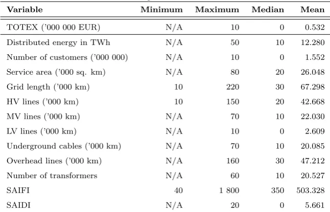
The summary statistics over the data are depicted in Table 1. The data are rounded to comply with the rules of DSOs and to guarantee anonymi-sation. To anonymise the data, values for minimum, maximum and median are rounded to the nearest ten. Most of the minimum values have to be anonymised with designation “N/A”, because the minimum values would be attributable to single company. We are aware of the low information value, but we are limited by the signed contracts and declarations on oath.

Table 1: Summary statistics over dataset

Variable Minimum Maximum Median Mean

TOTEX (’000 000 EUR) N/A 10 0 0.532

Distributed energy in TWh N/A 50 10 12.280

Number of customers (’000 000) N/A 10 0 1.552

Service area (’000 sq. km) N/A 80 20 26.048

Grid length (’000 km) 10 220 30 67.298

HV lines (’000 km) 10 150 20 42.668

MV lines (’000 km) N/A 70 10 22.030

LV lines (’000 km) N/A 10 0 2.609

Underground cables (’000 km) N/A 70 10 20.085

Overhead lines (’000 km) N/A 160 30 47.212

Number of transformers N/A 60 10 20.527

SAIFI 40 1 800 350 503.328

SAIDI N/A 20 0 5.661

2.2.1 Input variables

DEA can be used for estimation of multiple inputs and outputs while SFA requires specification of the cost function (or production function) with single dependent variable. The single input model utilises comparability of the results of both methods.

We use input variable (dependent variable in case of SFA) in monetary terms in form of total expenditures (TOTEX). We obtained capital expen-ditures, however, the investments in distribution networks are cyclical and given the scope of analysis (panel data for SFA), the use of CAPEX would require long panel data or adjustments. Therefore, we prefer total costs to be benchmarked.

using only the exchange rates, because the capital expenditures comprise mostly of materials traded in euro and the direct labour costs form a minor share of TOTEX of the utilities. We do not consider the transformation using purchasing power parity to be convenient. In other studies, we did not observe similar adjustments.

In some of the models, the total costs are weighted by distributed energy and represents costs of unit of distributed energy.

2.2.2 Output variables

Our models are based on the output (dependent) variables we obtained. The selection is based on the literature and practice of regulators. We consider these variables as major cost drivers. Except for quality parameters (SAIFI and SAIDI), the parameters are assumed to be non-discretionary or to limited extent manageable by the incumbents. The output variables are

• distributed energy in MWh,

• number of clients (grid connection points),

• service area (sq. km),

• grid length (area),

• low voltage lines (km);

• medium voltage lines (km);

• high voltage lines (km);

• length of overhead lines (km),

• number of transformers,

• quality parameters - SAIDI, SAIFI.

These are the general variables used for estimation. The specifications of models based on these data are described in the following sections.

2.3

Estimated models

2.3.1 Estimated DEA models

The input (dependent) variable of all models is represented by total ex-penditures. The explanatory (output) variables differ. For DEA, we use four output variables for analyses and consider methods with both CRS and VRS. We use a mean normalisation of data to correct for imbalances in data magnitudes. The normalisation is recommended by Sarkis (2007) to address possible scaling effects of the software. The DEAP does not indicate any problems, but we decided to normalise the data for the sake of accuracy. The normalisation is defined

¯

Ai = N

X

n=1

Ani

N , (13)

where ¯Ai is the mean for i-th output or input; N is a number of DMUs;

and Ani is a value of particular input (output) of n-th DMU.

The outputs for first DEA model (DEA1) are:

• (2) grid length (km) weighted by distributed energy (MWh),

• (3) transformers (count) weighted by distributed energy (MWh),

• and (4) inverse value of interruption duration (min) per MWh.

The interruption duration is computed from the SAIDI coefficient, which is multiplied by number of customers and weighted by distributed energy. The value is inverted, because the lower the interruption duration is, the more costly the grid maintenance is assumed to be. The weighting of parameters is used to address to multicollinearity of output variables. As mentioned above, multicollinearity is not a problem for DEA, but high correlations among variables may decrease the descriptive power. The weighting is also preferred in the practical usage of DEA (e.g. benchmarking of DSOs in Norway).

For the second DEA model (DEA2), the outputs are

• (1) area of the distribution network (sq. km)

• (2) grid length (km) weighted by distributed energy (MWh)

• (3) transformers (count) weighted by distributed energy (MWh),

• and (4) share of underground cables (%).

2.3.2 Estimated stochastic frontier models

In regulatory practice, the parameters used for SFA are similar to DEA and both methods are compared. We estimate three models. Two of them are using similar variables as our DEA model.

We use unbalanced panel specification of the SFA cost model. We use a log-linear model specification. This specification employs a Cobb-Douglas cost functional form and it is linear in log of the variables. The log-linear model specification for SFA1 is

lnT OT EXi,t =β0+β1lnAREAi,t+β2N ET Wi,t (14)

+β3T RANi,t+β4IN T Ei,t+ui,t+vi,t,

where dependent variable T OT EX are total expenditures expressed in euro weighted by distributed energy; explanatory variables (AREA, N ET W,

T RAN and IN T E) are similar to outputs in DEA1; u is inefficiency term;

v is noise term; βs are unknown parameters to be estimated; iǫ{1, ..,15} is the coefficient for particular companies; and tǫ{1,2,3} is a time parameter for 2010-2012 years. The variable for interruptions is not inverted, because inversion is not necessary in case of SFA. The variables are not weighted by MWh as in the case of DEA, because the values must be greater than one due to the logarithmic form. For SFA, the data were scaled by 10 TWh instead of GWh of delivered energy.

The third SFA model, SFA3, we defined as unweighted. We are aware of the high correlation coefficient between distributed energy and number of transformers (0.87); however, Jensen (2005) showed that multicollinearity has little impact even on results of SFA and therefore we decided to include also unscaled model. The selection of explanatory variables was based similarly to previous models on regulatory practice. The model is defined

lnT OT EXu

i,t =β0+β1lnDIST +β2CABL (15)

+β3T RANi,tu +ui,t+vi,t,

where dependent variable T OT EXu _{represents unscaled total costs;}

ex-planatory variables are DIST (represent distributed energy), CABL (al-ready defined cables’ share), andT RANu _{(unscaled number of transformers)}

other variables keeping similar to two previous models.

An important advantage of SFA is the possibility of statistical testing. The significance of estimated parameters (βs) can be tested comparing the computed t-statistics with critical values from ordinary statistical tables. In addition to testing of the parameters of cost function, the existence of inefficiency effects can be tested. SFA requires a priori assumption about the distribution of inefficiency term. There two options, either to conduct simple z-test or likelihood-ratio test (LR test). Coelli et al. (2005) suggest using of one sided LR test, because the z-test has a poor performance for small samples. The Frontier automatically gives values of one-sided likelihood ratio test. The null hypopaper is inexistence of inefficiency effects, i.e. H0 :

truncated-normal model. The statistic value of the LR test of the half-truncated-normal model is to be compared with χ2

1−2α(x) distribution whereα is a level of statistical

significance and x refers to number of restrictions. The critical value for the truncated-normal model can be obtained from Table 1 in Kodde and Palm (1986).

The appropriateness of the truncated-normal model over the half-normal model can be also tested using values computed by the Frontier. The LR test statistic is

λ =−2 [lnL(H0)−lnL(H1)], (16)

where lnL(H0) and lnL(H1) are statistics for log-likelihood values

re-ported for half-normal and truncated-normal models. The null is H0 : µ= 0

against alternative H1 : µ 6= 0. The value of the test statistic (16) is to

be compared with χ2

1−α(x) where α is a level of statistical significance andx

refers to number of iterations of half-normal model.

3

Results

3.1

DEA models

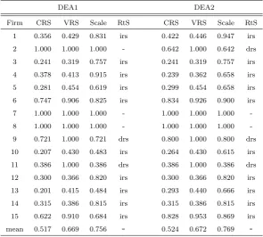
As described in the previous section, there are two specifications of the DEA models to be tested. We apply input-based VRS specification of the models while DEAP presents also efficiency scores for the CRS specification. The DEAP in addition computes values for NIRS DEA to compute the nature of the returns to scale. The technical efficiency scores are depicted in Table 2, which contains values of both DEA models and encompasses the efficiency scores for the CRS and VRS specifications, scale effects, and nature of the returns to scale (abbreviation irs is for increasing returns to scale, drs for decreasing returns to scale and dash for constant return to scale).

Given the CRS specification, we assume that the firms are operating on the same scale. Since the dataset is comprised of companies of diverse size and from different countries, we consider the VRS specification to be more appropriate. If we use the CRS model, the technical efficiency scores might be confounded by scale efficiencies. The scale efficiency is defined by computing both CRS and VRS models, and then decomposing the efficiency scores obtained by CRS DEA to scale and pure technical inefficiency. If the efficiency scores obtained from the CRS and VRS models differ, then it indicates the existence of scale inefficiency. The technical efficiency score of the CRS specification is equal to multiple of the VRS efficiency score and scale efficiency score.

Table 2: Summary of DEA efficiency scores

DEA1 DEA2

Firm CRS VRS Scale RtS CRS VRS Scale RtS

1 0.356 0.429 0.831 irs 0.422 0.446 0.947 irs

2 1.000 1.000 1.000 - 0.642 1.000 0.642 drs

3 0.241 0.319 0.757 irs 0.241 0.319 0.757 irs

4 0.378 0.413 0.915 irs 0.239 0.362 0.658 irs

5 0.281 0.454 0.619 irs 0.299 0.454 0.658 irs

6 0.747 0.906 0.825 irs 0.834 0.926 0.900 irs

7 1.000 1.000 1.000 - 1.000 1.000 1.000

-8 1.000 1.000 1.000 - 1.000 1.000 1.000

-9 0.721 1.000 0.721 drs 0.800 1.000 0.800 drs

10 0.207 0.430 0.483 irs 0.264 0.430 0.615 irs

11 0.386 1.000 0.386 drs 0.386 1.000 0.386 drs

12 0.300 0.366 0.820 irs 0.300 0.366 0.820 irs

13 0.201 0.415 0.484 irs 0.293 0.440 0.666 irs

14 0.315 0.386 0.815 irs 0.315 0.386 0.815 irs

15 0.622 0.910 0.684 irs 0.828 0.953 0.869 irs

mean 0.517 0.669 0.756 - 0.524 0.672 0.769

-to five and the mean efficiency increases in both cases. Most of the firms exhibit non-constant returns to scale, but there are still significant differences among the benchmarked firms. The problem of VRS specification is that the validity depends on the size of the sample and VRS DEA tends to overstate the efficiency scores (Jamasb and Pollitt, 2003). The various categories of the firms should be sufficiently represented in the sample that is, however, limited in our case due to the small sample of firms.

3.2

SFA models

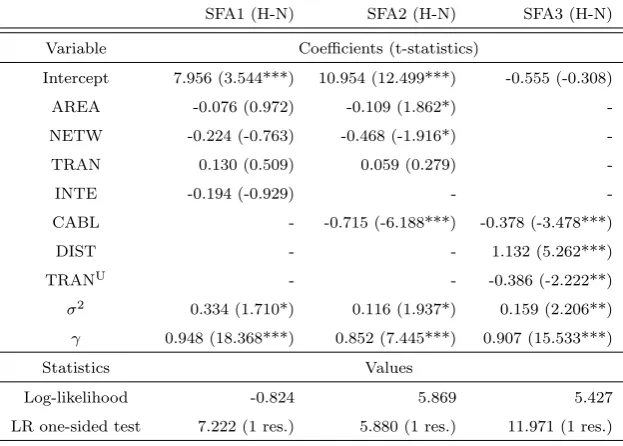
The SFA models are computed using programme Frontier. All the SFA models are defined in Cobb-Douglas log-linear specification and modelled as cost functions. The dataset in unbalanced for 15 firms with 28 observations. Both truncated-normal and half normal distributions of the inefficiency term are considered and tested. Summary statistics are reported in Table 3 for the half-normal and Table 4 for the truncated-normal models. The values of estimated coefficients are reported in columns while in parentheses the t-statistics are depicted. The level of significance of the estimates is represented by stars in parentheses. For LR test, the number of restrictions is depicted in parentheses. The nature of the variables is described in previous section in detail.

Table 3: Summary of SFA parameters with half-normal distribution of inef-ficiency term

SFA1 (H-N) SFA2 (H-N) SFA3 (H-N)

Variable Coefficients (t-statistics)

Intercept 7.956 (3.544***) 10.954 (12.499***) -0.555 (-0.308)

AREA -0.076 (0.972) -0.109 (1.862*)

-NETW -0.224 (-0.763) -0.468 (-1.916*)

-TRAN 0.130 (0.509) 0.059 (0.279)

-INTE -0.194 (-0.929) -

-CABL - -0.715 (-6.188***) -0.378 (-3.478***)

DIST - - 1.132 (5.262***)

TRANU _{- - -0.386 (-2.222**)}

σ2 _{0.334 (1.710*) 0.116 (1.937*) 0.159 (2.206**)}

γ 0.948 (18.368***) 0.852 (7.445***) 0.907 (15.533***)

Statistics Values

Log-likelihood -0.824 5.869 5.427

LR one-sided test 7.222 (1 res.) 5.880 (1 res.) 11.971 (1 res.)

Statistical significance: * refers to 10%, ** refers to 5%, and *** refers to 1% significance.

vari-ables is significant at the 10% level. The value of γ indicates that 95% of the variation in error term is attributable to technical efficiency and only 5% to statistical noise. In the SFA2 model, two coefficients are weakly significant at the 10% level of significance, one is significant at the 1% level and remaining coefficient at variable T RAN is not statistically significant at the 10% level. The second model exhibits lowest variance and only 15% of the variation in error term is attributable to noise. In the third model, all coefficients are significant at least at the 5% level. The model has lower variance than model SFA1 and around 9% of the error term is attributable to statistical noise. To test the existence of inefficiency effects withH0 : λ= 0, the values of LR test

are compared with χ2

0.9(1) = 2.706. Since the values reported for the models

exceed the critical value, we can reject the null hypopaper of no inefficiency effects at the 5% level of significance.

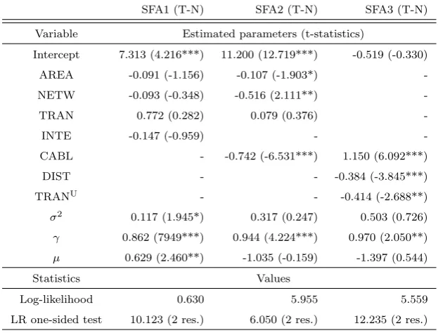
Table 4: Summary of SFA parameters with truncated-normal distribution of inefficiency term

SFA1 (T-N) SFA2 (T-N) SFA3 (T-N)

Variable Estimated parameters (t-statistics)

Intercept 7.313 (4.216***) 11.200 (12.719***) -0.519 (-0.330)

AREA -0.091 (-1.156) -0.107 (-1.903*)

-NETW -0.093 (-0.348) -0.516 (2.111**)

-TRAN 0.772 (0.282) 0.079 (0.376)

-INTE -0.147 (-0.959) -

-CABL - -0.742 (-6.531***) 1.150 (6.092***)

DIST - - -0.384 (-3.845***)

TRANU _{- - -0.414 (-2.688**)}

σ2 _{0.117 (1.945*) 0.317 (0.247) 0.503 (0.726)}

γ 0.862 (7949***) 0.944 (4.224***) 0.970 (2.050**)

µ 0.629 (2.460**) -1.035 (-0.159) -1.397 (0.544)

Statistics Values

Log-likelihood 0.630 5.955 5.559

LR one-sided test 10.123 (2 res.) 6.050 (2 res.) 12.235 (2 res.)

Statistical significance: * refers to 10%, ** refers to 5%, and *** refers to 1% significance.

The negative signs of estimates and high coefficients at intercepts may seem to be difficult to interpret. Initially, we were surprised with the signs, but the results are in line with previous research (e.g. Jamasb and Pollitt, 2003). The negative signs can be interpreted by scale effects and increasing returns to scale. The high values of γ indicates that most of the error term is attributable to inefficiency. The low values would indicate wrong specifi-cation of the model and on the contrary very high values approaching 100% would need to be cautiously treated, because absence of noise is not likely to occur especially in the cross-country comparison.

The values of LR test are compared with critical values obtained from Table 1 in Kodde and Palm (1986). Taking the 5% level of significance, the critical value is equal to 5.138. The reported values exceed the critical value thus we can reject the null at the 5% level of significance.

In the last step, we test the appropriateness of the use of the truncated-normal over the half-truncated-normal distribution of the inefficiency term. The test statistic is defined in expression (16). The null hypopaper is that the half-normal model is adequate, H0 : µ= 0, against alternative H1 : µ6= 0. The

computed statistics of the test give

• λSF A1 =−2[7.222−10.123] = 5.802,

• λSF A2 =−2[5.880−6.050] = 0.34,

• λSF A23 =−2[11.971−12.235] = 0.528,

and the critical value at the 5% level of significance is χ2

0.95(1) = 3.841;

therefore, we have to reject the null in case of first model and we cannot reject the null for SFA2 and SFA3 at the 5% level of significance.

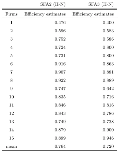
Table 5: Summary of SFA cost efficiency estimates

SFA2 (H-N) SFA3 (H-N)

Firms Efficiency estimates Efficiency estimates

1 0.476 0.400

2 0.596 0.583

3 0.752 0.586

4 0.724 0.800

5 0.731 0.800

6 0.916 0.863

7 0.907 0.881

8 0.922 0.889

9 0.747 0.642

10 0.835 0.716

11 0.846 0.816

12 0.843 0.786

13 0.749 0.728

14 0.879 0.900

15 0.899 0.946

mean 0.764 0.720

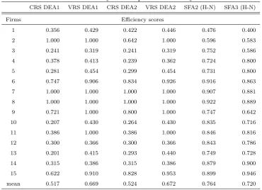
3.3

Summary of results

In this section, results from preferred models are described and summarised. The results are depicted in Table 6. We include the CRS and VRS efficiency scores obtained by both the DEA models and efficiency scores of the SFA2 and SFA3 models. The SFA models are specified with half-normal distribu-tion of inefficiency term.

results is caused by differences in nature of the methods.

In the regulatory benchmarking practice, the results from different meth-ods are considered. The results are usually weighted and final efficiency scores are based on scaling. The weighted sum of efficiency scores helps to deal with particularities of different models. In the current 2014-2018 regu-latory period in Austria, the results from two DEAs and MOLS are scaled and used.

The Austrian energy regulatory office employs CRS DEA. The CRS speci-fication is chosen under an assumption that possible scale inefficiencies would be solved by mergers or joint ventures within the market (Frontier Economics, 2012). German regulator applies CRS DEA and SFA and takes into the ac-count results from both methods; however, benchmarking in Austria and Germany is based on the data of national DSOs and since our study is based on international dataset, we believe that the VRS specification is also valid. Considering the practice of regulators, we include both specifications in our final comparison.

Table 6: Summary of computed efficiency scores

CRS DEA1 VRS DEA1 CRS DEA2 VRS DEA2 SFA2 (H-N) SFA3 (H-N)

Firms Efficiency scores

1 0.356 0.429 0.422 0.446 0.476 0.400

2 1.000 1.000 0.642 1.000 0.596 0.583

3 0.241 0.319 0.241 0.319 0.752 0.586

4 0.378 0.413 0.239 0.362 0.724 0.800

5 0.281 0.454 0.299 0.454 0.731 0.800

6 0.747 0.906 0.834 0.926 0.916 0.863

7 1.000 1.000 1.000 1.000 0.907 0.881

8 1.000 1.000 1.000 1.000 0.922 0.889

9 0.721 1.000 0.800 1.000 0.747 0.642

10 0.207 0.430 0.264 0.430 0.835 0.716

11 0.386 1.000 0.386 1.000 0.846 0.816

12 0.300 0.366 0.300 0.366 0.843 0.786

13 0.201 0.415 0.293 0.440 0.749 0.728

14 0.315 0.386 0.315 0.386 0.879 0.900

15 0.622 0.910 0.828 0.953 0.899 0.946

mean 0.517 0.669 0.524 0.672 0.764 0.720

PREdistribuce, a.s. are included in the sample. The efficiency scores of city operators are on average similar to efficiency scores of DSOs operating larger regions with lower population densities; therefore, the better performance of PREdistribuce, a.s. cannot be simply attributable to the smaller area the company is distributing the electrical energy on.

3.4

Policy implications

The energy sector in the Czech Republic can be considered as infant. There are still discussions about the setting of the regulatory parameters. The obstacles were shown during the discussion process preceding the fourth reg-ulatory period of the regulation of gas sector in the Czech Republic. There were problems with definitions of amortisation and depreciation, investments, etc. There can be problems inherited from the past that can be beyond con-trol of the managements. The current regulatory setting does not generate sufficient incentives for development. In the current regulatory formula, the quality and development parameters are not sufficiently emphasised. Addi-tional parameters promoting development of the grid should be encompassed in the regulation and also considered in the setting of benchmarking meth-ods. DSOs should be more incentivised to invest in new technologies. The development of smart grids, smart metering and more effective methods of management of renewable energy sources in the Czech Republic should be more accented in the future.

rela-tive performance in comparison with peers and we consider it as an auxiliary tool for regulation. We are aware of possible shortcomings of the methods that are also endorsed by the use of international dataset.

Setting the efficient companies lying on the frontier (DEA), or the most efficient companies (in case of SFA), as a yardstick would be too restrictive. We would propose to set the objective efficiency value as a mean (or median) efficiency score. Similar methodology is applied by the Norwegian regulator (Frontier Economics, 2012). The companies operating above the mean (or median respectively) are considered as effective and allocated only general X factor. The companies operating below would be incentivised by the indi-vidual X factors to improve efficiency of their performance. Another method would be to set the floor similarly as the German regulator. If the company is below some artificial value (in Germany 0.6), it would be treated as having this minimum value.

We realise that international benchmarking is problematic. Similarly, the size of our dataset confines the representativeness of our results. The use of benchmarking would be the tool which suitability was proven in regulatory practice if the Czech regulator seeks to set individual X factors in the future; moreover, the Czech regulator is able to acquire the data of the EU regulated companies and conduct comprehensive analysis with larger dataset. We were informed by the representatives of ERU that the data are exchanged by the EU regulators within the Agency for Cooperation of Energy Regulators on regular basis.

company’s score was only in one case above median value. The company PREdistribuce, a.s. obtained better scores and in three DEA models it was a frontier firm, but in both SFA models it obtained efficiency scores below mean and median. The Czech DSOs scored worse than comparable firms from abroad that indicates improvement potential. There are only three companies dominating the Czech market and the regulator can hardly dis-pose of complete information about the firms. There is a risk of regulatory capture. We mentioned all the regulatory constraints defined by Laffont and Tirole (1996) and the political risk can also be an issue. The regulator is established as independent, but two out of three incumbents are still con-trolled by the state. The inefficient operation is indicated in international comparison by fees for distribution included in the price of electricity. The Slovak regulator conducted analysis of fees for electricity distribution in the selected EU countries (URSO, 2011). The examined countries were Slovakia, the Czech Republic, Poland, Hungary, Germany and Austria. The fee was in the Czech Republic on average (average fee for all voltage lines) higher than in Slovakia, Poland and Hungary and comparable with Austria. In Ger-many, the average fee was highest due to the by far largest fee imposed on the households to bear significant amount of cost that skewed the average value.

of the incumbents and would be complicated due to the above mentioned constraints the regulator has to always face. We showed in our analysis that the efficiency between the Czech DSOs markedly differ and that their operation is less efficient in comparison to foreign firms. The inclusion of only general efficiency factor in the regulatory formula is therefore not sufficient to improve their operation. We are aware of the fact that a more comprehensive dataset is necessary for precise setting of the individual X factors and we are aware of problems stemming from the limited size of the dataset we used. The larger dataset would increase the descriptive power of our results, however, the minimum criteria for DEA were fulfilled. Similarly, the more comprehensive dataset would improve the results of SFA. We recommend ERU to conduct similar benchmarking analysis with a larger dataset. The results should be used for the adjustment of general X factor and primarily to introduce the individual X factors that ERU was not able to incorporate in regulatory formula of the current third regulatory period.

4

Conclusion

controlling certain regions. Due to the liberalisation that was institution-alised at the EU level, the companies also share similar structure as they have to be unbundled from other activities.

Our main research question was to evaluate the use of benchmarking methods for the regulation of DSOs. Benchmarking of the incumbents would facilitate introduction of the individual X factors corresponding to efficiency of particular incumbents. Similar analysis has not been conducted yet, as far as we know.

We collected a dataset comprising of 15 unbundled companies from the Czech Republic, Slovakia, Poland, Hungary and Serbia. The data gathering was complicated due to confidentiality. We are not allowed to disclose the data and the names of the foreign companies, however, it does not affect representativeness of our paper as we sought to find the efficiency scores for the Czech DSOs. The dataset comprises companies that are similar to the Czech DSOs in terms of area and population served. The data of the Czech companies are public and therefore we can present our results. We were only able to use the data for ˇCEZ Distribuce, a.s. and PREdistribuce, a.s. The financial statements for E.On Distribuce, a.s. are consolidated for distribution of electricity and gas and the company refused to provide us with unconsolidated cost data.

inflation using annual growth rate and denominated in euro with 2012 as a base year. The total expenditures were taken as input (dependent variable) and the outputs (dependent variables) were based on grid parameters and outputs. The selection of parameters was based on theory and practical ex-perience of regulators applying benchmarking of DSOs. The weighting of outputs was applied to address high correlation among the output variables. The results of our analysis showed significant differences among efficiency scores of both Czech companies. The efficiency scores of ˇCEZ Distribuce, a.s. were below mean efficiency in all six models conducted while only in one case the efficiency score was above median. The company PREdistribuce, a.s. obtained higher scores. In case of three out of four DEA models, it was a frontier firm; however, in SFA models the efficiency was below mean and median. Our models confirmed varied efficiency of Czech DSOs that should be addressed in the forthcoming fourth regulatory period. We believe that individual efficiency factors should be implemented to control for these differences.

Benchmarking serves as a suitable tool for assessment of the cost efficiency of the Czech operators in international comparison. The results showed that the Czech DSOs are in the international comparison among the less efficient companies. This fact is in line with a study of the Slovak regulatory office, which compared fees for the distribution included in the electricity price was final customers. URSO (2011b) showed that the fee was in the Czech republic on average higher than in Hungary, Slovakia and Poland and comparable with Austria.

A larger dataset would improve the robustness of the frontier methods. As the regulator can acquire more data within the Agency for Cooperation of Energy Regulators, we recommend the Czech regulator, based on our anal-ysis, to include the benchmarking methods in the setting of parameters for the forthcoming fourth regulatory period. Our results indicated that the efficiency scores differ for the Czech DSOs and their efficiency is worse in comparison with their foreign peers. Benchmarking would enable setting of individual X factors and modifications of the general X factor to better correspond to the current market situation. We showed that the shortage of national data, which restrained the adoption of benchmarking, can be overcome by the use of international firms.

References

Per Agrell and Peter Bogetoft. Development of benchmarking models for distribution system operators in Belgium. Technical report, SUMICSID, 2011.

Dennis Aigner, Knox Lovell, and Peter Schmidt. Formulation and estimation of stochastic frontier production function models.Journal of Econometrics, 6(1):21–37, 1977. ISSN 0304-4076.

Mark Andor and Frederik Hesse. A Monte Carlo simulation comparing DEA, SFA and two simple approaches to combine efficiency estimates. CAWM Discussion Papers 51, Center of Applied Economic Research Mun-ster (CAWM), University of Mˇd˙z˝nster, 2011.

efficiency and panel data: With application to paddy farmers in India.

Journal of Productivity Analysis, 3(1-2):153–169, 1992. ISSN 0895-562X. George Battese and Greg Corra. Estimation of a Production Frontier Model:

With Application to the Pastoral Zone of Eastern Australia. Australian Journal of Agricultural Economics, 21(3):169–179, 1977.

Peter Bogetoft and Lars Otto. Benchmarking with DEA, SFA, and R, volume 157. Springer, 2011.

Timothy Coelli. A Guide to DEAP, Version 2.1: A Data Envelopment Anal-ysis (Computer Program). Technical Report 8, CEPA Working paper, 1996a.

Timothy Coelli. A guide to FRONTIER version 4.1: A computer program for stochastic frontier production and cost function estimation (Vol. 96, No. 07). Technical Report 7, CEPA Working paper, 1996b.

Timothy Coelli, Prasada Rao, Christopher O’Donnel, and George Battese.

An Introduction to Efficiency and Productivity Analysis. Springer, 2nd edition, 2005.

Kevin Cullinane and Teng-Fei Wang. Chapter 23 Data Envelopment Analysis (DEA) and Improving Container Port Efficiency. Research in Transporta-tion Economics, 17(1):517–566, 2006.

Frontier Economics. RPI-X@20: The future role of bench-marking in regulatory reviews. Online, 2010. URL

http://www.frontier-economics.com/ library/publications/Froniter

Frontier Economics. Trends in electricity distribution network regulation in North West Europe: A report prepared for Energy Norway. Online, 2012. URL http://www.nve.no/PageFiles/13979/Distribution network regulation in Norway - final - stc.pdf?epslanguage=no.

ERU. Final Report of the Energy Regulatory Office on the reg-ulatory methodology for the third regulatory period, includ-ing the key parameters of the regulatory formula and pric-ing in the electricity and gas industries. Online, 2009. URL

http://www.eru.cz/documents/10540/462856/ReportIIIroen.pdf /43917006−

06ee−4e71−a48f−f e8cef c57310.

Mehdi Farsi, Aurelio Fetz, and Massimo Filippini. Benchmarking Analysis in Electricity Distribution. CEPE Report, 4:1–30, 2005.

Mehdi Farsi, Massimo Filippini, and William Greene. Application of Panel Data Models in Benchmarking Analysis of the Electricity Distribution Sec-tor. Annals of Public and Cooperative Economics, 77(3):271–290, 2006. William Greene. The Econometric Approach to Efficiency Analysis, chapter

2nd, pages 92–250. Oxford Scholarship Online, 2007.

Aoihe Brophy Haney and Michael Pollitt. Efficiency analysis of energy net-works: An international survey of regulators. Energy Policy, 37(12):5814– 5830, 2009.

Aoihe Brophy Haney and Michael Pollitt. International benchmarking of elec-tricity transmission by regulators: A contrast between theory and practice?

Energy Policy, 62:267–281, 2013.

Tooraj Jamasb and Michael Pollitt. International benchmarking and regula-tion: an application to European electricity distribution utilities. Energy Policy, 31(15):1609–1622, 2003.

Uwe Jensen. Misspecification Preferred: The Sensitivity of Inefficiency Rank-ings. Journal of Productivity Analysis, 23(2):223–244, 2005.

David Kodde and Franz Palm. Wald Criteria for Jointly Testing Equality and Inequality Restrictions. Econometrica, 54(5):1243–1248, 1986.

Timo Kuosmanen, Antti Saastamoinen, and Timo Sipilainen. What is the best practice for benchmark regulation of electricity distribution? Com-parison of DEA, SFA and StoNED methods. Energy Policy, 61:740–750, 2013.

Jean-Jacques Laffont and Jean Tirole.A Theory of Incentives in Procurement and Regulation. The MIT Press, 1993.

Wim Meeusen and Julien van Den Broeck. Efficiency Estimation from Cobb-Douglas Production Functions with Composed Error. International Eco-nomic Review, 18(2):435–444, 1977. ISSN 00206598.

Yasar Ozcan. Health Care Benchmarking and Performance Evaluation, chap-ter Performanc, pages 15–41. Springer, 2008.

Ofgem’s approach to benchmarking electricity networks. Utilities Policy, 13(4):279–288, 2005.

Joseph Sarkis. Modeling Data Irregularities and Structural Complexities in Data Envelopment Analysis, chapter Preparing Your Data for DEA, pages 305–320. Springer US, 2007.

Andrea Schweinsberg, Marcus Stronzik, and Matthias Wissner. Cost Benchmarking in Energy Regulation in European Countries - Study for the Australian Energy Regulator (WIK - Consult). Online, 2011. URL http://www.accc.gov.au/system/files/Cost benchmarking in energy regulation in European countries - WIK-Consult.pdf. Graham Shuttleworth. Benchmarking of electricity networks: Practical

prob-lems with its use for regulation. Utilities Policy, 13(4):310–317, 2005. URSO. Benchmarking of the fees for electricity distribution in the selected

EU countries - Analyza porovnania jednoslozkovej ceny za distribuciu elektriny vo vybranych krajinak EU (V4 plus Rakusko a Nemecko) pre definovanych koncovych odberatelov elektriny (in. Online, 2011. URL

http://www.urso.gov.sk/sites/default/files/PorovnanieDistTarif 07092011.pdf. Peter Went. Analyzing Risks And Returns In Emerging Equity Markets.