Measuring Service Value Based on Service Semantics
Chao Ma*, Zhongjie Wang, Xiaofei Xu, Qian Wu
School of Computer Science and Technology, Harbin Institute of Technology, Harbin, China. Email: *[email protected], [email protected], [email protected], [email protected]
Received November 5th, 2012; revised December 8th, 2012; accepted December 22nd, 2012
ABSTRACT
Service participants can obtain different service values through participating in multiple service solutions with the same function but different performances and these solutions are usually represented as the pre-designed service models. Whether or to what degree the service values can be implemented under the support of the pre-designed service models is as a critical criterion for evaluating and selecting the most appropriate one from these service solutions. Therefore an approach of service value measurement based on service semantics (i.e. meaning of service models) is presented in this paper. Starting from a definition of service value, we present a series of concepts (e.g. value indicators, value profit constraints, etc.) and measure them based on the pre-designed service models. This paper also defines the value de- pendency relationships among the corresponding service values due to the uncertainty of relationships between multiple quality parameters of service elements, and then analyzes the impact of the value dependency on service value meas- urement. In order to complement the discussions above, a real-world case study from ocean transportation service is conducted for demonstration.
Keywords: Service Value; Value Measurement; Value Dependency; Uncertainty; Service Element
1. Introduction
With the rapid development of modern service industry, the market competition has become increasingly fierce. In order to obtain larger value persistently, service pro- viders need to constantly provide better service for cus- tomers through service innovation. So service providers need to evaluate the profitability of the innovative ser- vice. On the other hand, with more and more services available, customers can obtain various services with different values of the same function. So customers need to select the most appropriate service from multiple ex- isting services measured by service value.
For instance, ocean transportation service is a typical IT-enabled modern service, and it includes some busi- ness scenarios such as cabin booking, land transportation, customs inspection, etc. The business scenario of cabin booking is taken as an example to explore the above is- sues. In this business scenario, the ship company can directly provide cabin booking service for the consigners. But this business is not belonging to the core business scope of the ship company. In order to decrease in its cost and pay more attention to its core business, it can outsource this business to the forwarders, and ask the forwarders to assist it to provide cabin booking service for the consigners. So the ship company needs to evalu-
ate whether the latter service solution can really bring him larger value than the former one. On the other hand, one consigner wants to book a cabin, he can directly send a request to the ship company, and can also send a re- quest to the forwarders, asking the forwarders to help him to book the cabin. So the consigner needs to evaluate which service solution is better by comparing the values that the two solutions bring him. In summary, the con- signers and the ship company all face the problems of which service solution is best.
Customers and service providers all expect to obtain largest value during the participation in service. In order to obtain largest value, customers need to find out the most appropriate service solution among multiple exist- ing services solutions with the same function but differ- ent performances by comparing the values that these ser- vice solutions bring them. In order to obtain largest value, service providers need to constantly provide innovative and more attractive service solution for customers. And then service providers need to evaluate whether the in- novative service solution can really bring them larger value than the service solutions that already exist. There- fore, customers and service providers all need a method to measure the values brought through the execution of service solution.
requirements are met by services or goods, and for ser- vice providers, value is whether or to what degree their utility (or profit) is brought by delivering services or goods to customers [1]. Some other researchers mainly focus on customer value and believe that customer value is the price that customers are willing to pay for deliv- ered services or goods [2].
The above concepts of value are all used to explore the relationship between value and service business activity at the macro level. But in this paper, the concept of value is supposed to explore the relationship between value and service activity at the operational level, because that customers need to decide which service solution (repre- sented as the service process model that consists of ser- vice activities and their corresponding physical resources and information at the operational level) should be chose by comparing the values obtained from the service solu- tions, and service providers need to decide which service solution (represented as the service process model at the operational level) should be used to provide service for customers by comparing the values brought through ser- vice delivery.
Therefore, a service value’s intuitive definition is given here. The state or degree of specific aspects of a participant (customer or service provider) will be im- proved after the execution of service, and the profit or utility that such improvement brings to him is defined as the service value. More specifically, there are two types of service values: the first refers to the values generated by transferring specific “things” (e.g., information, a pro- duct, money, or the right to use resources) from value producers to value receivers; the second refers to the values generated by improving certain states (e.g., physical states, spiritual states, physical states of possessions) of value receivers.
Moreover, any state improvement or any thing transfer is implemented under the support of various service ele- ments (e.g., service activities, physical resources, or in- formation) in service models [3]. So whether or to what degree service values can be implemented depends on the pre-designed service model related to the existing service solution. If one pre-designed service model en- ables and supports service values implementation most sufficiently, the corresponding service solution should be chose by customers (or service providers). Therefore, a method of service value measurement based on service semantics (i.e. meaning of service model) is presented in this paper.
Many researchers have begun to pay attention to ser- vice value measurement. According to different usages of measurement results, the several common kinds of measurement methods are as follow:
For economic investment
Value only refers to benefits. Value is defined as a
value structure that consists of several value factors in the first layer and there are several relevant measures in the second layers for each value factors. An automated Analytical Hierarchy Process (AHP)-based tool can en- able the entire process to be achieved [4].
For service business analysis
Some researchers measure the values that service sys- tem generates, taking into account the economic values [5]. The values are calculated according to the exchange of offerings (goods, services) and the participants’ satis- faction.
Some other researchers think that the values are gen- erated not only by exchange of goods, services, or reve- nue, but also by the exchange of knowledge and intangi- ble benefits [6-8]. They qualitatively measured the values of various participants according to the exchange of goods, services, revenue, knowledge or intangible bene- fits.
In general, the above two kinds of researchers use measurement results of values for analyzing, evaluating and optimizing service business at the macro level.
For innovative service idea evaluation
In this kind of method, some researchers present an e3-value model (i.e. a business model) to describe how economic values are created and exchanged in an inno- vative service idea [9-12]. According to the number of exchanged value objects (e.g., products, services, reve- nue and experience, etc.) between the various partici- pants in e3-value model and the economic values gener- ated by each value object exchange, the values of each participant are calculated, and then a profit table is built to reflect the potential profit of participants.
Our approach to measure service values is based on the meaning of service models (refer to process model at the operational level, not business model at the macro level), because this paper mainly focuses on which pre- designed service model enables and supports service values implementation most sufficiently. The approach combines the meaning of service models with service values to calculate service values and to enable the measurement result of service value to reflect whether or to what degree service values is implemented under the support of service models.
In addition, the relationships between quality parame- ters of multiple service elements may be uncertain, which may result in the value dependency relationships between the corresponding service values. Therefore, the method of service value measurement not only needs to explore how to measure an independent value, but also take into consideration the impact that the value dependency has on service value measurement.
model, secondly, the influences (produced by the gaps between the realized quality parameters and those con- straints) are calculated by utilizing some typical func- tions, and then the influences are mapped to the initial values of Value Indicators. Finally, the realized service value can be obtained according to the realized Value Indicators. For a non-independent value, the calculation of the quality parameters belonging to its Value Profit Constraint is related to the dependency function (that is introduced to measure the influences of other values on the non-independent value). The influences should be taken into consideration in the whole measurement proc- ess of the non-independent service value.
This paper is organized as follows. Section 2 intro- duces some basic concepts of service semantics and ser- vice value. Section 3 presents an approach of the inde- pendent value measurement. And the approach of the non-independent value measurement is explored in Sec- tion 4. Section 5 shows a simple case study. Section 6 closes with a conclusion.
2. Service Models and Service Value
2.1. Service Models
Semantics is the meaning of models (i.e. meaning of the systems represented by a set of logical components), such as activity, state, attribute, etc. [13]. So the concept “service semantics” refers to the meaning of service models. The pre-designed service model is the basis of service value measurement. Therefore, it is necessary to explore which kind of service model specification should be selected to represent service solution and what service semantics should include.
Business Process Modeling Notation (BPMN) is the service model specification that is generally adopted to represent service solution. Comparing with other service models (e.g. Unified Modeling Language, Service Model Driven Architecture, etc.), BPMN provides the service elements that are more complete and more suitable to describe service business process of service solution, and can be directly supported by executable Business Process Execution Language for Web Services. Therefore, BPMN is selected
BPMN model, like other service models, consists of service elements and their relationships. In BPMN mod- el, the service elements that directly affect service value measurement include service activities, their information and physical resources. The corresponding graphic mod- eling construct of them is Activity, Data Object and a new artifact (defined by service model designers for modeling physical resources) respectively.
In BPMN, Activity can represent task and sub-process. Sub-process is a set of tasks which are inter-connected. In order to support service value measurement, the at-
tributes of task should include:
the set of participants who are concerned with task;
the set of action objects which are manipulated by task and their states are changed by the effect of task;
theset of action objects’ state transitions;
the set of resources that support task’s execution to realize state transitions of action objects;
the set of quality parameters that are attached to task to measure its execution performance.
For the other graphic modeling constructs, their attrib- utes should uniformly include: the resource name, the resource classification (including physical resources and information resources), and the set of quality parameters attached to the resources. The quality parameter set of task and resource are all used to measure some charac- teristics of service elements, so they are uniformly called quality of service (QoS).
For the above attributes, only QoS is used to directly calculate service values, the other attributes enables and supports value annotation approach [14,15] for identify- ing the corresponding relationships between service ele- ments and service values. These corresponding relation- ships are the basis of service value measurement. There- fore, all the above attributes should be expressed by ser- vice model designers in BPMN model.
In addition, the quality parameters of service elements and the relationships between quality parameters of mul- tiple service elements may be uncertain. The uncertainty of quality parameters can be described by probability distribution of discrete random variable, and then the uncertainty of relationships can be described by a set of conditional probability.
It is assumed that there are two service elements sei and sej, whose quality parameters are uncertain. The un- certainty ofa sei’s quality parameter qx can be described by the probability distribution for discrete random vari- able A, and A represent the value of quality parameter sei·qx. All the possible values of A is , ak is a range of value of quality parameter
1,2, ,
k
a k n
j x se q . The uncertainty of sei·qxcan be denoted by P A
ak
pk,1,2, ,
k n. The expression of uncertainty of sejqx is similar to one of se qi x, and it can be denoted by P
Bbh
ph,h1,2, ,m . Therefore, the uncertainty of the relationship between se qi x and sejqx can be denoted by P(Bh|Ak)
for 1, 2,k , ;n h1, 2, , m
, where Ak is the event “A = ak”, and Bh is the event “B = bh”.Service semantics is introduced to explain the known condition of service value measurement. The above ser- vice elements and their attributes, especially QoS and uncertainty, are taken as the known condition of service value measurement.
2.2. Service Value
In our definition, service value (i.e. economic profit) is defined as v B C E, where:
B – C is the direct economic profit that value’s re- ceiver obtains, B is the direct benefit, and C is the di- rect cost.
E is the contribution made by an indirect profit to the direct profit, E is the indirect economic profits that value’s receiver obtain, is the influence coeffi- cient that is used to measure the influence of E on B – C.
Service value v is mainly affected by B, C and E. They are uniformly called Value Indicator. Moreover, accord- ing to the definition of service value, the Value Indicator is affected by the state improvement or degree improve- ment of the specific aspects of value’s receiver. There- fore, Value Profit Constraint (CON) is introduced to measure the state improvement and the degree improve- ment. CON is a set of quality parameters.
The specific aspect of value’s receiver is called Value Realization Carrier (rc). The state (or degree) improve- ment is represented as the rc’s state transition which is the transformation from the rc’s initial state to its ex- pected final state. This state transition brings economic profit “B – C + E” to service value receiver.
A quality parameter of CON is used to measure a spe- cific characteristic of the rc’s state transition. In the above concepts, CON is used to directly calculate service values, other concepts (rc, initial state, expected final state and the state transition) are used to support value annotation approach.
Referring to the quality parameters that are used to measure services in the reference [16], CON also include five dimensions: Time/Efficiency, Price/Cost, Service Content, Resource/Condition and Risk/Credit. There are several relevant quality parameters for each dimension. The quality parameters are chose according to the actual application domain.
Any state transition of rc is implemented under the support of various service elements. So the quality pa- rameters of CON rely on the quality parameters of cor- responding service elements in BPMN model.
As shown in Figure 1, service value v is mainly de- pendent on B, C and E. The Value Indicators are affected by CON, which can be calculated by utilizing the func- tion fC, fB, and fE. The quality parameters of CON should be calculated according to the corresponding service elements’ QoS by utilizing the function G. At last, ser-
vice value v affects the satisfaction degree of v’s recei- ver, which can be calculated by utilizing the function H. By this way, the service value can be very well combined together with the QoS of service elements, to support service value measurement based on service semantics.
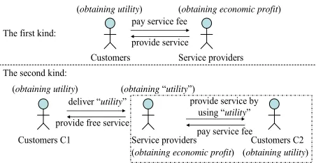
Moreover, according to different roles of v’s receiver and different kinds of service interaction, the meaning of Value Indicators is different. There are two types of role in service interaction: customers and service providers. There are two kinds of service interaction, as shown by
Figure 2. In the first hind, service providers provide ser-
vice for customers and charge customers for certain rea- sonable fees. In the second kind, service providers pro- vide free service for customers C1 and obtain some “util- ity”, and service providers provide service for customers C2 by utilizing the “utility” and charge customers C2 for certain reasonable fees. In the service interaction be- tween service providers and customers C1, service pro- vider only can obtain the indirect profit which is the economic profit may be transformed from the “utility” in the future during the service interaction between service providers and customers C2 occurring.
For the first kind of service interaction, the meaning of Value Indicators is given as follows. For customers, the value that he receives is customer value (represented as cv). The meaning of cv’ Value Indicators is given in Ta- ble 1. For service providers, the value that he receives is
provider value (represented as pv). The meaning of pv’ Value Indicators is also given in Table 1.
Satisfaction degree
v
B C E
Service elements
QoS=(q1,q2,…,qn)
fB
FunctionG
FunctionH
fC fE
[image:4.595.346.495.448.570.2]CON=(q1,q2,…,qm)
Figure 1. Thecomputation structure of service value.
Customers Service providers
pay service fee
provide service The first kind:
The second kind:
(obtaining utility) (obtaining economic profit)
Customers C1 Service providers
deliver “utility”
provide free service
(obtaining utility) (obtaining“utility”)
pay service fee provide service by
using “utility”
Customers C2 (obtaining utility) (obtaining economic profit)
[image:4.595.311.537.600.717.2]Table 1. The detailed information of six kinds of Value Indicators in the first kind of service interaction.
Value Indicators Nature Influencing Factor Initial Value of Value Indicators
cv_B Variable cv_CONB
cv_Bbest is the max amount of money that customers are willing to pay for the utility
that they perceived in the best service, which is proposed by customers.
cv_C Constant
cv_C is the amount of money that customers actually needed to pay for the obtained
service, and is the service price confirmed through the negotiation between customers and providers before the execution of service.
cv_E Variable cv_CONE
cv_Ebest is the max amount of money that customers can obtain when cv_CONE is best
fulfilled. cv_Ebest is proposed by providers.
pv_B Constant pv_B is confirmed through the negotiation before the execution of service. pv_B = cv_C
pv_C Variable pv_CONC pv_Cbest
is the max amount of money that providers pay for delivering the best service, which is proposed by providers.
pv_E Variable sat pv_Einteraction when sat is highest. best is the max amount of money that providers may obtain in the next service pv_Ebest is proposed by providers.
For the second kind of service interaction, the meaning of Value Indicators is given as follows. For customers, the meaning of cv_B and cv_C is the same as their meanings in the first kind of service interaction. But be- cause the service obtained by customers C1 is free, cv_C equals 0 and cv_E no longer exists.
For providers, the meaning of pv_B and pv_C is also the same as their meanings in the first kind of service interaction, especially pv_B equals 0. But the meaning of pv_E is different from its meaning in the first kind of service interaction. pv_E is the amount of money that service providers may obtain in the future by providing service for customer C2 by using the “utility” that is ob- tained from customer C1 in the current service interac- tion. It is affected by the value profit constraint pv_CONE proposed by providers. The quality parameters of pv_CONE are used to measure some specific characteris- tic of customers’ behavior. The initial value of pv_E is represented as pv_Ebest. pv_Ebest is the max amount of
money that providers may obtain by delivering the “util- ity” in the future when pv_CONE is best fulfilled. pv_Ebest
is proposed by providers.
2.3. Value Dependency Relationship
Service value does not exist independently. There could be value dependency relationship among multiple service values. Value dependency relationship is defined as the implementation degree of a service value is completely or partially dependent on one of the others, which is de- noted as
1, , ,2
i. Obviously, value de-g n
d v v v v
j
m
pendency relationship can affect the service value meas- urement. Dependency function g is used to measure the impact of
1 2 on i. As mentioned above, the value dependency relationship among multiple ser- vice values are caused by the uncertainty of relationships between various quality parameters of the corresponding service elements., , , n
v v v v
As shown in Figure 3, there are two service values vi
and vj, and vj is affected by vi. The value dependency relationship is denoted as d vi gv , where g is used to measure the impact of vi on vj. The impact is ac- tually caused by the uncertainty of relationships between the quality parameters of sej related to vj and the quality parameters of sei related to vi. A quality parameter of sei directly affects the corresponding one of sej, and can in- directly affect the corresponding quality parameters of vj’CON. And then it continues to indirectly affect vj’ value indicators, at last indirectly affect vj.
Value dependency relationship may be caused by one or more quality parameters of service elements. For one, its dependency function is denoted as g = P(Bh|Ak) (for
1,2, , ; 1,2, ,
k n h ) which represent the uncer- tainty of relationships between sej·qx and sei·qx (as men- tioned in Section 2.1). For more quality parameters, its dependency function is also represented as the set of conditional probability.
3. Measurement of Independent Service
Value
Independent service value refers to the service value that is not dependent on other service values. Its implementa- tion is not affected by the implementation of the others. It
Satisfaction degree
vi
B C E
CON=(q1,q2,…,qn)
Service element sei
QoS=(q1,q2,…,qm)
fB
FunctionG
FunctionH
fC fE
Satisfaction degree
vj
B C E
CON=(q1,q2,…,qn)
Service element sej
QoS=(q1,q2,…,qm)
fB
FunctionG
FunctionH
fC fE
g i j
d v v
g
[image:5.595.312.537.585.719.2]is measured only based on Qos of its corresponding ser- vice elements.
3.1. Independent Customer Value
In the first kind of service interaction, for cv, its cv_B is affected by cv_Bbest and cv_CONB, and its cv_E is af- fected by cv_Ebestand cv_CONE. Therefore, cv can be denoted as
bestbest
_ , _ _
_ , _ ,
B B
E
cv f cv B cv CON cv C
f cv E cv CON
E
where the function fB is:
_ _
where , _
S S H
best x x x x x
S H
x x B
cv B cv B w g q f q
q q cv CON
,(1)
In the formula (1), H x
q is the hard quality parameter, which means its expected constraint must be fulfilled. The function fx is used to measure whether
H x
q ’s ex- pected constraint can be fulfilled by the value of H
x
q . The proposition of H
x
q ’s expected constraint and the
H x
q ’s calculation is as follow. The quality parameter H
x
q ’s constraint is proposed by customers, and its constraint range is divided into the expected range and the unacceptable range. There are two kinds of quality parameters: the first one is that the bigger the quality parameter is, the higher the quality of the corresponding service is; and the second one is that the smaller the quality parameter is, the higher the qual- ity of the corresponding service is.
Taking H x
q that belongs to the first kind as an exam- ple, its expected range can be denoted as H
x e
q Q , and
H x
q ’s unacceptable range is denoted as qxH Qe, where Qeis the smallest one in all the acceptable values of qxH.
For H x
q , any values that do not belong to the expected range can not be acceptable.
The quality parameter H x
q is calculated based on the QoS of a service element (or a set of service elements). If
H x
q is related to a service element se, then
H
x x
q se q
cv . If qHx
, n
is related to a set of service ele- ments se se1, 2,
H se
, then
1 , 2 , ,
x x x x n
cv q G se q se q se qx , where according to different H
x
q and the different se- quence relationships between various service elements, the function Gxmay be one of the simple operations (e.g.
, , min, max etc.).
In order to express the meanings of H x
q in the for- mula (1), the range of
Hx x
f q is defined as {0, 1}, and the corresponding weight of
Hx x
f q is defined as 1. It is assumed that the range of H
x
q can be denoted as [min, max], then the function fxis:
For H
x
q belonging to the first kind, the function fx is
1 iff
,max
0 otherwise H
x e
H x x
q Q
f q
.
For H
x
q belonging to the second kind, the function fx
is
1 iff
min,
0 otherwise
H
x e
H x x
q Q
f q
.
If the value of H x
q belongs to the expected range,
H 1x x
f q , or else
H 0 x xf q . When
H 0x x f q , the weight of
Hx x
f q is 1, then cv_B = 0, which means that when the value of H
x
q is not belonging to the ex- pected range the value’s receiver will not be willing to pay any money.
In the formula (1), the part “ S
Sx x x
w g q
” is simi-lar to the formula to calculate the overall quality pro- posed by the reference [17]. The formula to calculate the overall quality is firstly to calculate the gaps between expectations of various quality parameters and their per- ceptions, and then, each gap multiplies with its weighting, and finally the result of the overall quality is obtained. The function
Sx x
g q is also related to the gaps be- tween expectations of various quality parameters S
x
q and their perceptions. But the objective of the function
S x xg q is not to simply calculate the gaps but to meas- ure the impact of the gaps on cv_Bbest. And then, each
impact degree multiplies with its weighting S x
w , and finally the result of cv_B is obtained. In this paper, the expectations of quality parameters are represented by the expected constraints that are proposed by value receivers, and the perceptions of quality parameters are represented by the values of quality parameters that are designed by service model designers.
In formulas (1), S x
q
S
is the soft quality parameter that means whether or to what degree its constraint is fulfilled is not strictly required. The function gx is used to measure whether or to what degree qx
S
’s expected constraint is fulfilled by the value of qx. wxS is the weight of
S x xg q , and S
0,1 xw . According to the importance
of
S x xg q to cv_B, wSx can be assigned by the experts
in correlative domains. Similar to H
x
q , qSx
S
is calculated based on the QoS of a service element (or a set of service elements), which is denoted as cv q x se qx or
1 , 2 , ,
S
x x x x
cv q G se q se q sen q
S
x
.
The quality parameter qx’s constraint is proposed by customers, and its constraint range is divided into the expected range, the acceptable range and the unaccept- able range. As the space is limited, taking S
x
q belonging to the first kind as an example, the proposition of S
x
q ’s constraintand some typical formulas of gx are given as follow.
For S x
of S x
q is denoted as qxS Qe, the unacceptable rangeof
S x
q is denoted as qxS Qa
S a x
Q q Q
S, and the acceptable range of qxS is denoted as e, where Qe is the smallest one in all the expected values, and Qathe smallest one in all the acceptable values.
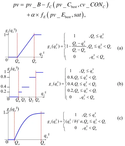
The range of gx qx is [0,1]. For
S x
q belonging to the first kind, some typical formulas and their images of the function gxis given as follow.
In Figure 4, the formula (a) is applicable to the case,
where the impact of S x
q ’s change on cv_B is linear. The formula (b) is applicable to the case, where the impact of
S x
q ’s change on cv_B is nonlinear and segmented. In the formula (c), 0 < a < 1, b > 0, it is applicable to the case, where the impact of S
x q _ _ E f pv f pv
’s change on cv_B is nonlinear and coincides with the law of marginal effect.
The approach for measuring cv_E is similar to cv_B measurement, and the only difference is that the con- straints of the quality parameters of cv_CONE and cv_Ebestare proposed by providers.
For the second kind of service interaction, as men- tioned above, for value cv, its value indicator cv_B is affected by cv_Bbestand cv_CONB, its value indicator cv_C is 0, and value indicator cv_E does not exist. Therefore, cv can is denoted as cv = fB(cv_Bbest, cv_CONB), where the function fB is the same as the function fB which is used in the first kind of service interaction.
3.2. Independent Provider Value
In the first kind of service interaction, for pv, its pv_C is affected by pv_Cbest and pv_CONC, and its pv_E is af- fected by pv_Ebestand Sat. Therefore, pv can be denoted
as
best, _
_ , ,
C
pv pv C cv CON
sat
C best E B 0 Qa Qe
1gx(qxS)
qxS
0 0.8
Qe QaQ1 Q2
1
0.4 0.2
q gx(qxS)
xS 1 , 1 , 0 , S e x S
S e x S
a x e e a S x a Q q Q q ( ) x x
g q Q q Q
Q Q q Q 2 1 2 1 1 , 0.8, 0.4, 0.2, 0 , S e x S x e S x S a x S x a Q q
Q q Q
Q q Q
Q q Q
q Q 1 , ( / ) , 0 , S e x
S S S
x a x e S x a Q q
( )S x x g q ( ) x x
g q q b a Q q Q
q Q (a) (b) 0 1 Qe Qa qx
gx(qxS)
[image:7.595.71.280.476.721.2](c) S
Figure 4. Some typical formulas of the function gx.
where the function fC is:
best
_ _ ,
where _
x x x
x C
pv C pv C w h q
q pv CON
(2)
In formula (2), the function hx is used to measure the degreethat the constraint of the quality parameter qx is fulfilled by the value of qx·wxis the weight of hx(qx), and wx (0,1). According to the importance of hx(qx)to pv_C, wx can be assigned by the correlative domain experts. The quality parameter qx is calculated based on the QoS of a service element (or a set of service elements), which is denoted as pv q x se qx or
1 , 2 , ,
x x x x n
pv q G se q se q se qx .
The quality parameter qx’s constraint is proposed by providers, and its constraint range is divided into the biggest cost range, the variable cost range and the small- est cost range. As the space is limited, taking qx belong- ing to the first kind as an example, the proposition of qx’s constraintand some typical formulas of the function hx are given as follow.
For qx belonging to the first kind, the biggest cost rangeof qx is denoted as qxQend, the smallest cost range
of qx is denoted as qx< Qstart, and the variable cost range
of qx is denoted as Qstart qx < Qend, where Qstart is the
smallest value of qx which can cause the change of hx(qx) that represents the impact of qx’s change on pv_C, and Qend is the biggest value of qx which can cause the change of hx(qx). Qend is actually the smallest value of qx which service providers can provide by paying the biggest cost.
In actual services, the cost that providers pay is impos- sible to become infinitely smaller along with that the quality of the service that providers deliver to customers becomes infinitely lower. Therefore, the range of hx(qx) is defined as [,1]. If all the quality parameters of pv_CONC belong to the smallest cost range, pv_Cmin =
pv_Cbest . The cost pv_Cmin is the smallest value of
pv_C. Some typical formulas and their images of the function hx are given as follow.
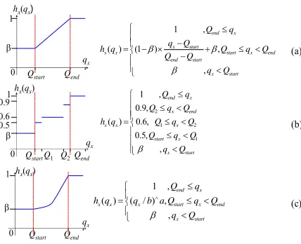
In Figure 5, the formula (a) is applicable to the case,
where the impact of qx’s change on pv_C is linear. In the variable cost range, the change of qx makes the hx(qx) change, and the rate of change of hx(qx) is constant. The formula (b) is applicable to the case, where the impact of qx’s change on pv_C is nonlinear and segmented. In a subrange of the variable cost range, sometimes the change of qx can not make the hx(qx) change, and some- times the tiny change of qx can cause the step change of hx(qx).
(a)
(b)
(c) 0
1
Qstart Qend
qx
hx(qx)
0 0.9
QstartQ1 Q2Qend
1
0.6
qx
hx(qx)
0.5
0 Qstart Qend
1
qx
hx(qx)
1 ,
( ) (1 ) ,
,
end x x start
x x start x end
end start x start Q q q Q
h q Q q Q
Q Q q Q
2
1 2
1
1 ,
0.9, ( ) 0.6, 0.5,
,
end x x end
x x x
start x x start Q q Q q Q
h q Q q Q
Q q Q q Q
1 ,
( ) ( / ) ,
,
end x
x x x start x end
x start
Q q
h q q b a Q q Q
q Q
[image:8.595.307.537.83.270.2]
Figure 5. Some typical formulas of the function hx.
(from Qstart to Qend), the rate of change of hx(qx) is lower. And the rate of change becomes higher gradually with the increase of qx. Sometimes a combination of many kinds of formulas may also be selected for applying to some complicated service situation.
The function fEis used to measure the impact of sat on pv_E, which is denoted as fE(pv_Ebest, sat) = pv_Ebest
sat, where pv_Ebest is the max amount of money that pro-
viders may obtain in the next service interaction, and pv_Ebest may be assigned to a value by some forecasting
method [18]; sat is enumerated type, and its range is the fuzzy set {very satisfied, satisfied, poorly satisfied, un- satisfied}. In order to support the measurement of pv_E, the fuzzy set of sat may be quantified using the set {1, 0.8, 0.4, 0}, where very satisfied corresponds to 1, satis- fied corresponds to 0.8, and so on. As mentioned in the above Figure 2, sat is dependent on cv, which is denoted as sat = H(cv). The function H is used to measure the impact of the implementation degree of cv on sat. The formulas mentioned in Figure 6 may be adapted to in-
stantiate the function H when Qe is defined as the small- est cv in all the cv that customers expect to obtain and Qa is defined as the smallest cv in all the cv that customers can accept.
For the second kind of service interaction, as men- tioned above, for the value pv, its value indicator pv_B is 0, its value indicator pv_C is affected by pv_Cbestand
pv_CONC, and its value indicator pv_E is affected by pv_Ebestand pv_CONE. Therefore, pv can be denoted as
best
best
0 _ , _
_ , _
C C
E E
pv f pv C pv CON
f pv E pv CON
where the function fC is the same as the function fC which is used in the first kind of service interaction.
The function fE is different from the function fE which is used in the first kind of service interaction. The func- tion fE is similar to the formula (1) in the Section 3.1
T1 T2
T3 T4 T5 T6
E
E S
S CN
FR
S
SC T7 E
CN: consigners FR: forwarders SC: ship company
Request information
Cabin Information
Cabin booking Information Cabin information
Figure 6. Service process model for the first solution.
which is used to calculate the function fB of cv in the first kind of service interaction. The difference is that the constraints of the quality parameters of pv_CONE and pv_Ebestare proposed by providers. The quality parame-
ters of pv_CONE are used to measure some specific characteristic of customers’ behavior. In order to support the measurement of pv_E, some new quality parameters are need to be added into the Table 2 in the Section 2.2,
for example, a quality parameter that is used to measure whether customers register to be free member, a quality parameter that is used to measure whether customers responded to the questionnaires after obtaining service, and so on.
4. Measurement of Non-Independent Service
Value
Non-independent service value refers to the service value that is dependent on other service values. Its implemen- tation of non-independent service value is completely or partially affected by one of the others. The dependency function g should be used to support the non-independent value measurement. For the first kind of service interac- tion or the second one, whether a non-independent value is cv or pv, its measurement process is similar to the one of an independent one. There is only one difference: the quality parameters of CON are calculated based not only on the QoS of the corresponding service elements but also on the corresponding dependency function g.
The dependency relationship
1, , ,2
g
n j
d v v v v
is caused by the uncertainty of relationship between the quality parameters of their corresponding service ele- ments (sej is related to vj, and se se1, 2, , sen is related to 1 2 respectively). Therefore, if a quality pa-
rameter qx of vj. CON is affected by the uncertainty, the , , , n
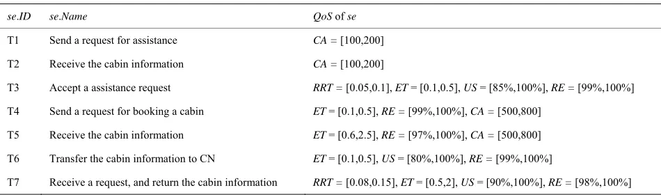
[image:8.595.66.280.84.258.2]Table 2. The detailed information of service tasks.
se.ID se.Name QoS of se
T1 Send a request for assistance CA = [100,200]
T2 Receive the cabin information CA = [100,200]
T3 Accept a assistance request RRT = [0.05,0.1], ET = [0.1,0.5], US = [85%,100%], RE = [99%,100%]
T4 Send a request for booking a cabin ET = [0.1,0.5], RE = [99%,100%], CA = [500,800]
T5 Receive the cabin information ET = [0.6,2.5], RE = [97%,100%], CA = [500,800]
T6 Transfer the cabin information to CN ET = [0.1,0.5], US = [80%,100%], RE = [99%,100%]
T7 Receive a request, and return the cabin information RRT = [0.08,0.15], ET = [0.5,2], US = [90%,100%], RE = [98%,100%]
RRT: Request response time; ET: Execution time; US: Usability; RE: Reliability; CA: Consumption amount.
transformed from the probability set “P B
bh
ph,1,2, , h
measurement of qx refers to not only the quality parame- ter sejqx but also thequality parameter set
1 x, 2 x, , n
m
”, therefore, pv2qx can be calculated by using the multiply operation of matrix. The data of the matrix (P(Bh|Ak))nm should be provided by service model designers, and the data of the matrix M(A) may be ob- tained by analyzing all relevant historical data.
x
se q se q se q .
And because the dependency function g is used to meas- ure the uncer tainty of relationship between sejqx and
se q se1 x, 2qx, , senqx
, the dependency function gshould be taken into consideration while calculating the quality parameter qx of vj·CON. Because of the effect of the dependency function g, the value of the quality pa- rameter qx may not be a single range, but a set of range in which each range is with a probability.
To bring pv2qx to the formula (2), and
2
x x
h pv q may be a set of values in which each value is with a probability, at last it may result in that pv2 may
also be a probability distribution.
If there are two quality parameters qx and qy which are related to the uncertainty of relationship, then the de- pendency function can be denoted as g = {P(Bh|Ak) (for
1,2, , ; 1,2, ,
k n h
Taking the service value pv as an example, how to cal- culate the quality parameters of CON of a non-inde- pendent value is given as follow.
m
), P(Dh|Ck) (for k1,2, , n; 1,2, ,
h m)}. The discrete random variable C repre- sents the value of quality parameter se1·qy. The discrete random variable D is the value of quality parameter It is assumed that there is a value dependency rela-
tionship 1 2, which is caused by the un- certainty of relationship between the quality parameters of se2 and se1 (se1, se2 is related to pv1 and pv2 respec-
tively).
g
dpv pv
2 y
se q .
Therefore, pv2·qx is the probability set P B
bh
ph,1,2, , h
If only one quality parameter qx of pv2·CON is related
to the uncertainty of relationship, the dependency func- tion can be denoted as g = P(Bh|Ak) (for ;
).
1,2, ,
k n
1,2, ,
h m
As mentioned above, pv2qxse2qx, and se2qx depends on se q1 x
k pk
and g. The probability set
“ , ” may be transformed
into the matrix
P Aa k 1,2, , n
P Aa1 ,P Aa2 ,,
n
m
P Aa . The set of conditional probability P(Bh|Ak) (for
) may also be transformed 1,2, , ;
k n h1,2,,
m
. and pv2qy is the probability set
P Ddh p dh, 1,2, , m. To bring pv2qx and
2 y
pv q to the formula (2), x
2 x
and hy(pv2·qy) can be obtained respectively. If the amount of members of the probability set related toh pv q
2
x x is K and
the one related to
h pv q
2
y y
h pv q is L, then at last, by car- rying on synthetical calculation, the amount of members of the probability set related to pv2 may be K L.
into the matrix
h k
n m P B A .
T
1 2
1 2
, , ,
, , ,
m
n
h k n m
P B b P B b P B b
P A a P A a P A a
P B A
In the above measurement process, the result of the function h and the result of the value indicators pv_C are always a set of probability. For these probability sets, their corresponding event may be the same, which results in that the amount of members of the probability set re- lated to output is less than the one related to input. In the most extreme case imaginable, pv2 is a probability of an
event, and the probability is 100%.
and
P B
b1
, andP B
b2
, , P B
bm
T can be5. Case Study
As mentioned in Section 1, there are two service solu- tions for cabin booking service. In the first service solu- tion, the consigners send a request to the forwarders, asking the forwarders to help him to book a cabin. The corresponding pre-designed service process model is shown in Figure 6. The detailed information of service
tasks in this model is listed in Table 2.
In this service process model, the quality parameter T7.ET, T5.ET and their relationship are uncertain. The uncertainty of T7.ET is denoted as P{A = ak} = pk, k = 1, 2. A1 is “A = [0.5,1]”, and A2 is “A = [1,2]”. The uncer-
tainty of T5.ET is denoted as P{B = bh} = ph, h = 1, 2, 3. B1 is “B = [0.6,1]”, B2 is “B = [1,2]”, and B3 is “B =
[2,2.5]”. And the set of conditional probability P(Bh|Ak) (for k = 1, 2; h = 1, 2, 3) = {{P(B1|A1) = 5%, P(B2|A1) =
80%, P(B3|A1) = 15%}, {P(B1|A2) = 0%, P(B2|A2) = 70%,
P(B3|A2) = 30%}} can be used to describe the uncertainty
of the relationship between T7.ET and T5.ET. The ser- vice process model and its relevant data are supposed to be collected and provided by model designers.
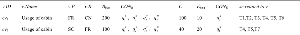
In the first solution, there are two service values cv1
and cv2. Their detailed information is given in Table 3.
In this example, the unit of all the value indicators is Yuan.
2= 2_ 2_ + 2_
cv cv B cv C cv E, where cv2_B and cv2_E
is calculated as follow:
3
2 2 best 4 4
1
_ _ H S
i i i i
cv B cv B f q w g q
S ,whereqiS, q4H cv2_CONB, and they are calculated as follow:
1S
q = T7.RRT =[0.08,0.15];
q2S = T7.
ET =[0.5,2];
3S
q = T7.US= [90%,100%];
4H
q = T7.RE =[98%,100%].
2_Ecv2_Ebestg5 qS
5 2_
S
5
cv , where
E
q cv CON , and q5S = T4.CA+T5.CA = [1000,
1600].
The constraints for q1S , q2S , q3S , q4H have been
proposed by the forwarders. The constraints for q5S have
been proposed by the ship company. And then the formulas of the functions 1
1S
g q , 2
2S
g q , 3
3S
g q ,
4 4
H
f q and 5
5S
g q are shown in Figure 7.
In the formula to caulcualte cv2_B, the weights of the
functions 1
1S
g q , g2
q2S , g3
q3S are assigned to0.4, 0.4, 0.2 respectively. Therefore, the results can be obtained: 1
1 0.8S
g q , g2
q2S 0.8 , g3
q3S 1 ,
4 4H
f q 1, g5
q5S 0.4, and thencv2 = 84 – 40 + 8 =
52 (Yuan).
1 1_ 1_ 1
cv cv Bcv C cv _E
S
q
. cv1 is dependent
on cv2, and the dependency function is P(Bh|Ak) (for k = 1, 2; h = 1, 2, 3). The calculationof cv1 is similar to the one
of cv2, only one difference is that the quality parameter
1 2
cv is calculated based on not only the quality pa-rameters T3.ET, T4.ET, T5.ET, T6.ET (related to cv1) but
also the quality parameter T7.ET (related to cv2).
3
1 1 best 4 4
1
_ _ H S
i i i i
cv B cv B f q w g q
SB
,
where , and they are calculated as
follow: 4 1
, _
S H i
q q cv CON
1S
q = T3.RRT = [0.05,0.1];
2S
q = T3.ET + T4.ET + T5.ET + T6.ET = [0.3,1.5] + T5.ET;
3S
q = min(T3.US, T6.US) = [80%,100%];
4H
q = T3.RE T4.RE T5.RE T6.RE = [94%, 100%].
The constraints for 1 2
S
cv q have been proposed by the consigners. And then in the formula to calculate cv1_B, the formulas of the function g2
q2S is
2 2
2 2 2
2 2
0, 6
0.2, 4 6
0.4, 3 4
0.8, 2 3
1, 2
S
S
S S
S
S q
q
g q q
q
q
.
The formulas of the other functions in the formula to caulcualte cv1_B are the same as the corresponding ones
in the formula to caulcualte cv2_B.
By analyzing all relevant historical data, P{A = [0.5,1]} = 80% and P{A = [1,2]} = 20% can be obtained. And then T5.ET can be calcualted by utilizing the multiply operation of matrix “(P{A = [0.5,1]}, P{A = [1,2]}) (P(Bh|Ak))23”. The results of T5.ET can be obtained: P(B
= [0.6,1]) = 4%, P(B = [1,2]) = 78% and P(B = [2,2.5]) = 18%. Therefore, the results of cv q1 2S and 2
1 2
[image:10.595.59.537.664.721.2]S g cv q can be given as follow:
Table 3. The detailed information of two values belonging to cv.
v.ID v.Name v.P v.R Bbest CONB C Ebest CONE se related to v
cv1 Usage of cabin FR CN 200 1
S
q , 2, ,
S
q 3
S
q 4
H
q 100 10 5
S
q T1,T2, T3, T4, T5, T6
cv2 Usage of cabin SC FR 100 1
S
q , 2, ,
S
q 3
S
q 4
H
q 40 20 5
S
q T4, T5,T7
1
S
q 2
S
q 3
S
q
: Request response time; : Execution time; : Usability; 4 : Reliability; : Consumption amount.
H
q 5
S
1 1
1 1 1
1 1
0, 0.25 0.2,0.2 0.25 1) ( ) 0.4,0.15 0.2 0.8,0.1 0.15
1, 0.1 S S S S S S q q
g q q
q q 2 2
2 2 2
2 2
0, 6 0.2, 4 6 2) ( ) 0.4, 2 4 0.8,0.5 2 1, 0.5 S S S S S S q q
g q q
q q 3 3
3 3 3
3 3
1, 0.9 0.8, 0.6 0.9 3) ( ) 0.4, 0.5 0.6 0.2, 0.3 0.5
0, 0.3 S S S S S S q q
g q q
q q 4 4 4 4 1,0.9 4) ( )
0, 0.9 H H H q f q q 5 5
5 5 5
5 5
1, 2000 0.8, 1500 2000 5) ( ) 0.4,1000 1500 0.2, 500 1000 0, 500 S S S S S S q q
g q q
[image:11.595.103.529.79.501.2]q q
Figure 7. The formulas of the functions
Sg q1 1 ,
Sg2 q2 ,
Sg3 q3 ,
Hf4 q4 and
Sg5 q5 . B1 is the event “B = [0.6,1]”, if B1 occurred,
1 2 0.9, 2.5
S
cv q , 2
1 2S
0.8; g cv q B2 is the event “B = [1,2]”, if B2 occurred,
1 2 1.3,3.5
S
cv q , g2
cv q1 2S
0.4; B3 is the event “B = [2,2.5]”, if B3 occurred,
1 2 2.3, 4
S
cv q , g2
cv q1 2S
0.4.And then by utilizing the other corresponding formulas
of function, , and
can be obtained. 1
1 1
1 Sg cv q
1 3
1 3
0.8S g cv q
S
4 1 4
H f cv q
1_ 1_ best 5
cv Ecv E g q5 ,
where q5Scv1_CONE, and = T1.CA + T2.CA =
[200,400]. 5
S
q
The constraints for 1 5 have been proposed by
the forwarders. And then in the formula to calculate cv1_E, the formulas of the function
S
cv q
5 5 S g q S is
5 5 5 5 5 5 5 1, 5000.8, 200 500
0.4, 100 200
0.2, 50 100
0, 50. S S S S S q q g q q q q
So, can be obtained. At last, the
measurement result of cv1 is: P{cv1 = 84} = 4%, P{cv1 =
52} = 96%.
5 1 5 0.8
S g cv q
In the first solution, there are two service values pv1
and pv2. The detailed information is given in Table 4.
2 2_ 2_ 2
pv pv Bpv C pv _E , where pv2_C
and pv2_E is calculated as follow:
4
2 2 best
1 2
_ _
where _
i i i i
i C
pv C pv C w h q
q pv CON
, and they are calculated as follow:
q1 = T7.ET = [0.08,0.15]; q2 = T7.ET = [0.5,2]; q3 = T7.US = [90%,100%]; q4 = T7.RE =[98%,100%].
pv2_E = pv2_Ebestsat.
In the above two formulas, the formulas of the func- tions h1(q1), h2(q2), h3(q3), h4(q4) are:
1
1
1 1 1
1
1
0.3, 0.25
0.5, 0.2 0.25
0.6, 0.15 0.2
0.9, 0.05 0.15
1, 0.05
q
q
h q q
q q
2 22 2 2
2
2
0.3, 6
0.5, 4 6
0.6, 2 4
0.9, 0.5 2
1, 0.5
q
q
h q q
q q
3 33 3 3
3
3
1, 0.8
0.9, 0.6 0.8
0.6, 0.4 0.6
0.5, 0.2 0.4
0.3, 0.2
q
q
h q q
q q
4 44 4 4
4
4
1, 0.9
0.9, 0.8 0.9
0.6, 0.7 0.8
0.5, 0.6 0.7
0.3, 0.6
q
q
h q q
q q .
And then the weights of the functions h1(q1), h2(q2),
h3(q3) and h4(q4) are assigned to 0.3, 0.3, 0.2, 0.2 respec-
tively. Therefore, pv2 = 40 – 9.7 + 16 = 46.3 (Yuan). Re-
ferring to the measurement process of pv2 and cv1, the
measurement result of pv1 can be obtained: P{pv1 = 65.7}
= 82%, P{pv1 = 71.2} = 18%.
In the second solution, the consigners directly send a request to the ship company for booking a cabin. The detailed information of the corresponding pre-designed service tasks is listed in Table 5. Simultaneously, there
are two service values cv1 and pv1 in this solution, as
shown in Tables 6 and 7. The measurement process of
cv1 and pv1 is similar in the first solution, and result is
given in Table 8.
The comparison results between the first and the second service solution is shown in Table 8. As the table
[image:11.595.344.494.144.503.2]