Aperiodic Checkpoint Placement Algorithms—Survey and Comparison

http://dx.doi.org/10.4236/jsea.2013.64A006 Published Online April 2013 (http://www.scirp.org/journal/jsea)

Aperiodic Checkpoint Placement Algorithms—Survey and

Comparison

*

Shunsuke Hiroyama, Tadashi Dohi, Hiroyuki Okamura

Department of Information Engineering, Hiroshima University, Hiroshima, Japan. Email: [email protected], [email protected]

Received January 23rd, 2013; revised February 24th, 2013; accepted March 4th, 2013

Copyright © 2013 Shunsuke Hiroyama et al. This is an open access article distributed under the Creative Commons Attribution Li-cense, which permits unrestricted use, distribution, and reproduction in any medium, provided the original work is properly cited.

ABSTRACT

In this article we summarize some aperiodic checkpoint placement algorithms for a software system over infinite and finite operation time horizons, and compare them in terms of computational accuracy. The underlying problem is for-mulated as the maximization of steady-state system availability and is to determine the optimal aperiodic checkpoint sequence. We present two exact computation algorithms in both forward and backward manners and two approximate ones; constant hazard approximation and fluid approximation, toward this end. In numerical examples with Weibull system failure time distribution, it is shown that the combined algorithm with the fluid approximation can calculate ef-fectively the exact solutions on the optimal aperiodic checkpoint sequence.

Keywords: Checkpoint Placement; Aperiodic Policy; Availability Models; Computation Algorithms; Comparison

1. Introduction

It is well known that the system failure in large-scale computer systems can lead to a huge economic or critical social loss. Checkpointing and rollback recovery is a commonly used technique for improving the reliabil-ity/availability of fault-tolerant computing systems, and is regarded as a low-cost software dependability tech-nique from the standpoint of environment diversity. Es-pecially, when file systems to write and/or read data are designed, checkpoint (CP) generations back up periodi-cally/aperiodically the significant data on a primary me-dium to safe secondary media, and play a significant role to limit the amount of data processing for recovery ac-tions after system failures occur. If CPs are frequently taken, a larger overhead will be incurred. Conversely, if only a few CPs are taken, a larger overhead after a sys-tem failure will be required in rollback recovery actions. Hence, it is important to determine the optimal CP se-quence taking account of the trade-off between two kinds

of overhead factor above. In many cases, the system fail- ure phenomenon is described with a probability distribu-tion called the system-failure time distribution, and the optimal CP sequence is determined based on any sto-chastic model. For the excellent survey on this topic, see [2,3].

First Young [4] obtains the optimal CP interval ap-proximately for a computation restart after system fail-ures. Baccelli [5], Chandy et al. [6,7], Dohi et al. [8-10], Gelenbe and Derochette [11], Gelenbe [12], Gelenbe and Hernandez [13], Goes and Sumita [14], Goes [15], Grassi

et al. [16], Kobayashi and Dohi [17], Kulkarni et al. [18], Nicola and van Spanje [19], Sumita et al. [20], among others, propose performance evaluation models for data-base recovery, and calculate the optimal CP intervals which maximize the system availability or minimize the mean overhead during the normal operation. L’Ecuyer and Malenfant [21] formulate a dynamic CP placement problem by a Markov decision process. Ziv and Bruck [22] analyze an online algorithm for a probabilistic CP placement. Vaidya [23] examines an impact of check-point latency on overhead ratio for a simple CP model. Okamura et al. [24] reformulate the Vaidya model [23] with a semi-Markov decision process and further develop a reinforcement adaptive learning algorithm for CP placement. For several CP models in the literature, the periodic CP intervals are implicitly assumed. This is

*_{This is an extended version of the conference paper [1] presented at}

The 2nd International Conference on Advanced Computer Science and Information Technology (AST 2010), Miyazaki, Japan, June 23-25, 2010.

because the periodic CP intervals maximize the steady- state system availability, and in many cases, are better than the randomized CP ones which are given by inde- pendent and identically distributed random variables. However, it is worth noting that the periodic CP strate-gies can not be always validated in some cases and less performe than the aperiodic CP placement. In general, it is known that the way to place the optimal CP sequence strongly depends on both kind of objective functions (system availability, mean overhead, etc.) and kind of system-failure time distribution. Since the aperiodic CP involves the periodic CP as a special case, it is meaning-ful to consider the aperiodic CP placement algorithm for file systems.

When the system-failure time obeys a non-exponen- tial distribution, it is easily shown that the aperiodic CP placement is not worse than the periodic CP one. Toueg and Babao lu [25] develop a dynamic programming (DP) algorithm which minimizes expected execution time of tasks placing CPs between two consecutive tasks under very general assumptions. Kaio and Osaki [26] consider an approximate aperiodic CP placement algo-rithm under the asssumption that the conditional sys-tem-failure probability is constant during the successive CPs. Fukumoto et al. [27,28] and Ling et al. [29] propose fluid approximation methods based on a variational cal-culus approach to derive the cost-optimal aperiodic CP sequence. Ozaki et al. [30,31] give an exact aperiodic CP placement algorithm and further develop an estimation scheme under the incomplete knowledge on system- failure time distribution. In a fashion similar to the above approach, Dohi et al. [32] formulate another aperiodic CP placement problem with equality constraints. Iwa-moto et al. [33], Okamura et al. [34,35], and Okamura and Dohi [36] propose different DP-based algorithms from Toueg and Babao lu [25] under the availability criterion, by taking account of another dependability technique, called the software rejuvenation in the pre-sense of software aging, where the system failure caused by the aging is not exponentially distributed. Recently, Ozaki et al. [37] propose a fixed-point type algorithm for an aperiodic CP placement with an infinite opera-tion-time horizon. In this way, considerable attentions have been paid for aperiodic CP placement problems in past.

g

g

Nevertheless, it can be pointed out that no effective aperiodic CP placement algorithm has been known yet when the number of CPs is very large. The constant haz-ard approximation [26] and fluid approximation [27-29] may poorly work in such a case. The search-based itera-tion algorithm in [30,31] and the DP-based algorithm in [33-36], which are regarded as exact computation algo-rithms, also require the very careful adjustment to deter-mine the number of CPs if the operation time for a file

system is finite. As the operation time becomes longer, in general, the number of CPs is sensitive to not only the determination of the aperiodic CP sequence but also the resulting dependability measures. In this article we sum- marize some aperiodic CP placement algorithms for a software system over infinite and finite operationtime horizons, and compare them in terms of computational accuracy. It is proposed to combine the fluid approxima- tion with an exact computation algorithm in determining the initial value of the number of CPs. The idea is quite simple, but we show that the combined algorithm with the fluid approximation can calculate effectively the ex- act solutions on the optimal aperiodic CP sequence.

2. Formulation of Optimal CP Placement

First, consider a centralized file system with sequential checkpoint (CP) over an infinite time horizon. The system operation starts at time , and the CP is sequentially placed at time 1 2 to back up the data processed in the file system. At each CP,

0 t



t t, ,,t_k,





1, 2,



k

t k  , all the file data on the main memory is saved to a safe secondary medium, where the fixed cost (time overhead) c0

 

0 is needed per each CP place- ment. It is assumed that the system operation stops during the checkpointing, so during the period 0 the file system does not deteriorate. System failure may occur according to an absolutely continuous and non-de- creasing probability distribution function

c

 

F t having density function f t

 

and finite mean . Upon a system failure, a rollback recovery takes place imme- diately where the file data saved at the last CP creation is used. Next, a CP restart is performed and the file data is recovered to the state just before the system failure occurs. The time length required for the CP restart is given by the function



0





 



 





L , which depends on the system failure time, and is assumed to be differentiable and increasing. We call the function the recovery

function in this article. After the completion of CP restart, an additional CP must be created to save the current state and the system operation restarts with the same condition as the initial point of time t . The similar cycle repeats again and again over an infinite time horizon.

L

0

The problem is to determine the optimal CP sequence



t t t1, , ,2 3



 

t maximizing the steady-state system

availability:

 

 

 

0 ₀

 

 

d

d

F t t AV

V t

V t F t t

 



  

 

 

 

 





t (1)

where

 

1





F   F 

and

 

1









 

0 0

1 d

k k t

k t

k

V    c k L t t



 





_    _

denotes the expected operaing cost with t00. It is evident that the underlying problem is reduced to a simple minimization problem t_   . In this pro-

blem, the expected recovery cost is usually given by the affine form



min V t





k



0



k



0



k, 0,1, 2,



L t t a t t b t t k   for the system failure time , where and

are given constants. Instead, by replacing the above CP cost and recovery cost by and

t a₀



0







 

0 0

b 

[image:3.595.363.539.327.464.2]

L t , this is equivallent to the clas- 0 sical inspection problem by Barlow and Proschan [38]. Figure 1 illustrates the configuration of the underly- ing CP placement with a finite operation-time horizon

.

c k



k1 t



a t0



k1t

 

0 T 

From the analogy to the inspection problem, it can be easily shown that the optimal CP sequence



t t t1, , ,2 3

   

  

t

 

maximizing the steady-state system availability is a non-increasing sequence under the assumption that the system failure time distribution

F t

t    t t t t

is PF2 (Polya Frequency Function of Order 2) [38], if there exists the optimal CP sequence satisfying

1 2 1 3 2 . Then, it must satisfy the fol- lowing first order condition of optimality:

t_



   

 

1 ₀ 1 0 . k k k k k

F t F t _c

t t a f t       _ 

   (3)

From the condition of optimality, an algorithm to de-

rive the optimal CP sequence which

minimezes or equivalentlly maximizes can be derived as follows.



t t t1, , ,2 3



   

  

t

 

V_ t_

 

AV_ t_

Forward CP Placement Algorithm for an Infinite Operation-Time Horizon: [30,31,37].

Step 1: Set t1 satisfying

 

 

.

1

0 0 ₀ d 0 1

t

c a

_

t F t b F t

Step 2: Compute t



t t t2, , ,3 4  using Equation (3).

1, 2, 3, k 



Step 3: For -th CP , if

, then decrease and Go to Step 2.

k k t   k





1 t



k1, 2, 3,



1 1

Step 4: For -th CP , if

k k k

t   t t

 tk₁ tk 0

t  t t

, then increase 1 and Go to Step 2.

Step 5: For the resulting CP sequence 1 2 k, if

k

t , then Stop the

procedure, where

t









 

1

0 1 d

k t

k

c k L t t F t



     

 





 

0



1 0

k k

t  t

is sufficiently small tolerance

value and .

Figure 1. Configuration of the aperiodic CP placement with a finite operation-time horizon T.

In the above algorithm, arbitrary increasing and de- creasing operations in Steps 3 and 4 can be taken to speed up the computation. The simplest method would be the bisection serach method. As the simplest case, if the system failure time is given by the exponential distri- bution with mean , it is well known that the optimal CP sequence is periodic, i.e.,

1 2 1 3 2

t     t t t t .

Since the processing time for a given transaction is in general bounded, the CP placement for an infinite-time horizon may be questionable in many practical applica- tions. As a natural extension of the infinite-time horizon problem, it would be interesting to consider the finite operation-time horizon problem, because is a special case. Suppose that the time horizon of operation for the file system is finite, say, , which can be regarded as a fixed transaction processing time. For a finite sequence

T 



0 T 





1, ,2 ,



N  t t  tN

t , the expected ope-

rating cost is given by

 













  



  

 





 







 

1 1 1 0 0 0 0 1 0 0 0 0 0 1 d 1 d 1 d 1 , k k N k k T N t N k k t t N k k k t N k k t V

c k L t t F t

c N F t

c k F t F t

a t t b F t c N F t

         _    _     _  _  _   _  

 





 

t (4)

where Nmin



k t: k1T



T

. Also we suppose that the file system restarts with a fixed CP overhead c0 just after the time , if the system failure does not occur. Since the steady-state system availability is given by

 

 

 

 

0 0 d , d T

T N T

T N

F t t AV

V F t

 





t t t (5)

the underlying maximization problem reduces to

 

min_t V t

t 

N T N . It should be noted that the recovery cost

does not occur at . To simplify the notation, we define N 1

t T

T

 in this article. When the recocery cost function is the affine form i.e., L t

 

a t b0  0 , dif- ferentiating Equation (4) with respect to t k_k 1, 2,



 ,N



and setting it equal to 0 yield Equation (3) again for





1 0 1, 2, 3, ,

k k

t t _  k  N and a given N.

Since the finite operation-time horizon problem invo- lves the constraint on the number of CPs, it is impo- ssible to apply directly the forward CP placement algo- rithm for an infinite operation-time horizon problem. However, by adjusting the value of , we can develop the similar algorithm to compute the optimal CP sequ-

N

[image:3.595.76.268.635.708.2]

ence. The basic idea is to utilize the non-increasing pro- perty of CP sequence under the PF2 assumption for an arbitrary number . Based on the result for an infinite time horizon [30,31,37], we modify the forward CP place- ment algorithm as follows.

N

T

Forward CP Placement Algorithm for a Finite Opera- tion-Time Horizon: [30,31].

Step 1: Set the lower and upper bounds of by and , respectively.

1 t : 0

l

z  z_u

Step 2: 1:



l



2

0, k

t z zu N .

Step 3: For , compute the CP sequence by

1,, 1

2, ,2 , N, N

t t  t t 

  

  

1 0

1 1

0 :

k k k k k

c

t F F t t t f t

a      _     .   

Step 4: For 1, 2 ,

k k

t t

1

k k

t  t

u

:

l

z , ,

k  N

t

  

Step 4.1: If , then and Go to Step 2.

1 k tk 1

  zut1

Step 4.2: If , then and Go to Step 2.

0

  zlt1

Step 5: For an arbitrary tolerance level , if , then and Go to Step 2.





1 1

Step 6: For an arbitrary tolerance level , if , then and Go to Step 2. N

t    T  z :t

1

Step 7: End. N

t   T  t1

For all possible combinations of , we calculate all expected operating costs using the above algorithm, and determine both the optimal number of CPs,

N

N

and its associated CP sequence N



1, ,2 , N



. It should be noted that the above two algorithms can be validated only when the system failure time distribution is PF2 and the resulting CP sequence is non-increasing, i.e.,

1

k k . The most significant point is that these algo- rithms are very fast to derive the optimal CP sequence, but strongly depend on the initial value 1. In the worst case, it is evident that these algorithms are sometime unstable and that the resulting CP sequence may not converge to the optimal solution. To overcome this point, the careful selection of the initial value 1 is essentially needed, so we improve it by the following algorithm.

t _ t t

t

t t_

t t

Improved Forward CP Placement Algorithm for a Finite Operation-Time Horizon:

Step 1: Set 1 , , and the upper bound of serach range .

0



0



1  1 1, k t j 1 N N



1 t   5 1.0 10  



N



Max

Step 2: Set and V0 . Step 2.1: t : t t.

Step 2.2: For , compute satisfying

,

 t_k1 1, 2,



i ,N

  

  

1 0

1 1

0 :

k k k k k

c

t F F t t t f t

a      _     .  

Step 2.3: Compute the corresponding expected operating cost and set it as Vj based on tk1 1, 2,



k ,N .

Step 2.4: If Vj1Vj, then VN Vj1 and tN tj1, and Go to Step 3, otherwise and Go to Step 2.1, where .

1 j j

4

1 10

 

j

Step 3: If t_kT k



1,2,,N



and NNMax, then 1

N N and Go to Step 2, otherwise Go to Step. Step 4: For all N1, 2,,NMax, search the minimum value C_N and its associated CP sequence t_N.

Since the initial value 1 in the above algorithm can be adjusted gradually from 0, the stability for the original forward CP placement algorithm could be rather im- proved. However, when

t

t

 is relatively large, the solu- tion may still drop in the local minimum, and even the improved algorithm may fail to converge. In our nume- rical experiments, even when , the search of the initial value 1 was sometimes unsuccsessful. In ad- dition, it can be obvious that the computation cost of the improved algorithm is much larger than the original for- ward CP placement algorithm. In the following section, we introduce more stable algorithm on computation.

2 1 10

t 

  

t

3. Backward CP Placement Algorithm

For the same aperiodic CP placement problem, Naruse et

al. [39,40] propose to solve the optimality condition in

the backward manner. Letting for

a g i v e n , t h e o p t i m a l C P s e q u e n c e

 



,



T N T N

V t V t N

N



1, ,2



N t t ,tN

 _   

t  has to satisfy the first ortder condi-



tion VT

 

N N 0

 

 t t  , and should be the solution of the following



N1



simultaneous equations:

 

 

 

 

 

 

 

 

 

1 0 1 2 1 0 1 0 1 0

2 1 0

1 1 0 , , . N N N N N k k k k k

F t F t c

t t

f t a

F t F t c

t t

f t a

F t F t c t

f t a

                   (6)

Although this algorithm does not depend on the PF2 property, it is not feasible for a large number of CPs, because an explosion of the number of simultaneous equations occurs for increasing the number of CPs. In fact, the authors in [40] present only a toy problem with a very small number of CPs.

The most realistic backward algorithm is already given by Iwamoto et al. [33], and is based on the well-known dynamic programing (DP). Since this algorithm does not also depend on the PF2 property, it is applicable even to the more general failure time distribution. During the time period between two successive CPs,



tk1, 1, 2,tk



k ,N N, 1



,

time length of one cycle S t t



k| k1 are given by



















1

1 ₀ 1

1 1

| d |

| ,

k k

t t

k k k

k k k k k

U t t x F x t

t t F t t t

         



1  (7)







 









 



1

1 ₀ 0

1 0 1 1

|

| ,

k k

t t

k k k

k k k k k

S t t x L x c F x t

t t c F t t t

           



d | 1



(8)

respectively, where one cycle is defined as the time in- terval between two successive renewal points. In Equa- tions (7) and (8), represents the conditional pro- bability distribution:

 

| F  

 

| 1



  

.

F s t  F t s F t (9) At the end of the operation-time , the above expressions are rewritten as follows.

1 N

Tt 











 



0

| d |

| ,

N

T t

N N

N N

U T t x F x t T t F T t t

    



N (10)







 









 



0 0 0 | | . N T t N N N

S T t x L x c F x t

T t c F T t t



  

   



d | N

N N



1



(11)

From the principle of optimality, we obtain the fol- lowing DP equations:



1 1 1



max | , , , 1, , ,

k

k _t k k k

h  w t t h h k  (12)



1 | , ,1 ,

N N

h w T t h h

  (13)

where the function w t t



k| k1,s s0, 1 is given by





















1 0 1 1 1

0 1 1

1 1 1

| , , | |

|

| .

k k k k k k

k k k

k k k

w t t s s U t t S t t s F t t t s F t t t

              (14)

In the above equation,  indicates the maximum steady-state system availability and k, , are relative value functions in the DP. The derivation of the optimal CP intervals is equivalent to finding

h k1,,N1





1, ,

N t tN

 

 

t which satisfy the DP equations. Fol-

lowing Iwamoto et al. [33], we apply the policy iteration

algorithm which is effective to solve the above type of functional equations. Instead of the original function

 

w  , define for convenience the following function:





k| k1, ,1 k 1| , ,k 1 k 2

w t t h w t  t h h





. (15)

Then the DP-based CP placement algorithm is given in the following:

Backward CP Placement Algorithm: [33]. Step 1: Give initial values

: 0,

i  (16) 0: 0,

t  (17)

 0



 0  0



1

: , ,

N  t t

t  _N ,

i

(18) where i is the iteration number.

Step 2: Compute 1 , ,  1,  

i i

N

h  h   under the policy

 i N

t .

Step 3: Solve the following optimization problems:        



   







1 1 1

1 1 2

: arg max | , 0, | , 0, ,

for 0, 1, , 1,

i i

k k

i i i

k k k k

t t t

t w t t w t t

k N             i k h



(19)      

_





1 1 1

: arg max | , 0, | , 0, 0 .

i N

i i

N N

t t T

t w t t w T t





  

 (20)

Step 4: For all k1,,N, if tk i1 tk i

 _{ }

, stop the algorithm, where  is an error tolerance, otherwise, let i: i 1 and go to Step 2.

In Step 2 of the above algorithm, we have to calculate the relative value functions. From the original DP Equa- tions (12) and (13), we find that the relative value func- tions under a fixed policy must satisfy the following linear equation:



1, ,

N t  t

t _N



,



Mx b (21) where

 









1 1 , 1

| if and

1 if 1,

| if 1,

0 otherwise,

k k k

k j

k k

F t t t k j j N

k j

T t t j N

 



    1,

      _{ }    M 



(22)



tr

2, , N, N 1, ,

h h h  



x  (23)







 







tr

1| 0 , , N| N 1 , | N ,

U t t U t t  U T t



b  (24)

 

k j, denotes the

 

k j, -element of matrix, and represents transpose of vector. Without a loss of gene- rality, we set

tr

1 0

h  in the above algorithm.

For both forward and backward CP placement algori- thms, it is essential to determine the number of CPs, , during the finite operation-time horizon. In other words, if the initial value of in the algorithms can be known in advance, it can be easily explored with any low-cost search technique. In the following section, we introduce two approximate algorithms for the finite operation-time horizon problem.

N

N

4. Approximate CP Placement Algorithms

4.1. Constant Hazard Approximation

If the time interval between two successive CPs,



t tk, k1



0,1, 2,



k ,N



, is sufficiently short, the sys-

 

 

 

 

1 _{1 0,}

k k

k

F t F t

F t 

  _{   1 .}

(25)

Kaio and Osaki [26] approximate the expected ope- rating cost, VT

 

tN as a function of  under the above assumption. Here we derive the same result as [26] in a different way. Let X be the system-failure time having the probability distribution F t

 

. For an arbitrary pro- bability , define the CP sequence satisfying the following quantile condition:

 

0,1

 









 









 









 









 

1 1

2 1 1

2 1 1

1

1 1

1

1 1

sup 0; Pr ,

sup ; Pr | ,

sup ; Pr | ,

sup ; Pr | ,

k

k k k

N

N N N

t t X t F

t t t X t X t F

t t t X t X t F

t t t X t X t F

                                        

where 1



N 1



N

T_F   _t

and F t

 

k k . From a few algebraic manipulations, the expected operating cost can be represented as a function of  as

 

 













 





 

 









  

 



  

1 1 1 1 0 0 0

1 1 1

0 1

0 ₁ 0

0

1 1 1

1 1 d 1 k k N k k

T N T

k

k k

N _F

F k

V V c k b

a F F k

a  F t t c N F

   . T                  _         _{   }   





t  (26)

By minimizing the expected operating cost with respect to  and substituting the optimal  into

 

1 k

F 

, an aperiodic CP sequence is approximately derived. For this approximate algorithm, we need to deter- mine the number of CPs in advance. Also, even though the exact number of CPs is known, the approximate algo- rithm does not guarantee an exactly optimal CP sequ- ence.

4.2. Fluid Approximation

The next approximate algorithm focuses on the determi- nation of the number of CPs. Let be the average frequency of CP placement at time instant . Then the time interval between two succsessive CPs at time is approximately given by

 

n t

t

t

 

1 n t . Using , the ex- pected operating cost over an infinite operation-time horizon is approximately expressed as a functional of

:



n t



 

n t

 



   



 

 

 

 

0 0 0 0 0 0

, d d

d .

2 t

V V n t F t c n x x F t

a

b F t

n t            _  _    

 



t (27)

Then, the optimization problem with an infinite-

operation time horizon reduces to a variational culculus  



   



min_{n t}V n t F t, . By solving the corresponding Euler equation, we have the optimal CP frequency

 

 

0 0 2

n t  a  t c₀ .

On the other hand, in the case with a large operation-time horizon, Ozaki et al. [30,31] assume that the probability of the occurrence of a system failure can be negligible even if the file system survives after the time horizon, and derive the average frequency of CP placement by

 

 



 



1 0 2 0

n t  a f t c F t ,

where the control parameter  is determined so as to satisfy

0 . Naruse et al. [40] also propose a modified average frequency of CP placement by

 

1

1 T

N 

_

n t dt

 



  

2 b a 0

n t  n n n t , where

 

 

0 0

0 d , 0 d ,

T T

a b

n 

_

n t t n _{ }

_

n t t_ (28) and  _{ } is the integer part satisfying x 1  _{ }x x.

Hence, the optimal aperiodic CP sequence is deter-

mined by ₀ 1

 

d or for

k

t

k

_

n t t t

N

 

2 0 d k t

k

_

n t

1, 2, ,

k  . Substituting the approximate CP sequence yields the following approximate expected operating cost:

 



 



 

 

_{ }

 

 





0 0 0

0 0 0

0 ₀

d d d ( )

2

1 d

t

T N T j

T t T

j

j

T j

V V n t

a

c n t t F t b F t

n t

c F T n t t

       _  _      

 





(29) for j1, 2. As mentioned before, both two approximate algorithms do not also guarantee an exactly optimal CP sequence. However, it is worth mentioning that b in Equation (28) provides a very near value of the exact number of CPs. By setting b as the initial value of in the forward or backward CP placement algorithm and adjusting its integer value via a simple bisection method, we can seek the number of CPs placed up to the finite operation time .

n

n N

T

The main difference between the constant hazard approximation and the fluid approximation is that the latter is based on the number of CPs by

 

0 d 1

T j

N_ n t t_





 ,

where j1, 2,3. For a given and , both forward and backward algorithms are applicable. By combining the fluid approximation with the forward or backward CP placement algorithm, it is possible to speed up the computation to calcurate the optimal CP sequense.

5. Numerical Examples

We calculate numerically the optimal CP sequence and the corresponding steady-state system availability. Sup- pose that the failure time distribution obeys the Weibull distribution:

 

  1 e t

F t     (30) with shape parameter and scale parameter

. In this case, the failure (hazard) rate

 

0  

 

0

  

 

t and

the inverse function F1

 

t in the algorithms are given by

 

 

 

1 ,

f t t

t F t





 





  (31)

 









1 1

log 1 , 0 1.

F t _ _{ }t  _{ }t ₍₃₂₎

For the operation-time horizon , we cal- culate the optimal CP sequence with an exact solution algorithm (forward or backward CP placement algorithm) and two approximate algorithms, and derive both the number of CPs and the steady-state system availability. When

10, 15, 20

T 

1.0  

n

, it is noted that the system failure time distribution is strictly DFR (Decreasing Failure Rate) and is not PF2. Hence we apply only the backward CP place- ment algorithm for this case. In the case with PF2, two exact solution algorithms provide the exactly same re- sults, where the number of CPs is adjusted from the ini- tial value b given in Equation (28). For the other model parameters, we set c00.003, and

.

0 0.20

a  0

0

b 0.300

Figure 2 depicts the optimal CP time sequence with different shape parameter  0.5, 1.0, 2.0 for  10 and T 20, in the strict DFR case (a) with  0.5, the optimal CP time behaves as convex functions with respect to the number of CPs for both exact and appro- ximate methods. It can be seen that the two approximate methods poorly work except around 14-th CP. In the CFR (Constant Failure Rate) case (b) with  1.0, the optimal CP time becomes a linear function, so all the methods give the almost same periodic CP time sequence. In the strict IFR (Increasing Failure Rate) case (c) with

2.0  

T

, the optimal CP time shows concave functions of the number of CPs, and two approximate methods pro- vide rather close values to the exact solution. In Figures 3 and 4, we show the optimal CP time sequence with

and . As the finite operation time be- comes longer, the constant hazard approximation tends to be far from the exact solution, when the system failure time distribution is strict IFR. On the other hand, the fluid approximation gives the almost similar CP time se- quence to the exact solution. However, in Figure 3(a), the fluid approximation takes a bit differnt value of the optimal CP time sequence from the exact solution. In

15 T 20

(a)

(b)

[image:7.595.314.534.81.552.2]

(c)

Figure 2. Aperiodic CP placement with different shape pa-rameters for T = 10. (a) Case 1: γ = 0.5 and θ = 10; (b) Case 2: γ = 1.0 and θ = 10; (c) Case 3: γ = 2.0 and θ = 10.

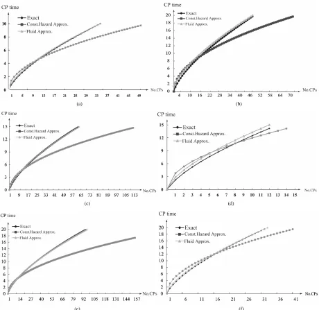
other words, the computation accuracy for two appro- ximate algorithms becomes worse as the shape parameter deviates from  1.0 more and more. In Figure 5, we investgate the dependence of the optimal aperiodic CP time on the scale parametr and the operation time in the strict IFR case. Looking at (a) to (f), only the constant hazard approximation shows the different behavior from the exact solutions.

(a)

(b)

[image:8.595.62.281.81.597.2]

(c)

Figure 3. Aperiodic CP placement with different shape pa-rameters for T = 15. (a) Case 1: γ = 0.5 and θ = 10; (b) Case 2: γ = 1.0 and θ = 10; (c) Case 3: γ = 2.0 and θ = 10.

for varying the failure parameters



 ,



when three al- gorithms are used. In the terms of approximate algo- rithms, is caluculated by substituting each ap- proximate CP sequence into Equation (5), so that

 

T N

AV t





T

AV 

and AV n_T

 

_b in Equations (26) and (29) are calculated, where ₀ 2

 

t td is used for the

k

t

k

_

n

(a)

(b)

[image:8.595.304.527.84.584.2]

(c)

Figure 4. Aperiodic CP placement with different shape pa-rameters for T = 20.(a) Case 1: γ = 0.5 and θ = 10; (b) Case 2: γ = 1.0 and θ = 10; (c) Case 3: γ = 2.0 and θ = 10.

[image:9.595.57.541.120.735.2]

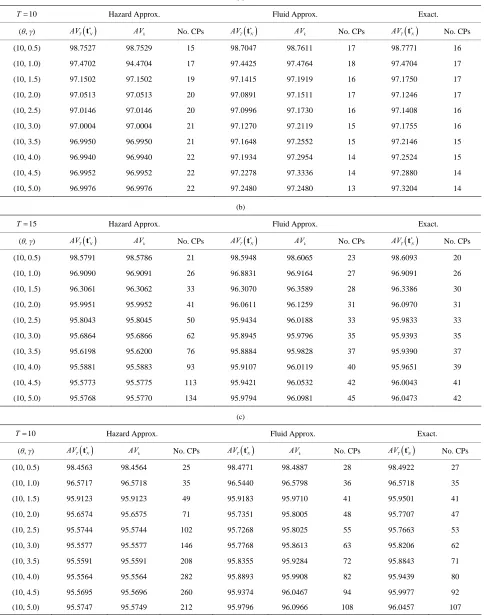
Table 1. Dependence of the shape parameter γon the steady-state system availability. (a) Case 1: T = 10; (b) Case 2: T = 15; (c) Case 3: T = 20.

(a)

10

T Hazard Approx. Fluid Approx. Exact.

(θ, γ) AVT

 

N



t AVk No. CPs AVT

 

N



t AVk No. CPs AVT

 

N



t No. CPs

(10, 0.5) 98.7527 98.7529 15 98.7047 98.7611 17 98.7771 16

(10, 1.0) 97.4702 94.4704 17 97.4425 97.4764 18 97.4704 17

(10, 1.5) 97.1502 97.1502 19 97.1415 97.1919 16 97.1750 17

(10, 2.0) 97.0513 97.0513 20 97.0891 97.1511 17 97.1246 17

(10, 2.5) 97.0146 97.0146 20 97.0996 97.1730 16 97.1408 16

(10, 3.0) 97.0004 97.0004 21 97.1270 97.2119 15 97.1755 16

(10, 3.5) 96.9950 96.9950 21 97.1648 97.2552 15 97.2146 15

(10, 4.0) 96.9940 96.9940 22 97.1934 97.2954 14 97.2524 15

(10, 4.5) 96.9952 96.9952 22 97.2278 97.3336 14 97.2880 14

(10, 5.0) 96.9976 96.9976 22 97.2480 97.2480 13 97.3204 14

(b)

15

T Hazard Approx. Fluid Approx. Exact.

(θ,γ) AVT

 

N



t AVk No. CPs AVT

 

N



t AVk No. CPs AVT

 

N



t No. CPs

(10, 0.5) 98.5791 98.5786 21 98.5948 98.6065 23 98.6093 20

(10, 1.0) 96.9090 96.9091 26 96.8831 96.9164 27 96.9091 26

(10, 1.5) 96.3061 96.3062 33 96.3070 96.3589 28 96.3386 30

(10, 2.0) 95.9951 95.9952 41 96.0611 96.1259 31 96.0970 31

(10, 2.5) 95.8043 95.8045 50 95.9434 96.0188 33 95.9833 33

(10, 3.0) 95.6864 95.6866 62 95.8945 95.9796 35 95.9393 35

(10, 3.5) 95.6198 95.6200 76 95.8884 95.9828 37 95.9390 37

(10, 4.0) 95.5881 95.5883 93 95.9107 96.0119 40 95.9651 39

(10, 4.5) 95.5773 95.5775 113 95.9421 96.0532 42 96.0043 41

(10, 5.0) 95.5768 95.5770 134 95.9794 96.0981 45 96.0473 42

(c)

10

T Hazard Approx. Fluid Approx. Exact.

(θ, γ) AVT

 

N



t AVk No. CPs AVT

 

N



t AVk No. CPs AVT

 

N



t No. CPs

(10, 0.5) 98.4563 98.4564 25 98.4771 98.4887 28 98.4922 27

(10, 1.0) 96.5717 96.5718 35 96.5440 96.5798 36 96.5718 35

(10, 1.5) 95.9123 95.9123 49 95.9183 95.9710 41 95.9501 41

(10, 2.0) 95.6574 95.6575 71 95.7351 95.8005 48 95.7707 47

(10, 2.5) 95.5744 95.5744 102 95.7268 95.8025 55 95.7663 53

(10, 3.0) 95.5577 95.5577 146 95.7768 95.8613 63 95.8206 62

(10, 3.5) 95.5591 95.5591 208 95.8355 95.9284 72 95.8843 71

(10, 4.0) 95.5564 95.5564 282 95.8893 95.9908 82 95.9439 80

[image:10.595.58.538.125.723.2]

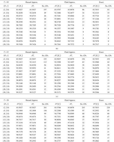
Table 2. Dependence of the scale parameter  on the steady-state system availability. (a) Case 1: T = 10; (b) Case 2: T = 15; (c) Case 3: T = 20.

(a)

10

T Hazard Approx. Fluid Approx. Exact.

 ,  AVT

 

N



t AVk No. CPs AVT

 

N



t AVk No. CPs AVT

 

N



t No. CPs

(2, 2.0) 83.5027 83.5027 197 83.5707 83.8078 86 83.7033 83 (5, 2.0) 92.2638 92.2638 49 92.3486 92.4677 34 92.4143 33 (8, 2.0) 95.6733 95.6733 26 95.7281 95.8064 21 95.7724 21 (10, 2.0) 97.0513 97.0515 20 97.0891 97.1511 17 97.1246 17 (13, 2.0) 98.2550 98.2551 14 98.2749 98.3222 13 98.3031 13 (15, 2.0) 98.7205 98.7205 12 98.7320 98.7736 11 98.7577 11 (18, 2.0) 99.1519 99.1519 10 99.1557 99.1907 9 99.1781 9 (20, 2.0) 99.3348 99.3348 9 99.3354 99.3565 8 99.3561 8 (23, 2.0) 99.5196 99.5196 8 99.5180 99.5451 7 99.5359 7 (25, 2.0) 99.6052 99.6052 7 99.5995 99.6268 6 99.6183 6 (28, 2.0) 99.6976 99.6976 6 99.6943 99.7152 6 99.7078 6 (30, 2.0) 99.7426 99.7426 6 99.7361 99.7572 5 99.7517 5

(b) 15

T Hazard Approx. Fluid Approx. Exact.

 ,  AVT

 

N



t AVk No. CPs AVT

 

N



t AVk No. CPs AVT

 

N



t No. CPs

(2, 2.0) 83.5027 83.5027 235 83.5027 83.8078 156 83.7033 152 (5, 2.0) 92.1413 92.1413 112 92.2308 92.3497 63 92.2960 62 (8, 2.0) 94.8230 94.8230 56 94.9024 94.9820 39 94.9459 39 (10, 2.0) 95.9951 95.9952 41 96.0611 96.1259 31 96.0970 31 (13, 2.0) 97.2857 97.2857 29 97.3325 97.3822 24 97.3604 24 (15, 2.0) 97.8891 97.8891 24 97.7926 97.9685 21 97.9499 21 (18, 2.0) 98.5157 98.5157 20 98.5420 98.5776 17 98.5632 17 (20, 2.0) 98.8074 98.8074 17 98.8257 98.8580 15 98.8456 15 (23, 2.0) 99.1168 99.1168 15 99.1290 99.1568 13 99.1465 13 (25, 2.0) 99.2650 99.2650 14 99.2764 99.2999 12 99.2906 12 (28, 2.0) 99.4301 99.4301 12 99.4369 99.4589 11 99.4506 11 (30, 2.0) 99.5127 99.5127 11 99.5171 99.5379 10 99.5306 10

(c)

20

T Hazard Approx. Fluid Approx. Exact.

 ,  AV

 

n



t AVk No. CPs AV

 

n



t AVk No. CPs AV

 

n



t No. CPs

(a) (b)

(c) (d)

[image:11.595.68.528.85.532.2]

(e) (f)

Figure 5. Aperiodic CP placement with different scale parameters and operation time for γ = 2.0. (a) Case 1: θ = 5 and T = 10; (b) Case 2: θ = 20 and T = 10; (c) Case 3: θ = 5 and T = 15; (d) Case 4: θ = 25 and T = 15; (e) Case 5: θ = 5 and T = 20; (f) Case 6: θ = 20 and T = 20.

expected to increse.This intuitive observation as well as the decreasing trend of the number of CPs are corect from Table 2. If we compare the minimum steady-state system availability calculated by the exact solution algo- rithm with the other ones, the relative error in both app- roximate methods can be found at the order of . Especially, the reason why the constant hazard appro- ximation works well is that it increases the number of CPs so as to increase the system availability. This im- plies that even the constant hazard approximation prob- vides the nice approximate performance on the maximum system availability. On the other hand, the number of CPs in the fluid approximation is also close to the exact

0.01%

one. Through these numerical examples, it can be con- cluded that if the steady-state system availability is evalu- ated with higher accuracy such as four or five nines, it is needed to apply the exact solution algorithms, where the initial value of the number of CPs is decided by the fluid approximation. Otherwise, i.e., the three nines level is enough for calculating the steady-state system availabi- lity, then the fluid approximation provides rather good CP schedule.

6. Conclusion

ximate algorithms to create the aperiodic checkpoint sche- dule maximizing the steady-state system availability, when the file system operation terminates at a fixed time horizon. Since the determination of the number of check- points within the finite operation-time period has been an essential problem, we have combined the fluid approxi- mation with the exact solution algorithm. In numerical ex- amples with Weibull system failure time distribution, we have calculated the optimal aperiodic checkpoint sequ- ence under different parametric circumstances. It has been shown that the combined algorithm with the fluid approximation could calculate effectively the exact solu- tions on the optimal aperiodic checkpoint sequence.

REFERENCES

[1] S. Hiroyama, T. Dohi and H. Okamura, “Comparison of Aperiodic Checkpoint Placement Algorithms,” In: G. S. Tomar, R.-S. Chang, O. Gervasi, T. H. Kim and S. K. Bandyopadhyay, Eds., Advanced Computer Science and Information (AST 2010), Communications in Computer

and Information Science, Vol. 74, Springer-Verlag, Ber- lin, 2010, pp. 145-156.

[2] V. F. Nicola, “Checkpointing and Modeling of Program Execution Time,” In: M. R. Lyu, Ed., Software Fault

Tolerance, John Wiley & Sons, New York, 1995, pp. 167-188,

[3] K. Naruse and S. Maeji, “Optimal Checkpoint Intervals for Computer Systems,” In:S. Nakamura and T. Naka- gawa, Eds., Stochastic Reliability Modeling, Optimization

and Applications, World Scientific, Singapore City, 2010, pp. 205-239.

[4] J. W. Young, “A First Order Approximation to the Opti- mum Checkpoint Interval,” Communications of the ACM, Vol. 17, No. 9, 1974, pp. 530-531.

doi:10.1145/361147.361115

[5] F. Baccelli, “Analysis of Service Facility with Periodic Checkpointing,” Acta Informatica, Vol. 15, No. 1, 1981, pp. 67-81. doi:10.1007/BF00269809

[6] K. M. Chandy, “A Survey of Analytic Models of Roll- Back and Recovery Strategies,” IEEE Computer, Vol. 8, No. 5, 1975, pp. 40-47. doi:10.1109/C-M.1975.218955 [7] K. M. Chandy, J. C. Browne, C. W. Dissly and W. R.

Uhrig, “Analytic Models for Rollback and Recovery Stra- tegies in Database Systems,” IEEE Transactions on Soft-

ware Engineering, Vol. SE-1, No. 1, 1975, pp. 100-110. doi:10.1109/TSE.1975.6312824

[8] T. Dohi, N. Kaio and S. Osaki, “Optimal Ccheckpointing and Rollback Sstrategies with Media Failures: Statistical Estimation Algorithms,” Proceedings of 1999 Pacific Rim

International Symposium on Dependable Computing (PRDC 1999), Hong Kong, 16-17 December 1999, pp. 161-168. [9] T. Dohi, N. Kaio and S. Osaki, “The Optimal Age-De-

pendent Checkpoint Strategy for a Stochastic System Subject to General Failure Mode,” Journal of Mathe-

matical Analysis and Applications, Vol. 249, No. 1, 2000, pp. 80-94. doi:10.1006/jmaa.2000.6939

[10] T. Dohi, N. Kaio and K. S. Trivedi, “Availability Models with Age Dependent-Checkpointing,” Proceedings of 21st

Symposium on Reliable Distributed Systems (SRDS 2002), Osaka, 13-16 October 2002, pp. 130-139.

[11] E. Gelenbe and D. Derochette, “Performance of Rollback Recovery Systems under Intermittent Failures,” Commu-

nications of the ACM, Vol. 21, No. 6, 1978, pp. 493-499. doi:10.1145/359511.359531

[12] E. Gelenbe, “On the Optimum Checkpoint Interval,” Jour-

nal of the ACM, Vol. 26, No. 2, 1979, pp. 259-270. doi:10.1145/322123.322131

[13] E. Gelenbe and M. Hernandez, “Optimum Checkpoints with Age Dependent Failures,” Acta Informatica, Vol. 27, No. 6, 1990, pp. 519-531. doi:10.1007/BF00277388 [14] P. B. Goes and U. Sumita, “Stochastic Models for Per-

formance Analysis of Database Recovery Control,” IEEE

Transactions on Computers, Vol. C-44, No. 4, 1995, pp. 561-576. doi:10.1109/12.376170

[15] P. B. Goes, “A Stochastic Model for Performance Evalua-tion of Main Memory Resident Database Systems,” ORSA

Journal of Computing, Vol. 7, No. 3, 1997, pp. 269-282. doi:10.1287/ijoc.7.3.269

[16] V. Grassi, L. Donatiello and S. Tucci, “On the Optimal Checkpointing of Critical Tasks and Transaction-Oriented Systems,” IEEE Transactions on Software Engineering, Vol. SE-18, No. 1, 1992, pp. 72-77.

doi:10.1109/32.120317

[17] N. Kobayashi and T. Dohi, “Bayesian Perspective of Optimal Checkpoint Placement,” Proceedings of 9th IEEE

International Symposium on High Assurance Systems En- gineering (HASE 2005), Heidelberg, 12-14 October 2005, pp. 143-159.

[18] V. G. Kulkarni, V. F. Nicola and K. S. Trivedi, “Effects of Checkpointing and Queueing on Program Perform-ance,” Stochastic Models, Vol. 6, No. 4, 1990, pp. 615- 648. doi:10.1080/15326349908807166

[19] V. F. Nicola and J. M. Van Spanje, “Comparative Analy-sis of Different Models of Checkpointing and Recovery,”

IEEE Transactions on Software Engineering, Vol. SE-16, No. 8, 1990, pp. 807-821. doi:10.1109/32.57620

[20] U. Sumita, N. Kaio and P. B. Goes, “Analysis of Effec-tive Service Time with Age Dependent Interruptions and Its Application to Optimal Rollback Policy for Database Management,” Queueing Systems, Vol. 4, No. 3, 1989, pp. 193-212. doi:10.1007/BF02100266

[21] P. L’Ecuyer and J. Malenfant, “Computing Optimal Check- pointing Strategies for Rollback and Recovery Systems,”

IEEE Transactions on Computers, Vol. C-37, No. 4, 1988, pp. 491-496. doi:10.1109/12.2197

[22] A. Ziv and J. Bruck, “An On-Line Algorithm for Check- point Placement,” IEEE Transactions on Computers, Vol. C-46, No. 9, 1997, pp. 976-985. doi:10.1109/12.620479 [23] N. H. Vaidya, “Impact of Checkpoint Latency on Over-

head Ratio of a Checkpointing Scheme,” IEEE Transac-

tions on Computers, Vol. C-46, No. 8, 1997, pp. 942-947. doi:10.1109/12.609281

ing,” Proceedings of 2004 Pacific Rim International Sym-

posium on Dependable Computing (PRDC 2004), Tahiti, 3-5 March 2004, pp. 151-158.

[25] S. Toueg and Ö. Babaoglu, “On the Optimum Checkpoint Selection Problem,” SIAM Journal of Computing, Vol. 13, No. 3, 1984, pp. 630-649. doi:10.1137/0213039

[26] N. Kaio and S. Osaki, “A Note on Optimum Checkpoint- ing Policies,” Microelectronics and Reliability, Vol. 25, No. 3, 1985, pp. 451-453.

doi:10.1016/0026-2714(85)90195-7

[27] S. Fukumoto, N. Kaio and S. Osaki, “A Study of Check- point Generations for a Database Recovery Mechanism,”

Computers & Mathematics with Applications, Vol. 24, No. 1-2, 1992, pp. 63-70.

doi:10.1016/0898-1221(92)90229-B

[28] S. Fukumoto, N. Kaio and S. Osaki, “Optimal Check- pointing Strategies Using the Checkpointing Density,”

Journal of Information Processing, Vol. 15, No. 1, 1992, pp. 87-92.

[29] Y. Ling, J. Mi and X. Lin, “A Variational Calculus Ap- proach to Optimal Checkpoint Placement,” IEEE Trans-

actions on Computers, Vol. 50, No. 7, 2001, pp. 699-707. doi:10.1109/12.936236

[30] T. Ozaki, T. Dohi, H. Okamura and N. Kaio, “Min-Max Checkpoint Placement under Incomplete information,”

Proceedings of 2004 International Conference on De- pendable Systems and Networks (DSN 2004), Florence, June 28-July 1 2004, pp. 721-730.

[31] T. Ozaki, T. Dohi, H. Okamura and N. Kaio, “Distribu- tion-Free Checkpoint Placement Algorithms Based on Min-Max Principle,” IEEE Transactions on Dependable and Secure Computing, Vol. 3, No. 2, 2006, pp. 130-140. doi:10.1109/TDSC.2006.22

[32] T. Dohi, T. Ozaki and N. Kaio, “Optimal Sequential Checkpoint Placement with Equality Constraints,” Pro-

ceedings of 2nd IEEE International Symposium on De- pendable Autonomic and Secure Computing (DASC 2006), Indianapolis, 29 September-1 October 2006, pp. 77-84.

[33] K. Iwamoto, T. Maruo, H. Okamura and T. Dohi, “Ape-riodic Optimal Checkpoint Sequence under Steady-State System Availability Criterion,” Proceedings of 2006 Asian

International Workshop on Advanced Reliability Model-ing (AIWARM 2006), Busan, 24-25 August 2006, pp. 251- 258.

[34] H. Okamura, K. Iwamoto and T. Dohi, “A Dynamic Pro- gramming Algorithm for Software Rejuvenation Sched- uling under Distributed Computation Circumstance,” Jour- nal of Computer Science, Vol. 2, No. 6, 2006, pp. 505- 512. doi:10.3844/jcssp.2006.505.512

[35] H. Okamura, K. Iwamoto and T. Dohi, “A DP-Based Optimal Checkpointing Algorithm for Realtime Appica- tions,” International Journal of Reliability, Quality and

Safety Engineering, Vol. 13, No. 4, 2006, pp. 323-340. doi:10.1142/S0218539306002288

[36] H. Okamura and T. Dohi, “Comprehensive Evaluation of Aperiodic Checkpointing and Rejuvenation Schemes in Operational Software System,” Journal of Systems and

Software, Vol. 83, No. 9, 2010, pp. 1591-1604. doi:10.1016/j.jss.2009.06.058

[37] T. Ozaki, T. Dohi and N. Kaio, “Numerical Computation Aalgorithms for Ssequential Checkpoint Placement,” Per- formance Evaluation, Vol. 66, No. 6, 2009, pp. 311-326. doi:10.1016/j.peva.2008.11.003

[38] R. E. Barlow and F. Proschan, “Mathematical Theory of Reliability,” Society for Industrial and Applied Mathe- matics, Philadelphia, 1996.

doi:10.1137/1.9781611971194

[39] K. Naruse, T. Nakagawa and Y. Okuda, “Optimal Check-ing Time of Backup Operation for a Database System,” In: T. Dohi, S. Osaki and K. Sawaki, Eds., Recent Advances

in Stochastic Operations Research, World Scientific, Sin- gapore City, 2007, pp. 131-143.

[40] K. Naruse, T. Nakagawa and S. Maeji, “Optimal Sequen- tial Checkpoint Intervals for Error Detection,” In: T. Dohi, S. Osaki and K. Sawaki, Eds., Recent Advances in Sto-