Munich Personal RePEc Archive
Theory and Applications of TAR Model
with Two Threshold Variables
Chen, Haiqiang and Chong, Terence Tai Leung and Bai,
Jushan
Xiamen University, The Chinese University of Hong Kong, Columbia
University
1 January 2012
Online at
https://mpra.ub.uni-muenchen.de/54527/
Theory and Applications of TAR Model with Two
Threshold Variables
by
Haiqiang Chen, Terence Tai-Leung Chong and Jushan Bai∗
1/1/2012
Abstract
A growing body of threshold models has been developed over the past two decades to capture the nonlinear movement of financial time series. Most of these models, however, contain a single threshold variable only. In many empirical applications, models with two or more threshold variables are needed. This paper develops a new threshold autoregressive model which contains two threshold variables. A likelihood ratio test is proposed to determine the number of regimes in the model. The fi nite-sample performance of the estimators is evaluated and an empirical application is provided.
JEL Classification: C22
Keywords: Threshold Autoregressive Model, Misspecification, Likelihood Ratio
Test, Bootstrapping.
1 Introduction
A growing body of threshold models has been developed over the past two decades to capture the nonlinear movement of financial time series. Tong (1983) develops a
∗We would like to thank Patrik Guggenberger, Guido Kuersteiner, Yongmiao Hong and the
threshold autoregressive (TAR) model and uses it to predict stock price movements. A number of new models have been proposed since the seminal work of Tong (1983), including the smooth transition threshold autoregressive model (STAR) of Chan and Tong (1986) and the functional-coefficient autoregressive (FAR) model of Chen and Tsay (1993). Tsay (1998) develops a multivariate TAR model for the arbitrage activ-ities in the security market. Dueker et al. (2007) develop a contemporaneous TAR model for the bond market.
Most of the aforementioned models, however, contain a single threshold variable only. In many empirical applications, a model with two or more threshold variables is more appropriate. For example, Leeper (1991) divides the policy parameter space into four disjoint regions according to whether monetary andfiscal policies are active or passive. Given these policy combinations, macroeconomic variables, such as real output, inflation and unemployment have different dynamics. Tiao and Tsay (1994) divide the U.S. quarterly real GNP growth rate into four regimes according to the level and sign of the past growth rate. Durlauf. and Johnson (1995) split that cross-country GDP growth rate into different regimes according to the level of per capita real GDP and literacy rate. In modelling currency crises, Sachs et al. (1996), Frankel and Rose (1996), Kaminsky (1998) and Edison (2000) argue that the occurrence of currency crises hints at the values offiscal reserves, foreign reserves and interest rate differential between home countries and the U.S.. In these examples, TAR models with multiple threshold variables can be used to describe the dynamics of different regimes.1
As the distributional theory is rather involved, no asymptotic result has been developed for TAR models with multiple threshold variables.2 This paper contributes
to the literature by developing estimation and inference procedures for TAR models with two threshold variables. Our model is applied to identify the regimes of the Hong Kong stock market. The case of Hong Kong is of interest because of its rising role as a globalfinancial center. In 2006, Hong Kong becomes the world’s second most popular place for IPO after London. In 2007, the Hong Kong stock market ranksfifth in the world, while its warrant market ranks top worldwide in terms of turnover. Using the historical prices of the Hang Seng index and the market turnover as threshold variables, our estimation shows that the stock market of Hong Kong can be classified into a high-return stable regime, a low-return volatile regime and a neutral regime.
1
Threshold model with two threshold variables can also be applied to the cross section offinancial data. For example, in the Fama and French (1992) model, one may usefirm size and book-to-market ratio as threshold variables to explain abnormal returns of a stock. Avramov et al. (2006) also sort stocks into different categories according to historical returns and liquidity level.
2A related empirical study is the nested threshold autoregressive (NeTAR) models of Astatkie et
This is different from the conventional bull-bear classification.
The remainder of the paper is organized as follows: Section 2 presents the model and discusses the estimation procedure. Section 3 derives the limiting distribution of the threshold estimators. Section 4 proposes a likelihood ratio test to determine the number of regimes. Monte Carlo simulations are conducted and the performance of the estimation procedure is evaluated in Section 5. An empirical application is provided in Section 6. Section 7 concludes the paper.
2 TAR Model with Two Threshold Variables
Consider the following TAR model with two threshold variables which classifies the observations into four regimes:
= ⎧ ⎪ ⎪ ⎪ ⎪ ⎨ ⎪ ⎪ ⎪ ⎪ ⎩
0(1)+1(1)−1+2(1)−2 +1(1)−1 +when 1≤10 2≤20
0(2)+1(2)−1+2(2)−2 +2(2)−2 + when 1≤10 2 20
0(3)+1(3)−1+2(3)−2 +3(3)−3 + when 1 10 2≤20
0(4)+1(4)−1+2(4)−2 +4(4)−4 + when 1 10 2 20
, (1)
where
= (1 2) are the threshold variables;
0 = ¡0 120
¢
∈ΩwhereΩ= [1 1]×[2 2] is a strict subset of the support of
0 is the threshold parameter vector pending to be estimated;
( = 1234) is the order in each regime;
()= (0() 1() 2() ())0 are the structural parameters and () 6=() for
some6=.3
The model is a linear AR model within each regime.4 The threshold variables1
and2 can be exogenous variables or functions of the lags of.5 Given{ }=1, our
3
Restrictions on the structural parameters can be imposed so that there are less than four regimes. For example, if(1)=(2)=(3), the model will have two regimes only.
4An empirical example of the Model (1) is Tiao and Tsay (1994)’s four-regime TAR model for
quarterly U.S. real GNP growth rates:
=
−0015−1076−1+1 −1≤−2≤0
063−1−076−2+2 −1 −2 −2≤0
0006 + 043−1+3 −1≤−2 −20
0433−1+4 −1 −20
.
In their model, the process is divided into four regimes by1 =−2 and 2 =−1−−2, and
the threshold values are set to zero. In practice, we need to estimate the threshold values.
5The model is a Self-Exciting Threshold Autoregressive (SETAR) model if the threshold variable
objective is to estimate the threshold parameters 0 and the structural parameters
(). Without loss of generality, we let = max{
1 2 3 4} and () = 0 when
= 1234. The model can be rewritten as
=
4 X
=1
Ψ()¡0¢(0()+
X
=1
()−+) (2)
where
Ψ()¡0¢is an indicator function which equals one when the threshold condition
is satisfied, and equals zero otherwise. Specifically,
Ψ(1) ¡0¢=¡1≤10 2≤02 ¢
; Ψ(2) ¡0¢=¡
1≤10 2 02 ¢
; Ψ(3) ¡0¢=¡1 10 2≤02
¢ ; Ψ(4) ¡0¢=¡1 10 2 02
¢
For analytical reasoning, it is convenient to rewrite the model (2) in the following matrix form:
=
4 X
=1
(0)()+ (3)
where
= (0 0−1 0+1)0 =
⎛ ⎜ ⎜ ⎜ ⎜ ⎝
1 −1 −2 −
1 −2 −3 −−1
1 −1 1
⎞ ⎟ ⎟ ⎟ ⎟ ⎠
(−)×(+1)
= (1 −1 −)0 for=+ 1
(0) =
n
Ψ()¡0¢Ψ(−)1¡0¢ Ψ(+1) ¡0¢o
= ( −1 +1)0
We make the following assumptions:
(1) is stationary ergodic and(4)∞
(2){}is a sequence of i.i.d. normal errors with zero mean and finite variance
2
(3) The threshold variables 1 and 2 are strictly stationary and have a
con-tinuous joint distribution(), which is differentiable with respect to both variables. Let () denote the corresponding joint density function and () =
()
. We
assume that 0 ()≤ ∞; 0 ()≤ ∞ for= 12
(1) assumes thatis stationary ergodic, which allows us to apply the law of large
number sufficient condition for (1) to hold is maxP(|
()
|)16 (2) assumes
that {} is a sequence of i.i.d. normal errors with finite second moment.7 (3)
requires the stationarity of the threshold variables. We also assume that the threshold variables are continuous with positive density everywhere, so that it is dense near 0
as the sample size increases. This assumption is needed for the consistent estimation of threshold values.
Given= (12), the conditional least square (CLS) estimator for()is defined
as
b
()() = (0())−1
0
() ( = 1234) (4)
where
() =
n
Ψ()()Ψ(−)1() Ψ(+1) ()o
The residual sum of squares is
() =||
4 X
=1
(0)()+ −
X4
=1()b
()()||2
and we define the estimator of 0 as the value that minimizes() :
b
= arg min
∈Ω () (5)
6See Chan (1993) and Hansen (1997).
7In this paper, we generalize the TAR model to the one with two threshold variables. The error
The structural estimators evaluated at the estimated threshold values are defined as:
b
()(b) = (0(b))−10(b) (6)
Appendix 2 shows the consistency of the estimators (bb()(b))
3 Limiting Distribution of (b1b2)
In this section, the asymptotic joint distribution of the least-squares estimator b
is derived under the assumption that the magnitude of change goes to zero at an appropriate rate. As pointed out by Hansen (2000), the assumption of decaying threshold effect is needed in order to obtain an asymptotic distribution of b free of nuisance parameters.8 For notational simplicity, we rewrite Model (2) as:
=(1)+
4 X
=2
(0)()+ (7)
where
(0) =
¡
0¢ (= 234) and
()=()−(1) (= 234)
For any givenwe define
()=() ( = 1234)
Observe that()0() = 0 if6= and 0()=()
0
()
Let0()=(0)we have
=
4 X
=1
0()=
4 X
=1
()
We define the following conditional moment functionals:
() =¡0|=¢ (8)
() =¡02|=¢ (9)
Let =(0) =(0). Under the assumption (2), = 2 We define
block diagonal matrices ∗ ={ } and ∗ ={ }.9 We also need the
8This approach is
first used in the literature of change points (Bai, 1997) and applied to threshold model by Hansen (2000).
following assumptions before the limiting distribution of b can be obtained. These assumptions mainly follow Hansen (1997, 2000).
(4) ()0 for all∈Ωwhere =(0) () =
³
0Ψ
()
()
´
= 1234
(5) = ((2)0 (3)0 (4)0)0 = − = (02 03 04)0−, 0 12 is a
3−dimensional constant vector and is a −dimensional constant vector for =
234.
(6)() and () are continuous at=0
(7)01∗10 02∗2 0, where 1 = (20 −04 03)0 2= (02 03−04)0
(4) is the conventional full-rank condition which excludes perfect collinearity. Ω is restricted to be a proper subset of the support of (5) assumes that the parameter change is small and converges to zero at a slow rate when the sample size is large. Under this assumption, we are able to make the limiting distribution of b free of nuisance parameters (Chan, 1993). By letting go to zero, we reduce
the rate of convergence of b from (−1) to (−1+2) and obtain a simpler
limiting distribution of b. (6) requires the moment functionals to be continuous so that one can obtain the Taylor expansion around 0 This condition excludes
regime-dependent heteroskedasticity. (7) excludes the continuous threshold model.10 Moreover,01∗1 0 and20∗20 impose the identification condition for10 and
0
2 respectively.11
Theorem 1 Under assumptions (1) to(7), we have
1−2 ¡(b1−10) (b2−20) ¢
= (1 2)
→ arg max −∞1∞−∞2∞
∙
−1
2|1|+1(|1|)− 1
2|2|+2(|2|) ¸
where
= (
(01∗1)10
2
(02∗2)20
2 )
10This paper focuses on the discontinuous threshold effect. For continuous threshold models, one
is referred to Chan and Tsay (1998).
11Note that
1 = (02 −04 03)0 measures the size of the threshold effect for the first threshold
variable1, while2= (02 03−04)0 measures the size of the threshold effect for the second threshold
variable2. When2=46= 0 and3= 0we obtain a single threshold model with only two regimes
separated by2 =02. In this case, 10 is not identified. When 2 = 0 and3 =4 6= 0we have a
and (||) is a two-sided Brownian motion on the real line defined as:
(||) =
⎧ ⎪ ⎪ ⎨ ⎪ ⎪ ⎩
Λ(−) if 0
0 if= 0
Λ() if0
Λ(),= 12, are two independent standard Brownian motions on [0∞)
Proof. See Appendix 3.
The result of Hansen (1997) is a special case of Theorem 1 with1 = 0 or 2 =
0. One can also use Theorem 1 to simulate the confidence interval of (b1b2) The
parameter ratio can be estimated by a polynomial regression or kernel regression.
See Hansen (1997, 2000).
4 Testing for and Estimation of the Threshold
To determine the number of regimes, we first consider the null hypothesis of no threshold effect:
0 :(1) =(2) =(3) =(4)
Under the null hypothesis, there is only one regime. We define a likelihood ratio test statistic as:
= max
∈Ω(−) e
2−b2() b
2() (10)
( −)e2 is the residual sum of squares under the null hypothesis, while ( −
)b2() is the residual sum of squares under the alternatives. If0cannot be rejected,
then the model is a simple AR model. Rejection of the null hypothesis suggests the existence of more than one regimes. The threshold estimator is defined as b = arg minb2() = arg max(). Since is not identified under the null hypothesis,
the asymptotic distribution of (b) is not a standard 2 Hansen (1996) shows
that the asymptotic distribution can be approximated by the following bootstrap procedure:
Let ∗ (= 1 ) be i.i.d. (01), and set ∗ = ∗. Next, we regress ∗
on = (1 ∗−1 ∗−2 ∗−) to obtain the ∗() = ( −)e
∗2−b∗2() b
∗2() and ∗ =
max∈Ω∗()
The distribution of ∗ converges weakly in probability to the distribution of
under the null hypothesis. Therefore, one can use the bootstrap value of ∗ to approximate the asymptotic null distribution of The percentage of draws where
is our bootstrapping -value. The null hypothesis will be rejected if the -value is small.
Rejection of the null hypothesis implies the presence of threshold effects. To determine the number of regimes, a general-to-specific approach is adopted. First, a three-regime model is tested against a four-regime model. Each of the following hypotheses
() 0 :(1)=(2);
() 0 :(1)=(3);
()0 :(1)=(4);
() 0 :(2)=(3);
() 0 :(2)=(4);
( ) 0 :(3) =(4)
is tested against the alternative hypothesis
1: there are four regimes.
A likelihood ratio test
(b) = (−)b
02(b)−b12(b) b
21(b) (11) is used to test these pairs of hypotheses, where (−)b20(b) is the residual sum of squares under 0, and ( −)b21(b) is the residual sum of squares under 1. A
parametric bootstrap method is applied to obtain the critical value.bis the estimated value from the unrestricted model. Let ∗ =
4 X
=1
(b(0)+P=1b()∗−)Ψ()(b) +∗,
where ∗ are i.i.d. (01) and b()0 are estimated under the restricted model. We regress∗on= (1 ∗−1 ∗−2 ∗−) to obtain∗(b) = (−)b
0∗2(b)−b∗12(b) b
∗2 1 (b)
, and
repeat this procedure a large number of times to calculate the percentage of draws for which the simulated statistic exceeds the actual value. The null is rejected if this p-value is too small.
Rejection of all the null hypotheses (I)-(VI) implies the existence of four regimes. If any one of them is accepted, then there are less than four regimes and we proceed to test a two-regime model against a three-regime model. For instance, if () 0 :
the two-regime model against the three-regime model. The following three hypotheses are tested using (b):
0 :(1) =(2) =(3);
0 :(1) =(2) =(4);
0 :(1) =(2) (3) =(4)
The alternative hypothesis is :
1 : There are three regimes with(1) =(2)
If all the above null hypotheses are rejected, we conclude that there are three regimes. Otherwise, we conclude that the model has two regimes. In empirical studies, one can estimate the autoregressive order, the threshold value and the coefficients of the TAR model via the following procedure:
Step 1: First, a first-order TAR model is estimated:
=
4 X
=1
(b0()+b1()−1)Ψ()() +b
and the initial threshold estimate b is obtained.
The first-order model is estimated for simplicity purposes (Chong, 2001). The initial threshold estimate will still be consistent even the true model is not of the
first-order (Chong, 2003; Bai et al. 2008).12
Step 2: Given the threshold values obtained from step 1, we use the AIC (Tsay,
1998) to select the autoregressive order in each regime. In our case,
() =ln[(b)] + 2( + 1) (12)
where
is the number of observations in the regime;
is the order of autoregression in the regime;
(b) is the residual sum of squares for the regime.
Define
b
= arg min ∈{12max}
() (13)
where is the maximum order considered in the model. The AIC for the
whole model can be written as
=
X
=1
(b) (14)
whereis the number of regimes.
Step 3: Perform the sequential likelihood ratio test to determine the number of
regimes.
Step 4: Use the result obtained from step 3 to refine the threshold values, and
repeat steps 2 and 3 until all the estimates converge.
5 Simulations
In the previous section, it is argued the threshold value can be consistently estimated even we start with a misspecified model in step 1. This result is obtained by Chong (2003) and Bai et al. (2008). The following experiments examine the consistency of the threshold estimator under model misspecifications.
The experiment is set up as follows: Sample size: = 200;
Number of replications: = 500;
∼(01) ∼(01) 1∼(01);
max= 10
We consider two cases for2: ()2∼(01), and () 2=1+
The following data generating processes are examined:
DGP 1 := (03−1+03−2)(1≤0 or2≤0)+(−03−1−03−2)(1
0 and 20) +;
DGP 2 := 03−1(1≤0 or 2≤0)−03−1(10 and20) +
Three misspecified models are estimated:
Model A: =
4 X
=1 b
Model B: =
4 X
=1
(b1()−1+b2()−2)Ψ()() +b;
Model C: =b1(1)−11(1≤1) +b1(2)−11(1 1) +b
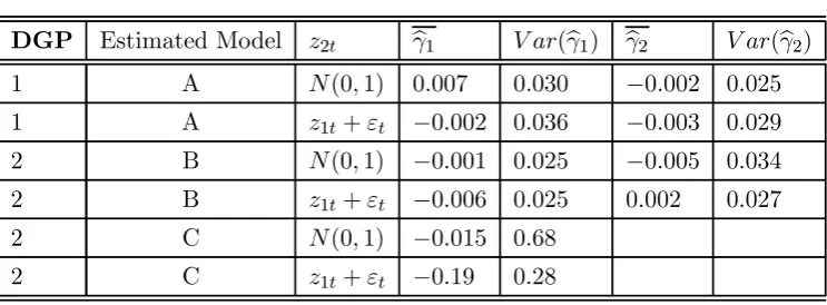
Model A underestimates the autoregressive order, while Model B overestimates the autoregressive order Both of them overestimate the number of regimes. The estimation results are reported in Table 1. For all misspecified estimated models,b1
andb2 converge to the true threshold value 0. The results for models A and B suggest
[image:13.595.121.493.401.538.2]that the consistency of the threshold estimators is unaffected by the misspecification of regressors. Therefore, if the number of threshold variables is known, one can obtain a preliminary and consistent threshold estimate using the simplest model possible. The preliminary estimate of the threshold value can be used to obtain the estimates of other parameters of interest. In the context of our model, such a preliminary threshold value allows us to determine the number of regimes, as well as the order and parameters of the autoregressive model within each regime.
Table 1: The Simulation Results
DGP Estimated Model 2 b1 (b1) b2 (b2)
1 A (01) 0007 0030 −0002 0025 1 A 1+ −0002 0036 −0003 0029
2 B (01) −0001 0025 −0005 0034 2 B 1+ −0006 0025 0002 0027
2 C (01) −0015 068 2 C 1+ −019 028
The results of Chong (2003) and Bai et al. (2008) apply to cases where the threshold variables are correctly specified. Model C underspecifies the number of threshold variables. The results for Model C show that the estimators of the single threshold-variable model may not be consistent in the presence of two dependent threshold variables.
6 Empirical Application
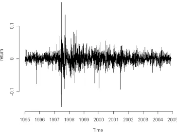
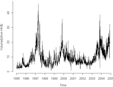
warrant market ranksfirst globally in terms of turnover. Most of the previous studies in the literature use the first lagged return as the threshold variable to identify the market regimes. Such a classification method does not take investors’ sentiment into account and does not consider the information of market turnover. In this paper, we use the past information of price and market turnover to construct our threshold variables. Our sample period runs from January 3rd 1995 to January 13th 2005. The return series is defined as the log-difference of the Hang Seng Index (HSI). There are over 2500 observations in our sample. Figure 1 and Figure 2 show the time series data for daily return and market turnover.
Figure 1 about here
Figure 2 about here
The two threshold variables are analogous to those of Granville (1963) and Lee and Swaminathan (2000). We define thefirst threshold variable as
=
20
250
(15)
where
250=
P250
=1−
250 20= P20
=1−
20
250 is the average price for the past 250 trading days;
20 is the average price for the past 20 trading days.
The variable is a ratio of two moving averages, which is similar to that of Hong and Lee (2003). In particular, the 250-day moving average, which is widely used by investors to define the market state, is employed. If the price rises above (falls below) the 250-day moving average, an average investor who has taken a long position in the previous year (about 250 trading days) has made a profit (loss), suggesting that the market sentiment should be good (bad). To reduce noise, we use the crossing of the 20-day and 250-day moving averages to help identify the market regimes.
studies have shown that the autocorrelation in stock returns is related to turnover or trading volume. For example, Campbell et al. (1993) find that the first-order daily return autocorrelation tends to decline with turnover, and the returns accompanied by high volume tend to be reversed more strongly. Llorente et al. (2002) point out that intensive trading volume can help to identify the periods in which shocks occur. Therefore, we define the second threshold variable as:
= log (−1)− −1 (16)
where
=
P250
=1log (−)
250
Figure 3 shows the two threshold variables and
Figure 3 about here
Our four-regime threshold model on the return series is
=
4 X
=1
Ψ()¡0¢(0()+(1)−1+2()−2++()−) + (17)
where
is the return series defined as the log-difference of the HSI;
Ψ(1) ¡0¢=¡
≤10 ≤20 ¢
; Ψ(2) ¡0¢=¡≤10 20
¢ ; Ψ(3) ¡0¢=¡
10 ≤20 ¢
; Ψ(4) ¡0¢=¡ 10 20
¢
The estimated threshold values from step 1 in Section 3 are: b = 102 and
b
= 057. The results of the sequential likelihood ratio test are shown in Tables 2a
[image:15.595.102.541.659.730.2]and 2b.
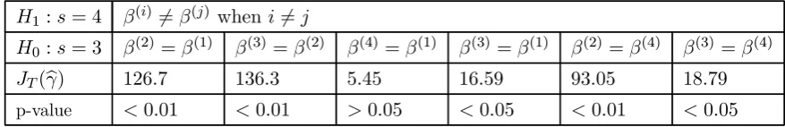
Table 2a: Results of the LR Test for 4 Regimes vs 3 Regimes
1 := 4 ()6=() when 6=
0 := 3 (2) =(1) (3) =(2) (4) =(1) (3) =(1) (2) =(4) (3) =(4)
(b) 1267 1363 545 1659 9305 1879
Note from Table 2a that the null hypothesis(4) =(1) cannot be rejected since
(b) has a p-value larger than 00513 Next, we proceed to test the 3-regime model
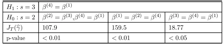
[image:16.595.118.493.193.267.2]against the 2-regime model. The results from Table 2b suggest that the movement of the return series can be approximated by a three-regime model.
Table 2b: Results of the LR Test for 3 Regimes vs 2 Regimes
1:= 3 (4) =(1)
0:= 2 (2) =(3)(4)=(1) (1)=(2)=(4) (3) =(4) =(1)
(b) 1079 1595 1877
p-value 001 001 005
Table 3 shows thefinal estimation results. The threshold estimates are revised to b
[image:16.595.109.510.376.468.2]= (102053)
Table 3: The Estimated TAR Model
Regime Estimation Results
I = 00003 + 0065−1 if102and≤053
II = 00067−03−1−04−2+018−3+009−4−012−5+054−6
−05−7−018−8 if≤102and053
III = 000014 + 0096−1 Otherwise.
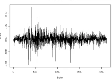
Figure 4 plots the estimated residuals of the model.14
Figure 4 about here
Using the Markov-switching model, Maheu and McCurdy (2000) divide the stock market into a high-return stable regime and a low-return volatile regime. From Table 3, we are able to classify the stock market of Hong Kong into three regimes. Since high turnover is usually associated with volatile returns (Karpoff, 1987; Foster and Viswanathan, 1995), Regime I generated by our model corresponds to the high-return
13
In some cases, if two or more hypotheses cannot be rejected, we choose the one with the largest p-value as the candidate model in the subsequent step.
14A Ljung-Box test has been conducted and the results suggest that the residuals are white noise.
stable regime, while Regime II is the low-return volatile regime.15 Regime III is a neutral regime. Table 4 shows a chronology of major events affecting the Hong Kong stock market between 1996 and 2005.16
Table 4: A Chronology of the Hong Kong Stock Market and the
Corresponding Regimes
Date Event Regime
1997.7 The establishment of the Hong Kong Special Administration Region I 1997.10.23 Asian currency turmoil triggered by thefloating of Thai Baht II 1998.1-1999.3 The burst of the property market III, II 1999.9-2000.3 Global technology stock boom and the admission of China into I, III
the WTO
2000.4-2000.6 The burst of the high-tech bubble II, III
2001.9.11 The 911 incident I
2001.11.13 The accession of China to the WTO I
2003.2-2003.6 The outbreak of SARS I, II
2003.6.29 The launch of Closer Economic Partnership Arrangement with China I
7 Conclusion
Conventional threshold models only allow for a single threshold variable. In many applications, the use of multiple threshold variables is needed. In this paper, a new
15Note that the
first-order coefficient for Regime I is 0.065, which is positive as compared to that of −03 for Regime II. This agrees with Campbell et al. (1993) that the first-order daily return autocorrelation tends to decline when turnover increases.
16We associate the estimated regimes with these major events. For example, the establishment of
TAR model with two threshold variables is developed. In addition, the consistency and limiting distribution of the estimators are established. A likelihood ratio test is also constructed to detect the threshold effect. Our model is applied to identify the regimes of the Hong Kong stock market. The two threshold variables used in this paper are analogous to those of Granville (1963) and Lee and Swaminathan (2000). Unlike the conventional bull-bear classification, it is shown that the Hong Kong stock market can be classified into three regimes, namely, a high-return stable regime, a low-return volatile regime and a neutral regime. It should be mentioned that our model assumes a single threshold for each threshold variable. It can be extended to allow for the existence of multiple thresholds (Gonzalo and Pitarakis, 2002). For example, if there are two threshold variables and each threshold variable has two threshold values, then the model can have at most nine regimes. One may also define the threshold condition as a nonlinear function of the two threshold variables. Finally, one may relax the i.i.d. assumption of the error term to allow for serial dependence and regime-dependent heteroskedasticity. Such extensions, however, are beyond the scope of this paper and are left for future research.
References
1. Amihud, Y. and H. Mendelson (1986). Asset Pricing and the Bid-Ask Spread.
Journal of Financial Economics 17, 223-249.
2. Amihud, Y. (2002). Illiquidity and Stock Returns: Cross-Section and Time Series Effects. Journal of Financial Markets5, 31-56.
3. Astatkie, T., D.G. Watts and W.E. Watt (1997). Nested Threshold Autore-gressive (NeTAR) Models. International Journal of Forecasting 13, 105-116.
4. Avramov, D., T. Chorida and A. Goyal (2006). Liquidity and Autocorrelation in Individual Stock Returns. Journal of Finance LXI, 2365-2390.
5. Bai, J., H. Chen, T.T.L. Chong and X. Wang (2008). Generic Consistency of the Break-Point Estimator under Specification Errors in a Multiple-Break Model. Econometrics Journal 11, 287-307.
6. Bai, J. (1997). Estimation of a Change Point in Multiple Regressions. Review of Economics and Statistics, 79, 551-563.
Stock Returns. Journal of Financial Economics49, 345-73.
8. Campbell, J.Y., S.J. Grossman and J. Wang (1993). Trading Volume and Serial Correlation in Stock Returns. Quarterly Journal of Economics 108, 905-939.
9. Caner M. and B.E. Hansen (2001). Threshold Autoregression with a Unit Root.
Econometrica 69, 1555-1596.
10. Chan, K.S. and H. Tong (1986). On Estimating Thresholds in Autoregressive Models. Journal of Time Series Analysis 7, 179-190.
11. Chan, K.S. (1993). Consistency and Limiting Distribution of the Least Squares Estimator of a Threshold Autoregressive Model. Annals of Statistics 21, 520-533.
12. Chen, R. and R.S. Tsay (1993). Functional-Coefficient Autoregressive Models.
Journal of the American Statistical Association 88, 298-308.
13. Chong, T.T.L. (2003). Generic Consistency of the Break-Point Estimator under Specification Errors. Econometrics Journal6, 167-192.
14. Chong, T.T.L. (2001). Structural Change in AR(1) Models. Econometric The-ory 17, 87-155.
15. Dueker, M., S. Martin and F. Spagnolo (2007). Contemporaneous Thresh-old Autoregressive Models: Estimation, Testing and Forecasting. Journal of Econometrics 141, 517-547.
16. Durlauf, S. N. and P. A. Johnson (1995). Multiple Regimes and Cross-country Growth Behavior. Journal of Applied Econometrics10, 365-384.
17. Edison, H.J. (2000). Do Indicators of Financial Crises Work? An Evaluation of an Early Warning System. Board of Governors of Federal Reserve System, International Finance Discussion Papers Number 675.
18. Foster, F.D. and S. Viswanathan (1995). Can Speculative Trading Explain the Volume-Volatility Relation? Journal of Business and Economic Statistics 13, 379-396.
19. Frankel, J.A. and A. Rose (1996). Currency Crashes in Emerging Markets: Empirical Indicators. NBER WP5437.
20. Gonzalo, J. and J. Pitarakis (2002). Estimation and Model Selection Based Inference in Single and Multiple Threshold Models. Journal of Econometrics
21. Granville, J. (1963). Granville’s New Key to Stock Market Profits, Prentice Hall.
22. Hansen, B.E. (2000). Sample Splitting and Threshold Estimation. Economet-rica 68, 575-603.
23. Hansen, B.E. (1997). Inference in TAR models. Studies in Nonlinear Dynamics and Economics 2, 1-14.
24. Hansen, B.E. (1996). Inference when a Nuisance Parameter is not Identified under the Null Hypothesis. Econometrica 64, 413-430.
25. Hong, Y. and T.H. Lee (2003). Inference on Predictability of Foreign Exchange Rate via Generalized Spectrum and Nonlinear Time Series Models. Review of Economics and Statistics85, 1048-1062.
26. Kaminsky, G.L. (1998). Currency and Banking Crises: The Early Warnings of Distress. Board of Governors of the Federal Reserve System. International Finance Discussion Papers Number 629.
27. Karpoff, J.M. (1987). The Relation between Price Changes and Trading Vol-ume: A Survey. Journal of Financial and Quantitative Analysis22,109-125.
28. Lee, M.C. and B. Swaminathan (2000). Price Momentum and Trading Volume.
Journal of Finance IV, 2017-2069.
29. Leeper, E.M. (1991). Equilibria under “Active” and “Passive” Monetary and Fiscal Policies. Journal of Monetary Economics27 129-147.
30. Llorente, G., R. Michaely, G. Saar and J. Wang (2002). Dynamic Volume-Return relation of Individual Stocks. Review of Financial Studies 15, 1005-1047.
31. Maheu, J.M. and T.H. McCurdy (2000). Identifying Bull and Bear Markets in Stock Returns. Journal of Business and Economic Statistics18, 100-112.
32. Sachs, J., A. Tornell and A. Velasco (1996). Financial Crises in Emerging Markets: The Lessons from 1995. Brookings Papers on Economic Activity No.1,
147-215.
33. Tsay, R.S. (1998). Testing and Modeling Multivariate Threshold Models. Jour-nal of the American Statistical Association 93, 231-240.
35. Tong, H. (1983). Threshold Models in Non-linear Time Series Analysis(Lecture Notes in Statistics No. 21), New York: Springer-Verlag.
Appendix 1: Lemmas
Throughout the Appendix, let||||= ((0))12 denote the Euclidean norm of a matrix Let||||= (||)1 denote the −norm of a random matrix and ⇒
denote weak convergence with respect to the uniform metric. Let= (1 −1 −2 −)0 for=+ 1 + 2 ;
= (0 0−1 0+1)(−)×(+1);
= ( +1)0;
= ( −1 +1)0;
() =
n
Ψ()()Ψ(−)1() Ψ(+1) ()o
whereΨ()() is defined in Section 2.
Let and () be moment functionals defined as:
=(0) () =
³
0Ψ
()
()
´
= 1234
Lemma 1: Under assumptions (1)−(2), it can be shown that
(a) 1
0→ ;
(b) 1
0 → 0
Proof: The proof is straightforward by applying the law of large number for
stationary ergodic processes.¥
Lemma 2: For any ∈ Ω under assumptions (1)−(3) we have, for =
1234, (a) 1 0 () →(); (b) 1 0
() → 0;
(c) 1
(
0
())0(0())
→(02Ψ
()
()) =2()
Proof: The proof of part (a) for = 1 is similar to the proof of Lemma A1
in Hansen (1996) by replacing { ≤ } with {1 ≤ 1 2 ≤ 2}. For = 2,
we have 1
0
2() =
1
X
0{1 ≤ 1}−
1
X
0{1 ≤ 1 2 ≤ 2}
→
¡0{1≤1}¢−¡0{1≤1 2≤2}¢ = 2(). Similar proof can be
Appendix 2: Consistency of Estimators
To prove the consistency of the estimatorb= arg min∈Ω (), it suffices to
show that () converges uniformly to a function () which is minimized at
0For simplicity, denoteb()=b()() for = 1234. Let b() = 4 X
=1
()b().
The residual sum of squares can be written as:
() =|| −b()||2=0 −b()0b()
=
4 X
=1 ³
()00(0)()−b()00()b()
´ + 2
4 X
=1
0(0)()+0
Next, we prove that() has a unique minimum at=0. We partition the
threshold space into four regions.
Case 1: 1 ≤10 and 2≤20
Using Lemmas 1 and 2, and the facts that
1()1(0) =1() 1()(0) = 0 for = 234;
2()1(0) =2()−2(1 20) 2()2(0) =2(1 20);
2()(0) = 0for= 34;
3()1(0) =3()−3(10 2) 3()2(0) = 0;
3()3(0) =3(01 2) 3()4(0) = 0;
4()1(0) =1(0) +1()−1(10 2)−1(1 20);
4()2(0) = 0 4()3(0) =4(10 2)−4(0) 4()4(0) =4(0);
it can be shown that
b
(1)= (01())−101() = (01())−101()[ 4 X
=1
(0)()+]
=(1)+√1
(
01()
)
−1(01()
√
)
→(1);
b
→2−1()(2()−2(1 20))((1)−(2)) +(2);
b
(3)= (0
3())−103()
→3−1()(3()−30(10 2))((1)−(2))+3−1()3(10 2)((3)−(2))+(2);
b
(4)= (0
4())−104()
→4−1()£4(0)−4(10 2)−4(1 20) +4()¤((1)−(2))
+4−1()4(0)((4)−(2)) +4−1()(4(10 2)−4(0))((3)−(2)) +(2)
Therefore,
1
(()−0)
= 1
4 X
=1 ³
()00
(0)()−b()00()b()
´ +2
4 X
=1
0
(0)()
=X4
=1 ()0
(0)(()−(2))
−hb(1)01() +b(2)0(2()−2(1 02)) i
((1)−(2)) +b(3)0[
3()−3(10 2)]((1)−(2))
+b(4)0[4(0)−4(10 2)−4(1 20) +4()]((1)−(2))
−hb(3)03(10 2) +b(4)0(4(01 2)−4(0)) i
((3)−(2))
−b(4)0
4(0)((4)−(2)) +(1)
= ((1)−(2))0[1(0)−1()−2−1()(2()−2(1 20))2
−3−1()(3()−3(10 2))2
−4−1()(4(0)−4(10 2)−4(1 20) +4())2]×((1)−(2))
+((3)−(2))0[3(0)−4−1()(4(10 2)−4(0))2
−3−1()(3(10 2))2]((3)−(2))
+((4)−(2))0£4(0)−4−1()(4(0))2¤((4)−(2)) +(1)
= ((1)−(2))0
1((1)−(2)) + ((3)−(2))02((3)−(2))
+((4)−(2))03((4)−(2)) +(1)
=1() +(1)
For any1 ≤10 and 2 ≤02it is obvious that 3 is semi-positive definite since
4() 4(0) Meanwhile, using the following results:
1(0)−1() = ³
0Ψ
(1)
()
´
=(0[Ψ
(2)
()−Ψ
(2)
(1 20) +Ψ (3)
()−Ψ
(3)
(10 2) +Ψ(4) (0)−Ψ
(4)
(10 2)
−Ψ(4) (1 20) +Ψ (4)
()])
=2()−2(1 20) +3()−3(10 2)
3(0) =4(01 2)−4(0) +3(10 2)
it can be shown that1and2are semi-positive definite. Thus,1()≥1(0) =
0, and the equation holds if and only if =0
By analogy, for the remaining three cases,
1
(()−0) =() +(1) and()≥(0) = 0 for = 234.
Define a non-stochastic function() as () for the case, we have
sup
∈Ω
|1
¡
()−0
¢
−()|=(1) (18)
Thus, () is minimized if and only if = 0. This implies that the limit of 1
() is minimized at 0. By the superconsistency of b, b() will also be
con-sistent.
Appendix 3: The Limiting Distribution of b
To derive the limiting distribution ofbfor shrinking break, we let = ((2)0 (3)0 (4)0)0 =
−0 12 = (02 03 04)0 is a 3−dimensional vector of constants. Define
b
= arg min
∈Ω () = arg min∈Ω £
()−¡0¢¤
To obtain the limiting distribution ofb, wefirst examine the asymptotic behavior of ()−¡0¢in the neighborhood of the true thresholds.
Recall from Equation (7) that the true model can be written as:
=(1)+
4 X
=2
(0)()+ =(1)+0+
where0= ((2)0
(3)
0
(4)
0 ). Let
b
() =b()(),b0()=b()(0)for= 234; b
() = (b(2)0b(3)0b(4)0)0 and b(0) = (b(2)0 0 b
(3)0
0 b (4)0
For any, define = ((2) (3) (4)). We have
b
(1)() = ((1)0
(1))−1(1)0 =(1)+((1)0(1))(1)00+((1)0(1))−1(1)0
b
(1)(0) = ((1)0
0 0(1))−10(1)0 =(1)+ (0(1)00(1))−10(1)0
Since b is a consistent estimator, we study its asymptotic behavior in the neigh-borhood of the true thresholds. Let1=10+
1−2,2=20+
1−2. By Lemmas
1 and 2,
b
(1)()−b(1)(0) = ((1)0(1))−1(1)00+((1)0(1))−1(1)0−(0(1)00(1))−10(1)0
=
4 X
=2
((1)0(1))−1(1)0(0()−())+ ((1)0(1))−1((1)0 −0(1)0)
+³((1)0(1))−1−(0(1)00(1))−1
´
0(1)0
=(
1
1−2
1
) +
µ 1
12−
1
12 
+
µ 1
1−2
1
12 
=
µ 1
1−
By the √ consistency of the OLS estimator, we have b
(1)(0)−(1) =
µ 1
12 
and
b
(1)()−(1) = ³b(1)()−b(1)(0)´+³b(1)(0)−(1)´
=
µ 1
1−
¶ +
µ 1
12 
=
µ 1
12 
(19)
Moreover, since
b
() =¡0¢−10(0+) =¡0¢−100+¡0¢−10
and
b
(0) =¡000¢−100(0+) =+¡000¢−100
we have
b
()−b(0) = ¡0¢−10(0−)+¡0¢−10−
¡
000¢−100
= ( 1
1−2− ) +
µ 1
12−
1
12 
+
µ 1
1−2−
12
=
µ 1
1−
We also have
b
(0)−=¡000¢−100 =
µ 1
12 
Therefore,
b
()− = ³b()−b(0)´+³b(0)−´
=
µ 1
1−
¶ +
µ 1
12 
=
µ 1
12 
(20)
By (19) and (20), we have,
()−¡0¢
=³ −b(1)()−
b()
´0³
−b(1)()−
b()
´
−³ −b(1)(0)− 0b(0)
´0³
−b(1)(0)− 0b(0)
´
=³ −b(1)()−b()
´0³
−b(1)()−b()
´
−³ −b(1)()−0b() ´0³
−b(1)()−0b() ´
+(1)
=−2b()0(−0) +b()0(−0)0(−0)b()
+2b()0(
−0)0(−0)(b(1)()−(1)) +(1)
=0(−0)0(−0)+ 2b()0(−0)0(−0)(b(1)()−(1))
−2b()0(
−0) + (+b())0(−0)0(−0)(b()−) +(1)
=−20(−0)0(−0)−2−0(−0)+(−12+) +(1)
=1+2+(1)
where
1 = 1−2
[(−0)]0(−0)
= 1−21
X
=+1
||
4 X
=2
0
³
Ψ()()−Ψ()¡0¢´||2 (21)
and
2 = −2−0(−0) (22)
= −2−
4 X
=2
X
=+1
0
³
Ψ()()−Ψ()¡0¢´
To examine the asymptotic behavior of ()− ¡0¢, we study the
asymptotics of1 and2We consider four different cases and provide the proof for
Case 1: 0 and 0
02
³
Ψ(2) ()−Ψ(2) ¡0¢´
=02
³
Ψ(2) (1 2)−Ψ(2) (10 2) +Ψ(2) (01 2)−Ψ(2) (10 20) ´
=0
2¡(10 ≤1 1 2 2)−(1≤10 20 ≤2 2)¢
03
³
Ψ(3) ()−Ψ(3) ¡0¢´
=03
³
Ψ(3) (1 2)−Ψ(3) (10 2) +Ψ(3) (01 2)−Ψ(3) (10 20) ´
=0
3¡−(10 ≤1 1 2≤2) +(1 10 20 ≤2 2)¢
0
4
³
Ψ(4) ()−Ψ(4) ¡0¢´
=0
4
³
Ψ(4) (1 2)−Ψ(4) (10 2) +Ψ(4) (01 2)−Ψ(4) (10 20) ´
=04¡−(10 ≤1 1 2 2)−(1 10 20 ≤2 2)¢
Summing up the three terms, we have P4
=20
³
Ψ()()−Ψ()¡0¢´
= (2−4)0(10 ≤1 1 2 2)−20(1≤10 20≤2 2)
−03(01 ≤1 1 2≤2) + (3−4)0(1 10 20≤2 2)
Since the four terms are orthogonal, by Lemma 2, we have
1
P =+1||
P4
=20
³
Ψ()()−Ψ()¡0¢´||2
→(2−4)0(2(1 2)−2(10 2))(2−4) +02((1(10 2)−1(10 20))2
+03(1(1 2)−1(10 2))3+ (3−4)0(3(10 2)−3(10 20))(3−4)
By the continuity of() around0, we can apply thefirst-order Taylor approx-imation to the moment functionals and obtain the following results:
(2−4)0(2(1 2)−2(10 2))(2−4) =|1−10|(2−4)010(2−4) +(1)
02((1(10 2)−1(10 20))2 =|2−02|02202+(1)
03(1(1 2)−1(10 2))3 =|1−10|30103+(1)
where0= ()
|=0 for= 12 and =(0|=0)
Thus,
1 =1−2
1
X
=+1
||
4 X
=2
0
³
Ψ()()−Ψ()¡0¢´||2
=1−2(|1−10|(2−4)010(2−4) +|2−20|02202
+|1−10|30103+|2−20|(3−4)020(3−4)) +(1)
=||01∗101+||20∗202+(1) (23)
where∗ ={ } 1= ((2−4)0 30)0 2 = (02(3−4)0)0
Next, we consider the asymptotic property of2 for 0 and 0:
−P
=+10
³
Ψ(2) ()−Ψ(2) ¡0¢´ 2
=−2−P
=+10
³
Ψ(2) (1 2)−Ψ(2) (10 2) +Ψ(2) (10 2)−Ψ(2) (10 20) ´
2
=−2−P
=+10((10≤1 1 2 2)−(1≤10 20≤2 2))2
⇒ −2(1()−2())2;
−P=+10
³
Ψ(3) ()−Ψ(3) ¡0¢´3
=−2−P=+10
³
Ψ(3) (1 2)−Ψ(3) (10 2) +Ψ(3) (10 2)−Ψ(3) (10 20) ´
3
=−2−P=+10(−(10≤1 1 2≤2) +(1 10 20≤2 2))3
⇒ −2(−3() +4())3;
−P
=+10
³
Ψ(4) ()−Ψ(4) ¡0¢´ 4
=−2−P
=+10
³
Ψ(4) (1 2)−Ψ(4) (10 2) +Ψ(4) (10 2)−Ψ(4) (10 20) ´
4
=−2−P=+10(−(10≤1 1 2 2)−(1 10 20≤2 2))4
⇒ −2(−1()−4())4
Summing up the three terms, we have
2 = −2− 4 X
=2
X
=+1
0
³
Ψ()()−Ψ()¡0¢´
where(·) = 1234are independent Brownian motion vectors
correspond-ing to the four disjointed regions. The covariance matrix of (·) is given by
¡(1)(1)0¢ = 10, for= 13
¡(1)(1)0¢ = 20, for= 24
where =¡02|=0¢=2 and 0 =
()
|=0 for= 12
Let 1∗() = (1()−3()) 2∗() = (−2() 4()) 1∗() and 2∗() are
two independent Brownian motion vectors with covariance matrix¡∗1(1)1∗(1)0¢=
∗0 1
¡
2∗(1)2∗(1)0¢=∗0
2 respectively, where ∗ ={ }
Thus, (24) can be rewritten as
2 ⇒ −2[1∗()(02−04 03)0+2∗()(02 03−04)0]
= −2[1∗()1+2∗()2]
= −2( q
0
1∗1101() + q
0
2∗2202()) (25)
where1() and 2() are independent standard Brownian motions.
Similarly, for the other three cases, we can show
1 =||10∗101+||20∗202+(1);
2 ⇒ −2( q
0
1∗1101() + q
0
2∗2202())
Making the change-of-variables
=
0
1∗1
(0
1∗1)210
1
=
0
2∗2
(0
2∗2)220
2
and noting01∗1=201∗1 and02∗2=202∗2, we have
()−¡0¢
→1+2
⇒ 2|1|+2|2|−221(1)−222(2)
= 2(|1|+|2|−21(1)−22(2))
Define
= (
(0
1∗1)10
2
(0
2∗2)20
The asymptotic distribution can be expressed as
1−2¡(b1−10) (b2−20) ¢
= (1 2)
⇒ arg min −∞1∞−∞1∞
∙
(1
2|1|−1(1)) + ( 1
2|2|−2(2)) ¸
= arg max −∞1∞−∞2∞
∙
(−1
2|1|+1(1)) + (− 1
2|2|+2(2)) ¸
(26)