Munich Personal RePEc Archive
Modeling choice and estimating utility in
simple experimental games
Breitmoser, Yves
EUV Frankfurt (Oder)
21 March 2012
Online at
https://mpra.ub.uni-muenchen.de/37537/
Modeling choice and estimating utility
in simple experimental games
Yves Breitmoser
∗EUV Frankfurt (Oder)
March 21, 2012
Abstract
Current experimental research seeks to estimate shape and parameterization of
utility functions. The underlying experimental games tend to be “simple” in that
best responses are salient and individual choices consistent, but the analyses
ar-rive at diverging results. I analyze how precision of estimation and robustness
of results depend on the choice models used in the analysis. Analyzing dictator
and public goods games, I find that regression models overfit drastically when
choices exhibit high precision (dictator games), that structural models with
sim-ple error structure (normal or extreme value) do not fit the curvature, and that
random behavior and random taste models do not identify social motives
ro-bustly. The choice process is captured well through the random utility model for
ordered alternatives (“ordered GEV”, Small, 1987).
JEL–Codes:C50, C72, D64
Keywords: choice models, utility function, estimation, cross validation, dictator
game, public goods game
∗I thank Friedel Bolle, and participants of IMEBE 2011 for many helpful comments, and James
1
Introduction
Experimental research in economics has led to a wide range of nowadays consensual
insights. For example, experimental subjects have social preferences (Rabin, 1993,
Levine, 1998, and subsequent work), subjects do not play strict best responses with
respect to any utility function (Rosenthal, 1989, and McKelvey and Palfrey, 1995), but
choices are fairly consistent at the individual level (e.g. Andreoni, 1995a).1 Two
in-fluential papers, Andreoni and Miller (2002) and Goeree et al. (2002), then analyzed individual choice patterns in dictator game and public goods games, respectively,
for varying tax/subsidy rates and endowments. Their results confirmed the
hypoth-esis that both social preferences and noisiness of choices shape individual decision
making—even in simple donation games, where best responses seem salient.
Current quantitative research therefore estimates social motives in relation to
econometric models specifying noisiness of choice. Such “structural models” come
in three flavors, essentially, and they differ with respect to the location of noise in the
choice process. In random behaviormodels (e.g. Fisman et al., 2007), subjects
de-viate stochastically from their individually optimal response, i.e. noise affects choice
after the determination on one’s best response. In random taste models (e.g. Cox
et al., 2007), the altruism coefficient fluctuates randomly, i.e. noise sets in prior to the
determination of the best response, and inrandom utilitymodels (e.g. Cappelen et al.,
2007), the utilities of all options are perturbed randomly (usually i.i.d.).
Conte and Moffatt (2009, 2010) and Cappelen et al. (2010a) highlight that
quan-titative results such as the estimated population weights depend on the assumed
struc-ture of choice. Arguably, such dependence contributes substantially to the disagree-ment displayed in the current literature on the social motives underlying pro-social
behavior, and thus it puts the underlying, but still unanswered question of Hey (2005)
and Loomes (2005) back onto the agenda: How should choice be modeled to robustly
identify social motives? The existing literature lacks guidance on this fundamental
question, as Card et al. (2011) discuss in detail.
In the present paper, I analyze the choice structure in dictator and public goods
games by revisiting the data of Andreoni and Miller (2002) and Goeree et al. (2002).
The objective is to understand which components of choice models improve precision
1There is further experimental research, e.g. on how choice patterns depend on circumstances
and robustness in estimating utility functions.2 The main results are that structural
models avoid significant overfitting,3 that random utility models yield qualitative
ro-bustness of identified motives across treatments, and that generalized errors to adjust
kurtosis improve both descriptive and predictive adequacy highly significantly. The
ordered GEV model (Small, 1987) has all three of these attributes, to my knowledge
currently exclusively, and indeed, its quantitative estimates are precise in-sample, it
exhibits insignificant overfitting, and the identified “social motives” (model compo-nents) are qualitatively and quantitatively robust across treatments. Guided by the
general results, however, additional models may be developed in the future.
In addition, I analyze the reliability of regression models in this context, which
relates to a second current debate. The idea is that if one is interested in quantitative estimates of treatment effects, as opposed to being interested in the underlying utility
functions as such, then one might circumvent the estimation of “deep” utility
param-eters and use regression modeling. Proponents of structural modeling argue that the
structural constraints reduce overfitting and thereby increase the quantitative
robust-ness of results in relation to say linear regression models (see e.g. Keane, 2010a,b,
Rust, 2010, and Nevo and Whinston, 2010). Proponents of non-structural modeling
argue that the assumption choice probabilities exactly take the say multinomial logit
form is ad hoc and invalid itself.
This debate, too, is one of robustness, as it concerns predictive adequacy with
re-spect to “nearby” treatment conditions. If estimates do not allow for nearby intra- or
extrapolation, they give faulty description of the underlying interdependence and
can-not be considered robust. Quantitative analyses of such robustness in game-theoretic
contexts hardly exist, however. Existing research on predictive robustness has largely focused on decision making under risk and uncertainty (see e.g. Wilcox, 2008, 2011,
and Hey et al., 2010). Two exceptions are Cappelen et al. (2011) and Blanco et al.
(2011), but the present paper is the first comparative analysis (to my knowledge).
I find that regression models overfit highly significantly if subjects choose with
high precision, which applies to dictator games in my analysis, and in this case, their
estimates are unreliable quantifications of the treatment effects and of the conditional
2Robustness and predictive adequacy will be evaluated by “k-fold cross validation” across
treat-ments: The model is fit to a subset of the treatments, evaluated on the remaining treatments, and the data set is rotated such that all observations are used exactly once in the evaluation stage.
3The difference between a model’s descriptive and predictive fits is used to measure its tendency to
choice probabilities. If subjects choose with low precision, as in public goods games
in my analysis,4 then the linear approximations in regression models suffice in the
sense that they fit as well as structural models. Even in the latter case, however,
regression models do not yield robust identification of components, and including
in-teraction terms increases overfitting in either case. In contrast, structural assumptions
prevent models from overfitting in either case, and this holds for all choice
specifi-cations in my analysis (the choice specification affects the absolute fit, of course). Thus, I conclude that structural models, and ordered GEV in particular, are preferable
to regression models in analyses of social donations.
To outline the intuition, by acknowledging the ordering of alternatives, ordered
GEV can represent probability distributions with thin peaks around the utility maxi-mizer (excess kurtosis), which prevail in high precision games, or flat peaks around
the maximizer (platykurtosis), which prevail in low precision games. Such adjustment
of kurtosis is necessary to obtain efficient estimates and can be captured similarly
with generalized normal errors in random behavior and random taste models—but it
is largely absent in the current literature (an exception is Cox et al., 2007).
Random taste models fit about as well as ordered GEV in the high-precision
dictator games, but they fail to explain choice in public goods games (low-precision
choices seem too volatile to be rationalized effectively through “taste” variation).
Re-gression and random behavior models fit about as well in public goods games, but
they either fit poorly in the high-precision dictator games (regression) or the identified
components are not robust (random behavior). Thus, explaining noisiness of choice
as purely statistical “random behavior” proves inferior to relating it to the respective
utility differences as in random utility models. Finally, the multinomial logit model of random utility does not allow adjustment of kurtosis, which implies weak levels
of goodness-of-fit, but by virtue of being a random utility model, it achieves
quali-tatively robust identification of components. Thus, all standard models have certain
strengths and weaknesses, and in relation to them, random utility with generalized
errors (ordered GEV) shares the strengths and avoids most weaknesses.
Section 2 reviews the dictator game experiment of Andreoni and Miller (2002)
and the public goods experiment of Goeree et al. (2002). Section 3 describes the
4The two experimental games are both games of social donations, but they differ with respect to
currently leading approaches to model choice in this context. Section 4 discusses the
independence of irrelevant alternatives (IIA) assumption and the ordered GEV model.
Section 5 describes the econometric approach to the analysis. Sections 6 and 7 present
and discuss the results for dictator games and public goods games, respectively.
Sec-tion 8 concludes. The supplementary material contains all parameter estimates, plots
illustrating the results, and further analysis illustrating their robustness.
2
Games and data
Dictator games and public goods games are frequently analyzed experimental games
and represent the standard frameworks to investigate “social donations.” The basic
difference between these games is that public goods games have more than one active
player. In applications, it may be difficult to distinguish between dictator games and
public goods games, however. A donation that is non-strategic in the eye of one per-son may well be a strategic contribution to a public good (the welfare of the needy) in
the eyes of another, i.e. a dictator game can turn into a public goods game depending
on who is playing it. In turn, if utilities are linear in the opponents’ payoffs, or
inde-pendent of them, then optimal contributions to (linear) public goods are indeinde-pendent
of the opponents’ contributions. In such cases, a public goods game degenerates into
nindependent dictator games. Due these cross-relations between dictator and public
goods games, I require a model of social donations to be valid in each of these games.
The data sets of Andreoni and Miller (2002) and Goeree et al. (2002) have been
selected for the analysis for three reasons. First, both of these experiments have been
designed to evaluate consistency of individual choice, which implies that they are
suited to identify the locus of noise. Second, in both experiments, each subject has to
make several decisions (eight and ten, respectively) for varying tax/subsidy rates and endowments. This allows me to separate noisy donations from altruistic donations,
and thus to identify choice parameters and utility parameters econometrically. This
is a main prerequisite for predictive accuracy. Finally, the choice sets are discrete in
both experiments and of similar cardinality (ranging from 25 to 100 choices), which
suggests that the choice structure may indeed be similar in both cases.5
5Besides, let me also note that these data sets are made readily available by the authors, either on
Table 1: Treatment parameters
(a) Dictator game parameters for payoff functions Eq. (1)
EndowmentB 40 40 60 60 75 75 60 100 Hold valueτ1 3 1 2 1 2 1 1 1
Pass valueτ2 1 3 1 2 1 2 1 1
(b) Public goods game parameters for payoff functions Eq. (4)
Group size|N| 4 2 4 4 2 4 2 2 4 2
Internal returnτI 4 4 4 2 4 4 2 4 2 4
External returnτE 2 4 6 2 6 4 6 2 6 12
Dictator games
By Andreoni and Miller’s experimental design, the dictator (player 1) can give
be-tween 0 andBtokens to player 2, and each token has valueτ1for player 1 andτ2for
player 2. Formally, 1’s choice set isS1={0,1, . . . ,B}, and the two players’ payoffs
are, for alls∈S1,
π1(s) =τ1(B−s) and π2(s) =τ2s. (1)
The three parameters τ1, τ2, and B vary between treatments,6 and overall, the
176 subjects of Andreoni and Miller made eight choices each.7 Table 1a lists the
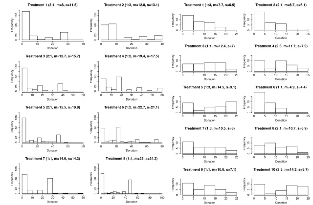
treatment parameters and Figure 1a reviews the distributions of observations. The
data exhibits typical characteristics of dictator games. For example, the donations
are fairly moderate overall, they are decreasing in τ1 and increasing in τ2. A tobit
regression of donations on(B,τ1,τ2)yields
s1=−8.172
(8.86) +(00..254066)·B−(41..348871)·τ1+4(1..878838)·τ2+ε (2)
whereεhas standard deviation ˆσ=27.645 (the standard errors are provided in
paren-theses). That is, the donation to player 2 is indeed increasing in the budget and in the donation’s value τ2 for player 2, and it is decreasing in the costs τ1 for player
6I use the term “treatment” to refer to (within subject) variation of the economic environment. 7In one session, the subjects had to make three additional choices. I discard these observations, as
1. The regression estimates suggest that the average donation falls by about 4.3 per
unit increase ofτ1 and that it increases by about 4.9 on average per unit increase of τ2. The reliability of such extrapolations is questionable, however, as it requires the
underlying model, the tobit model in this case, to have predictive accuracy.
In their analysis, Andreoni and Miller identified subjects with Cobb-Douglas,
Leontief, and linear utility functions, and with high or low precision in maximizing
utility. These utility functions are special cases of CES utilities
ui(πi,πj) =
(1−α)·(1+πi)β+α·(1+πj)β
1/β
, (3)
where(πi,πj)denotes the payoff profile. Cobb-Douglas obtains forβ→0, Leontief
forβ→ −∞, and linearity for β=1. Similar CES utility functions have been used
in most other analyses of dictator games (e.g. Fisman et al., 2007, Cox et al., 2007,
Cappelen et al., 2007, and Conte and Moffatt, 2009), and therefore my analysis will
be based on CES utilities, too.8
Public goods games
The experimental design of Goeree et al. (2002, 32 subjects and 10 treatments) varies
the group sizenof players consuming the public good as well as external returnsτE
and internal returnsτI of individual contributions. The costsτK =5 of contributions
were held constant and the choice sets areSi={0, . . . ,25}for all playersi∈N. The
payoff ofi∈Nis, for alls∈
×
i∈NSi,πi(s) =τK·(25−si) +τIsi+τE
∑
j6=isj. (4)
Table 1b and Figure 1b provide overviews of the treatment parameters and the
re-sulting choices. Again, the basic structure of contributions is fairly standard. For
example, tobit regressing contributionssion the treatment variables(N,τI,τE)yields
si=−4.721
(2.963)+(10..068515)·N+(20..5308231)·τI+0(0..80681765)·τE+ε (5)
8I useu
Figure 1: Experimental observations
Note:For each treatment, transfer ratio (τ1/τ2orτI/τE), as well as meanmand standard deviationsof choices are given in parentheses.
(a) Dictator games of Andreoni and Miller (2002)
Treatment 1 (3:1, m=8, s=11.6)
Donation
Frequency
0 10 20 30 40
0
20
60
100
Treatment 2 (1:3, m=12.8, s=13.1)
Donation
Frequency
0 10 20 30 40
0
20
60
100
Treatment 3 (2:1, m=12.7, s=15.7)
Donation
Frequency
0 10 20 30 40 50 60
0
20
60
100
Treatment 4 (1:2, m=19.4, s=17.5)
Donation
Frequency
0 10 20 30 40 50 60
0
20
60
100
Treatment 5 (2:1, m=15.5, s=19.8)
Donation
Frequency
0 20 40 60 80
0
20
60
100
Treatment 6 (1:2, m=22.7, s=21.1)
Donation
Frequency
0 20 40 60 80
0
20
60
100
Treatment 7 (1:1, m=14.6, s=14.3)
Frequency
20
60
100
Treatment 8 (1:1, m=23, s=24.2)
Frequency
20
60
100
(b) Public goods games of Goeree et al. (2002)
Treatment 1 (1:3, m=7.7, s=6.5)
Donation
Frequency
0 5 10 15 20 25
0
5
10
Treatment 2 (2:1, m=6.7, s=6.1)
Donation
Frequency
0 5 10 15 20 25
0
5
10
Treatment 3 (1:1, m=12.4, s=7)
Donation
Frequency
0 5 10 15 20 25
0
5
10
Treatment 4 (2:3, m=11.7, s=7.9)
Donation
Frequency
0 5 10 15 20 25
0
5
10
Treatment 5 (1:3, m=14.5, s=9.1)
Donation
Frequency
0 5 10 15 20 25
0
5
10
Treatment 6 (1:1, m=4.9, s=4.4)
Donation
Frequency
0 5 10 15 20 25
0
5
10
Treatment 7 (1:3, m=10.5, s=8)
Donation
Frequency
0 5 10 15 20 25
0
5
10
Treatment 8 (2:1, m=10.7, s=6.9)
Donation
Frequency
0 5 10 15 20 25
0
5
10
Treatment 9 (1:1, m=10.6, s=7.1)
10
Treatment 10 (2:3, m=14.3, s=8.7)
10
whereεhas standard deviation ˆσ=8.398. Thus, contributions are increasing in all
treatment variables, internal return, external return, and number of recipients, while
the internal return is of higher quantitative relevance than the external return (although
the external return is multiplied byN−1). In their analysis, Goeree et al. identified
players with linear and Cobb-Douglas utility functions, which further underlines the
comparability with the data of Andreoni and Miller (2002), as those again are
spe-cial cases of CES utilities. However, other studies additionally identified “conditional cooperators” (Keser and van Winden, 2000; Fischbacher et al., 2001). Such players
wish to contribute about as much as the other players contribute, i.e. their best
re-sponse functions are increasing with slope close to 1 in the opponents’ contributions.
In the present case, conditional cooperation can be modeled using Leontief
prefer-ences, and besides linear and Cobb-Douglas utilities, Leontief preferences are special
cases of then-player CES aggregator
ui=
(1−α)πβi +|Nα|−1∑j6=iπ
β
j
1/β
. (6)
Aside from the generalization of CES utilities ton-players, the main difference to the dictator game analysis will be the requirement that donations must form a strategic
equilibrium in public goods games. The usual approach in (experimental) game
the-ory is to assume that players respond to the distribution of their opponents’ choices
(following McKelvey and Palfrey, 1995, and Turocy, 2005), about which they have
rational expectations. As for public goods games, however, Goeree et al. (2002,
Foot-notes 20,21) propose that players respond to the expected contributions of the
oppo-nents, rather than their full distribution. This approach separates social preferences
and risk aversion, as players with non-linear utilities otherwise are risk averse.
Sim-ilarly, empirical studies separate social motives and risk aversion by assuming that
players respond to the actual contributions of others (e.g. of their reference group, as in Andreoni and Scholz, 1998, or the government, see Payne, 1998). For the sake of
comparability with these studies, I adopt Goeree et al.’s approach in the following.
3
Current approaches in modeling social donations
2006), while experimental studies alternatively use structural models to estimate
util-ity functions (e.g. Cappelen et al., 2007, Cox et al., 2007, and Fisman et al., 2007).
Atheoretic regression Regression models are commonly used in analyses of
dic-tator donations, and some regression models are atheoretic in that they are based on functional forms that are not derived from game-theoretic primitives such as
prefer-ence orderings and utility maximization. The model considered here regresses
dona-tions on treatment parameters (i.e. budget and transfer rates), which also constitutes
the standard approach in empirical analyses of charitable donations (see e.g. Auten
et al., 2002, and particularly recently, Bakija and Heim, 2011). Since donations in my
analysis are discrete, an interval regression with donationsias dependent variable is
required.
si=
0, if 0.5>sˆi
1, if 0.5≤sˆi<1.5
2, if 1.5≤sˆi<2.5
.. .
B, ifsi≥B−0.5
with sˆi=α+β1B+β2τ1+β3τ2+ε, (7)
andε∼
N
(0,σ2). As a second,extended regressionmodel, I will consider the modelthat additionally contains the first-order interaction terms between the treatment
vari-ables (B,τ1,τ2), i.e. B×τ1, B×τ2, and τ1×τ2. Such interactions are commonly
considered in experimental analyses, too.
Structural regression and random behavior The basic idea of random behavior
models is that players have deterministic preferences and constant best responses, but they deviate randomly when making the donation. Random behavior models have
been used for example by Fisman et al. (2007) and Conte and Moffatt (2010). A
similar model structure underlies least squares approaches, which also is used
fre-quently in the literature. Least squares relaxes the distributional assumptions on the
the error term, but it cannot be used here, as predicting the distribution of donations
is impossible without specifying the error distribution.
Formally, letu(s|α,β)denote player 1’s utility from donating s∈S1 in a
do-nation if the utility parameters are (α,β) in Eq. (3). Structural regression models
are non-linear regression models with the best response function as the deterministic
component. For the reasons discussed above, I use an interval regression with latent
variable
ˆ
si=BR(α,β) +ε. (8)
I distinguish two such models. In thestructural regressionmodel,εhas normal
dis-tribution, and in the random behavior model, ε has a generalized normal
distribu-tion (the exponential power distribudistribu-tion). The former is a fairly standard non-linear
model. I call it “structural” as the deterministic component is not a general non-linear
function, but the best response. The second model is called “random behavior” to
emphasize the behavioral component implied by the generalized error distribution.
Their joint analysis will enable us to look at the relevance of the error specification.
Random taste An alternative approach toward explaining noisiness of choice is to
allow for one’s interest in the opponent’s well-being to fluctuate randomly (Cox et al.,
2007). That is, the altruism coefficientαor “taste” is random. The key limitation of
assuming random taste is that this limits choices to those rationalizable by variations
of α. This limitation does not seem too severe in dictator or public goods games,
where variations of α seem sufficient, but in general the random taste assumption does not suffice. Formally, the donation in the random taste model is
si=BR(α+ε,β), (9)
where ε again has a generalized normal distribution. The specification used here
follows Cox et al. (2007): α′:=α/(1−α) has exponential power distribution with meanm, scales, shapeρ, i.e. density f(α′) =ρexp
(|α′−m|/s)ρ /2sΓ(1/ρ). The implied probability that i chooses an action s′i ≤si equates with F(α∗) where α∗
solvesui(si|α∗) =ui(si+1|α∗). See Cox et al. (2007, Appendix B) for illustrations.
Random utility assuming IIA The random utility model satisfying independence
of irrelevant alternatives (IIA),multinomial logit, is used very frequently in structural
op-tions fluctuate randomly. Hence players tend to deviate from the unperturbed optimal
choice but choose “better” options with higher probability. Similarly to random
be-havior, randomness of utilities may explain all deviations from utility maximization,
but now the probability of deviating to a given alternative depends on the loss that it
induces rather than its distance in the choice set.
Formally, the players are assumed to maximize ˜u(s) =λu(s|α,β) +εs overs∈
S1, withλ≥0 andεs being i.i.d. extreme value distributed (for all options s∈S1).
This distribution ofεs yields choice probabilities with the multinomial logit form and
implies IIA (Luce, 1959),
∀s∈S1: Pr(s) =eλu(s|α,β)/
∑
s′∈S
1
eλu(s′|α,β). (10)
4
Random utility without IIA
Random utility models as they are used in experimental game theory generally assume
i.i.d. random componentsεs. Examples include Anderson et al. (2001, 2002), Kübler
and Weizsäcker (2004, 2005), and Costa-Gomes et al. (2009).9 The independence of
the utility perturbations induces independence of irrelevant alternatives (IIA): when
a choices∈S1 is eliminated from the choice set S1, the relative odds between any
remaining choicess′ ands′′ are unaffected. IIA has been criticized frequently in the econometric literature, however. Tversky (1972) writes “the addition of an alternative
to an ordered set ‘hurts’ alternatives that are similar to the added alternative more
than those that are dissimilar to it,” and a similar point is made with the red bus-blue
bus example of McFadden (1973).10 General discussions of IIA can also be found in
McFadden (1976) and Samuelson (1985).
If choice sets are ordered, then similarity in Tversky’s sense may relate to the
proximity of choices. This idea has been introduced by Small (1987, 1994).11 Small’s
9This is different in other branches of economics, in particular in modeling demand functions e.g.
for residential location (McFadden, 1978), the use of telephone services (Train et al., 1987; Lee, 1999), multi-product firms (Anderson and De Palma, 1992), for urban travel (see e.g. Train, 2003, for a review), and also in modeling voting behavior (Whitten and Palmer, 1996).
10One can commute either by car or by bus, and initially, 50% of the commuters choose either
option. Now a second bus is introduced which is in all ways equivalent to the first one (and capacity constraints were never an issue). Intuitively, 50% of the commuters still choose to go by car, but under IIA, only a third of them is predicted to do so.
“ordered GEV” model essentially introduces a parameterρ∈(0,1]to capture the
cor-relation of utility perturbations between proximate choices and “weights” to capture
how correlation ceases as options become more distant. The way the model is usually
defined, stochastic independence (i.e. multinomial logit) obtains forρ=1 and perfect
correlation obtains forρ→0.
To define the model, letM∈N0denote a bandwidth parameter, and defineρ>0
and weightswm≥0 for allm=0, . . . ,Msuch that∑Mm=0wm=1. In the analysis, I use
Gaussian weights.12 The ordered GEV choice probabilities are
ω(s) =
s+M
∑
r=s
wr−sexp
λu(s|α,β)/ρ
exp{Ir}
· exp{ρIr}
∑Bt=+0Mexp{ρIt} (11)
with inclusive valueIr=ln∑s′∈Brwr−s′expλu(s′|α,β)/ρ for allr∈ {0, . . . ,B+M}
and nestsBr=
s∈ {0,1, . . . ,B} |r−M≤s≤r . That is, the player first chooses a
nestBr,r∈ {0, . . . ,B+M}, and secondly he chooses an options∈Brin this nest. The
probability of choosingsconditional on having chosenBris the first factor in each of
the summands of Eq. (11), and the probability of choosing nestBr in the first place is
the second factor above. The products of these probabilities are aggregated over all neighborhoods containings. Since every strategy belongs to M+1 nests, nests are
overlapping and the model is “cross-nested” in the sense of Vovsha (1997). Ordered
GEV also is a special case of “elimination by aspect” (Tversky, 1972), as illustrated
by McFadden (1981, p. 225f).
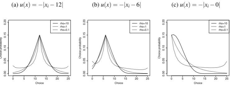
Figure 2 illustrates the choice pattern implied by varyingρin the ordered GEV
model. In general,ρ<1 implies that options with high base utility attract probability
mass away from proximate options. To see this, consider two options with perfectly
correlated utility perturbations (i.e. ρ→0). Now, the option with the higher base
utility between the two is preferred to the other one with probability one even after
perturbations. The effect is weakened but similar for allρ<1. Thus, the choice
dis-tributions haveleptokurtosis(excess kurtosis), i.e. narrow peaks and fatter tails than
nested logit model, which further illustrate that models relaxing IIA are not particularly vulnerable to overfitting. This models improve upon multinomial logit as well, but it is not as accurate as account-ing for orderaccount-ing directly (as in ordered GEV) and hence skipped for brevity.
12 That is,w
m= fN(M/2,σ2)(m)/∑Mm=0fN(M/2,σ2)(m)with free parameterσ, fN(µ,σ2) denotes the
density of the normal distribution with meanM/2 and varianceσ2. The theoretical bandwidth is set
Figure 2: Ordered GEV responses for three stylized utility functions
(a)u(x) =−|xi−12|
0 5 10 15 20 25
0.00 0.05 0.10 0.15 0.20 Choice Choice probability rho=10 rho=1 rho=0.1
(b)u(x) =−|xi−6|
0 5 10 15 20 25
0.00 0.05 0.10 0.15 0.20 Choice Choice probability rho=10 rho=1 rho=0.1
(c)u(x) =−|xi−0|
0 5 10 15 20 25
0.00 0.05 0.10 0.15 0.20 Choice Choice probability rho=10 rho=1 rho=0.1
Note:The OGEV responses, see Eq. (11), are given for choices from{0,1, . . . ,25}, with the standard deviation of the Gaussian weights (Fn. 12) being 4, the value ofρbeing as defined in the plots, and λbeing set such that the choice probability of the option maximizing base utility is 0.15 (to ensure comparability).
they display in the multinomial logit case ρ=1. Such distributions capture choice
patterns where the base utility maximizer is chosen with supra-proportional
probabil-ity but not exclusively. Arguably, such choice patterns can be expected if the utilprobabil-ity
maximizers are particularly salient. In turn,ρ>1 allows to expressplatykurtosis, i.e.
flat peaks and thin tails. Such models are not random utility models in the sense of
(McFadden, 1978), as respective choice probabilities cannot be explained by
stochas-tic utility perturbations, but they may fit choice patterns when utility maximizers are
not salient.
5
Econometric approach to the analysis
This section describes the general approach to the analysis and the two basic measures
for goodness of fit. As indicated before, both Andreoni and Miller (2002) and Goeree
et al. (2002) identified subjects with either linear, Cobb-Douglas, or Leontief utility functions, and high or low precision. Subject heterogeneity of such discrete nature
is aptly modeled as a finite mixture (McLachlan and Peel, 2000), which in turn is
standard practice in experimental analyses. For example Stahl and Wilson (1995) and
Kübler and Weizsäcker (2004) model heterogeneity in strategic reasoning as finite
mixtures, Harrison and Rutström (2009), Bruhin et al. (2010), and Conte et al. (2011)
Bardsley and Moffatt (2007) model public good contributions.
To define the finite mixture model, letK denote the set of subject types (“com-ponents”) in the population, e.g.K ={A,B,C}in a three-component population, let
(νk)k∈K denote the component shares, and for allk∈K, letPk denote the parameter
profile characterizing componentk. Now, ifoj,tdenotes thetth observation of subject
j∈Jin the data set and ifω(oj,t|Pk)is the probability that jchoosesoj,t conditional
on being of componentk, the log-likelihood of the finite mixture model is
LL(P,ν|o) =
∑
j∈J
ln
∑
k∈K
νkL(j,k) with L(j,k) =
∏
tω(oj,t|Pk). (12)
In the models estimated below, members of different components have different utility
functions and different precision in maximizing their utilities. In conjunction, these
differences encompass the different motivations for their pro-social choices. For this
reason, I will occasionally refer to the identified components as the identifiedsocial
motives.
The choice probabilitiesω(oj,t|Pk)needed to compute the likelihood follow
im-mediately from the above definitions. The model parameters are estimated by
max-imizing the likelihood function, which I maximize jointly over all parameters. This helps to avoid certain issues with two-step estimators (e.g. inconsistency and
inef-ficiency, as discussed by Amemiya, 1978, and Arcidiacono and Jones, 2003) and it
allows to extract estimates of the standard errors from the information matrix. I use
the global maximizer CMAES for the initial approach toward the maximum (an
evo-lutionary strategy, see Hansen et al., 2003, and Hansen and Kern, 2004), subsequently
the derivative-free NEWUOA algorithm (Powell, 2008) to search the wider
neighbor-hood of the initial estimates (NEWUOA is a comparably robust algorithm, see Auger
et al., 2009, and Moré and Wild, 2009), and finally a Newton-Raphson algorithm to
ensure local convergence. In order to further ensure global convergence, the above procedure had been restarted repeatedly varying the starting values.
Descriptive accuracy (model precision) Assessment of the goodness of fit of
econo-metric models are usually based on measures such as Bayes’ information criterion
BIC=−LL+d/2·lnOwith d as the number of parameters of the model andO as
the number of independent observations (the number of subjects). The termd/2·lnO
nec-essarily raise the maximum of the likelihood function (for the underlying
assump-tions, see Schwarz, 1978). In finite mixture models, this correction is insufficient and
BIC tends to overestimate the number of components. Biernacki et al. (1999, 2000)
propose to use the complete-data likelihood of the mixture model (which additionally
accounts for the likelihood of the component membership indicators) instead of the
likelihood itself to address this shortcoming. The resulting integrated classification
likelihood (ICL) criterion is derived under assumptions otherwise equivalent to those of BIC, and can be approximated by
ICL-BIC=−LL+d/2·lnO+En(τ)ˆ
with En(τ) =ˆ −
∑
j∈Jk∑
∈Kˆ
τjkln ˆτjk with τˆjk=
νkL(j,k)
∑k′∈Kνk′L(j,k′), (13)
where ˆτjk is the posterior probability of j’s membership in component k based on
the parameter estimates. The “entropy” En(τ)ˆ of the classification matrix ˆτjk
j,k
penalizes mixture models with poorly separated, thus superfluous components. I will
useICL-BIC in order to assess the goodness of fit in-sample. McLachlan and Peel
(2000, Chapter 6) discussICL-BICand alternative measures in more detail.
Predictive accuracy (model robustness) A complementary approach toward model
validation is the assessment of its predictive accuracy, as this specifically measures
the degree to which the model captures the actual data generating process. For a gen-eral discussion, let me refer to Keane and Wolpin (2007). The predictive accuracy
is especially interesting for models of social preferences, as their lack of robustness
between studies, and even within subjects (Blanco et al., 2011), is a current topic in
experimental analyses. For this reason, I analyze to which degree robustnessacross
treatmentsdepends on model choice.13
That is, I evaluate predictive accuracy by treatment-based cross validation
(Bur-man, 1989; Zhang, 1993) with non-random holdout samples (Keane and Wolpin,
2007). The data set is partitioned intoK=4 “folds” containing two/three treatments
each. I use the observations from three folds to estimate the parameters and then
13An alternative approach would consider predictions that are both across treatments and across
Table 2: Partitioning of the data sets to assess predictive accuracy
(a) Dictator game analysis
Treatments used for . . .
Training Validation
{1,2,3,4,5,7} S1={6,8}
{1,2,3,4,6,8} S2={5,7}
{1,3,5,6,7,8} S3={2,4}
{2,4,5,6,7,8} S4={1,3}
(b) Public goods analysis
Treatments used for . . .
Training Validation
{1,2,3,4,5,6,7} S1={8,9,10}
{1,2,3,4,8,9,10} S2={5,6,7}
{1,2,5,6,7,8,9,10} S3={3,4}
{3,4,5,6,7,8,9,10} S4={1,2}
compute their log-likelihood on the fourth fold to gauge their predictive accuracy. By
rotating such that each fold is used exactly once in the validation stage, and
aggregat-ing the likelihoods, I obtain thecross validation-based information criteriondenoted
LLOut. Smyth (2000) discusses cross validation in the context of mixture models.
Using P(f),ν(f)
as the parameter estimates if foldSf (f =1, . . . ,4) is left out, and
LL(·|Sf)as the log-likelihood using these estimates evaluated on foldSf, this criterion
and its in-sample counter-part is
LLOut=− 4
∑
f=1
LL P(f),ν(f)|Sf
, LLIn=− 4
∑
f=1
LL P,ν|Sf
, (14)
with(P,ν)as the whole-sample likelihood maximizers. The folds used in the analysis
are defined in Tables 2a and 2b. They are defined such that the respective holdout
samples are not “extreme” but different. For example, in the dictator game data,
with foldS3, I use 5 observations per subject for transfer rates 1 :x, x≥1, and one
observation for 2 : 1, to predict donations in case of 2 : 1 and 3 : 1.
Using cross validation, I evaluate robustness in three (partially) complementary
ways. First, qualitative robustnessobtains if no superfluous components are
identi-fied. It is assessed by comparing the number of components identified in the whole
sample with the number of components that are robust to cross validation. The
for-merin-sample optimalnumber of components is the number that minimizesICL-BIC,
while the latterout-of-sample optimalnumber of components is the smallest number
with predictive accuracyLLOutthat is not significantly improved upon atα=0.1 (this
moderate significance threshold is introduced to mildly penalize non-parsimonious
Second,quantitative robustnessis assessed by evaluating the significance of
dif-ferences between training-sample estimates and whole-sample estimates. The
possi-ble approaches to evaluate these differences vary in the data on which the significance
of differences is evaluated. I use two such approaches. On the one hand, I evaluate
the significance on the data folds left out in the respective training samples. This
yields the null hypothesisLLIn=LLOut, which is evaluated in non-nested Vuong tests
where LLIn−LLOut >0 is significant if it exceeds the BIC correction term
signif-icantly (adopting the suggestion of Vuong, 1989, Eq. 5.9). As this test evaluates a
model’s fallacy to overfit on the training samples, I refer to it asLR test of overfitting.
On the other hand, I evaluate the differences of whole-sample estimates and
training-sample estimates on the whole data set. This tests the robustness of model estimates with respect to extending the data set from the training sample to the whole
sample. The respective null hypothesis LL(P(f),ν(f)) = LL(P,ν) is evaluated (for all folds f) in Vuong testswithout BIC correction, as the parameter spaces have the
same dimensionality and the respective data sets have the same number of
indepen-dent observations. Due to dropping the BIC correction, this is a rather strict test of
quantitative robustness. I refer to it as theLR test of robustness.
6
Modeling choice in dictator games
In the next two sections, I discuss the properties of the choice models with respect
to the dictator and public goods data, respectively. The key information for dictator
games is summarized in Tables 3 and 4 below. All parameter estimates and several
illustrating plots are provided as supplementary material.
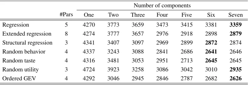
First, Table 3 provides an overview of the in-sample fit for all models with up
two seven components. Further components are not required, as the predictive
accu-racyLLout (which has been estimated simultaneously) peaks for all but the
random-utility models at five components or less, and the in-sample fitICL-BICdrops beyond
seven components for the random-utility models. This corresponds with Andreoni
and Miller (2002), who identified six distinct components in their analysis. Table 3 also lists the results of likelihood ratio tests between the models with the “in-sample
optimal” (byICL-BIC) numbers of components. I consider differences that induce
observa-Table 3: In-sample summary for the dictator games
(a) Descriptive adequacyICL-BIC=−LL+d/2·lnO+En(τˆ)(less is better)
Number of components
#Pars One Two Three Four Five Six Seven
Regression 5 4270 3773 3659 3473 3415 3381 3359
Extended regression 8 4274 3777 3657 2976 2918 2898 2879
Structural regression 3 4341 3407 3097 2969 2899 2872 2874
Random behavior 4 4337 3243 3088 2841 2686 2641 2646
Random taste 4 4316 3481 3053 2951 2713 2645 2645
Random utility 3 4724 3923 3258 3086 3042 3010 2935
Ordered GEV 4 4292 3046 2945 2846 2787 2682 2626
(b) LR tests on the descriptive adequacy using the in-sample-optimal number of components
Model 2
Model 1 CLC Regr 7 ExtReg 7 StructReg 6 RBehav 6 RTaste 6 RUtil 7 OGEV 7 Regr 7 3253.3 <<< <<< <<< <<< <<< <<<
ExtReg 7 2718.72 >>> = <<< <<< = <<<
StructReg 6 2812.38 >>> = <<< <<< = <<<
RBehav 6 2566.36 >>> >>> >>> = >> =
RTaste 6 2570.02 >>> >>> >>> = >>> =
RUtil 7 2828.68 >>> = = << <<< <<<
OGEV 7 2520.33 >>> >>> >>> = = >>>
Baseline 1 5814 <<< <<< <<< <<< <<< <<< <<<
Note: “Baseline 1” represents the prediction of uniform randomization, and otherwise, “ModelK” represents the model withKcomponents.CLC=−LL+En(τˆ)is the classification likelihood criterion. The null hypothesesH0:CLC(Model 1) =CLC(Model 2)are evaluated in Vuong LR tests accounting
for the entropies En(τˆ), and in non-nested cases also including BIC correction terms (as suggested in Eq. 5.9 of Vuong, 1989). “≫,≫, >” indicate rejection ofH0in favor of Model 1 withp< .001, .01, .1
(resp.), “≪,≪, <” indicate rejection in favor of Model 2, and “=” indicate no rejection.
tions from Table 3.
Result 6.1 (Descriptive adequacy). By their fit to the whole sample, three tiers of
models can be distinguished. First, the “advanced” structural models (random
be-havior, random taste and ordered GEV) are not significantly different at α= .01,
while all three of them fit highly significantly (p< .01) better than all other models.
Second, the basic structural models (random utility and structural regression) and
the extended regression model are not significantly different, but all of them improve
upon the final model, linear regression.
[image:20.595.99.511.150.291.2]free parameter to adjust the shape of the error distribution. The random behavior and
random taste models allow for generalized normal errors, which can have leptokurtic
shapes (thin peaks and fat tails) or platykurtic shapes (fat peaks and thin tails), and
ordered GEV allows to adjust kurtosis by varying ρ (as shown in Figure 2). Thus,
with respect to descriptive adequacy, the error specification dominates the error
lo-cation in structural models. The estimated components and utility parameters differ
between models, however, as shown in Table 5 and discussed shortly in detail, and these differences will affect robustness and predictive accuracy.
Nonetheless, these results illustrate the necessity to capture excess kurtosis in
dictator games, and to relax independence of irrelevant alternatives in these cases
(note that all three “advanced” models violate IIA). With few exceptions (e.g. Cox et al., 2007), such generalized models are not considered yet. Before discussing these
observations in further detail, let us verify their robustness out of sample (Table 4).
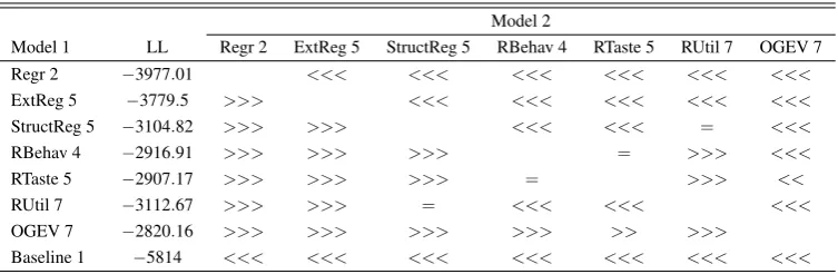
Result 6.2(Predictive accuracy). Ordered GEV fits significantly better (p< .01) than
all other models—even if we adjust their numbers of components from the in-sample
optimum to the out-of-sample optimum.14 The other two advanced structural models
still fit significantly better than random utility with IIA.
The ordered GEV model of random utility predicts most accurately. In turn,
the components identified by the other two “advanced” models, random behavior
and random taste, are less robust across treatments. In particular, the numbers of
components that remain distinct out-of-sample drop from six to four and five for
random behavior and random taste, respectively. Consequently, their out-of-sample
fit is worse than ordered GEV’s. That is, ordered GEV model does not achieve a significantly better fit in-sample, but it achieves this goodness-of-fit more robustly.
Result 6.3(Qualitative robustness). Both random utility models (multinomial logit
and ordered GEV) achieve “precise” and “robust” identification of the number of
components, i.e. the number of components identified in-sample is higher (K =7)
than those of the other structural models, and all identified components are robust to
cross validation. None of the alternative structural models yields either precision or
robustness in this sense.
14As described above,out-of-sample optimalnumber of components is the smallest number that is
Table 4: Summary of the out-of-sample analysis of dictator game models
(a) The out-of-sample log-likelihoodsLLOutEq. (14) and optimal number of components
Number of components
Model 1 1 2 3 4 5 6 7
Regr −4291.01 ≪ −3977.01 = −4292.79 < −4250.87 = −4401.51 ≪ −4354.85 ≪ −4221.45 ExtReg −4292.88 ≪ −3995.63 = −4217.06 = −4215.24 ≪ −3779.5 = −4327.79 ≪ −4272.24 StructReg −4363.7 ≪ −3403.32 < −3346.36 ≪ −3140.2 ≪ −3104.82 = −3109.03 = −3103.44 RBehav −4386.88 ≪ −3279.39 < −3231.46 ≪ −2916.91 = −2909.39 = −2919 < −2913.21 RTaste −4474.44 ≪ −3525.55 ≪ −3199.19 < −3154.33 ≪ −2907.17 = −2904.05 = −2902.23 RUtil −4830.86 ≪ −4115.95 ≪ −3537.32 ≪ −3235.43 < −3207.68 < −3192.59 ≪ −3112.67
OGEV −4333.35 ≪ −3157.81 = −3162.53 ≪ −3093.7 < −3047.88 ≪ −2872.41 ≪ −2820.16 Note:≪,≪, <indicate rejection ofH0:LLOut(k Components) =LLOut(k+1Components)withp<
.001, .01, .1. The log-likelihoodLLOutfor theout-of-sample optimalnumber of components (smallest
number of components that is not significantly improved upon atα=0.1) is set in bold-face type.
(b) Likelihood-ratio tests ofLLOutusing the out-of-sample optimal number of components
Model 2
Model 1 LL Regr 2 ExtReg 5 StructReg 5 RBehav 4 RTaste 5 RUtil 7 OGEV 7 Regr 2 −3977.01 <<< <<< <<< <<< <<< <<<
ExtReg 5 −3779.5 >>> <<< <<< <<< <<< <<<
StructReg 5 −3104.82 >>> >>> <<< <<< = <<<
RBehav 4 −2916.91 >>> >>> >>> = >>> <<<
RTaste 5 −2907.17 >>> >>> >>> = >>> <<
RUtil 7 −3112.67 >>> >>> = <<< <<< <<<
OGEV 7 −2820.16 >>> >>> >>> >>> >> >>>
Baseline 1 −5814 <<< <<< <<< <<< <<< <<< <<<
Note:“ModelK” represents the Model withKcomponents, whereKis the smallest number of com-ponents that is not significantly improved upon atα=0.1 (see Table 4a). The null hypothesis in the tests isH0:LLOut(Model 1) =LLOut(Model 2)and evaluated in Vuong tests for non-nested models;
≫,≫, >indicate rejection atp< .001, .01, .1.
(c) Likelihood-ratio tests on overfitting and robustness of parameter estimates (see Section 5)
LR tests on overfitting for number of componentsK=. . .
Model 1 1 2 3 4 5 6 7
Regr >>> > >>> >>> >>> >>> >>>
ExtReg >> > >>> >>> >>> >>> >>>
StructReg >>> >> >>> = = = =
RBehav >>> >>> = = = = =
RTaste >>> >>> >> = = > =
RUtil >>> >>> >>> = = = =
OGEV >>> = >>> = > = =
LR tests on robustness for folds . . .
S1 S2 S3 S4
Regr 7 >>> >>> >>> >>>
ExtReg 7 >>> >>> >>> >>>
StructReg 6 = = = =
RBehav 6 >>> > > =
RTaste 6 >> >> = >
RUtil 7 >> = = >>
OGEV 7 > > > >
Overfitting: H0:LLIn(Model 1) =LLOut(Model 1)evaluated in one-sided, non-nested Vuong tests (with
BIC correction term applied toLLin);≫,≫, >indicate significant overfitting at p< .001, .01, .1.
The observation that identified motives may become indistinct out of sample
would explain the lacking robustness of behavior across games currently discussed
in the literature (e.g. Blanco et al., 2011) and the lacking robustness across studies
shaping the literature. Apparently, only random utility models with or without IIA
yield qualitative robustness in dictator games such as those analyzed here.
To see why, let us next look at Table 5. It describes the identified subject types
(using the whole sample) for both in-sample and out-of-sample optimal number of
components. In all cases, strictly egoistic and strictly Leontief subjects are
identi-fied (components 1 and 2, respectively). These subjects do not deviate from utility
maximization, and hence their identification does not depend on the assumed error
structure. In the whole sample, both random behavior and random taste identified four additional components containing “noisy” players, but only two or three of them
(respectively) are robust to cross validation.
As for random behavior, the components number 4–6 in Table 5 are indistinct out-of-sample, and these components comprise 42% of the subjects. The only
sub-stantial difference between random behavior and ordered GEV is the difference in the
location of the error. Hence, this location affects the robustness. As an illustration,
consider the extreme case that a model is fitted to data for a 3 : 1 transfer ratio, i.e.
τ1 :τ2 in Eq. (1), and is used to predict data for a 1 : 1 or 1 : 3 transfer ratio.15 In
case 3 : 1, the subjective value of a token is substantially higher than in case 1 : 1,
even for altruistic subjects. As a result, the observed standard deviations differ
be-tween treatments (see also Figure 1a). Primarily, the variances of “intermediately
precise” players adapt to changes in the transfer ratios. The random behavior model
requires this subjective value to not affect the standard deviation of choices, however. Thus, it does not allow robust identification of the intermediately precise components
(numbers 4–6), which become indistinct out-of-sample.
To be more specific, Table 4c shows that the random behavior model does not predict behavior in foldS1robustly, i.e. in treatments 6 and 8 where observations have
the highest variances in absolute terms. Random utility modeling, in contrast, posits
that the probability of chosing a given option is inversely related to its opportunity
costs—and the opportunity costs depend on the transfer ratio.16 This reduces the
15The in-sample/out-of-sample ratios used in the analysis are far less extreme, see Table 2a, but the
tendency is similar.
Table 5: The components estimated by the “advanced models” for the whole sample, using either the in-sample or the out-of-sample optimal number of components
Components
Model #1 #2 #3 #4
#5 #6 #7
Random behavior
In-sample op-timal number
−0.757 10.193 0.238 0
0.251 −67.791 0.142 0
0.501 0.49 0.175 35.3
0.347 0.174 0.16 10.9 0.49 −30.759
0.123 27.4
0.097 0.296 0.161 9.1 Out-of-sample
optim. number
−0.89 9.586 0.239 0
0.303 −86.109 0.153 0.2
0.501 0.488 0.191 34.7
0.298 0.407 0.417 14.5
Random taste
In-sample op-timal number
−0.93 29.431 0.238 0
1.229 −62.287 0.154 4.4
0.999 0.485 0.124 29.3
0.5 0.847 0.176 32.2 0.338 −0.035
0.235 18.8
0.322 0.444 0.073 8.8 Out-of-sample
optim. number
−0.381 4.927 0.238 0
1.018 −55.579 0.154 4.5
0.999 0.485 0.123 29.2
0.5 0.845 0.185 32 0.34 −0.013
0.3 18.4
Ordered GEV
In+Out −00.769 −0.045
.25 0
0.291 −79.613 0.142 0
0.5 0.491 0.083 12.7
0.331 −100 0.129 22.2 0.237 −0.374
0.069 10.9
0.361 1.043 0.186 21.6
0.081 0.37 0.141 13.3
Note: For each model and component, a matrix
α β
ν σ
is given;α,βare the CES parameters,νis the component’s weight, andσis the standard deviation of its member’s choices in treatment 8. The remaining information for all models and all numbers of components are supplementary material.
significance of violating quantitative robustness in relation to random behavior, and
in the case of ordered GEV to ap-value greater than the threshold .01.
Briefly, note that the relationship between random utility and random behavior is
inverted for the plain models with standard error specification (structural regression and multinomial logit). As for structural regression, restricting errors to be normal
improves qualitative robustness (five components out-of-sample instead of four) and
avoids significant violations of quantitative robustness for all folds. This corresponds
with the previous discussion, as restricting errors to be normal decreases the degrees
of freedom in fitting purely statistical patterns, which increases robustness, albeit
ro-bustness at a comparably weak goodness-of-fit overall. As for multinomial logit, the
restriction to extreme value perturbations restricts the goodnes-of-fit in all
dimen-sions, including predictive accuracy. This suggests that the generalized extreme value
As for random taste models, the reason for the lacking robustness is a little
dif-ferent. By construction, the model relates the choice pattern to utility differences,
albeit to differences in utility parameters rather than utilities itself. Hence, it adapts
to variations of opportunity costs and violates parametric robustness in fold S1 less
significantly than random behavior. Random taste models do not allow to fit “weak
Leontief” subjects, however, i.e. component 4 for ordered GEV in Table 5. Weak
Leontief subjects choose noisily around the minimax choice, withβ<−50 in their utility functions (1−α)πβi +απβj)1/β. If β<−50, however, the weightsα are
ir-relevant,17 and hence the noisiness of weak Leontief subjects cannot be explained
by variations ofα. In this sense, random taste models are behaviorally incomplete
and their approximation of weak Leontief subjects is not robust out-of-sample. As
Table 5 shows, these weak Leontief subjects are approximated in-sample by
compo-nent number 6, which is indistinct from compocompo-nent 5 (weak Cobb-Douglas)
out-of-sample. This failure to fit weak Leontief choices is quantitatively significant when the
random taste model has to predict behavior in foldsS1 andS2 (see Table 4c), where
the Leontief choices are more pronounced than in the other treatments.
The observation that random behavior and random taste models fail to accurately
fit parts of the choice pattern does not imply that these models overfit significantly in
relation what is expected by the BIC correction. The degree of overfitting is the
dif-ferenceLLIn−LLOut, and I consider it significant if it exceeds the BIC correction term
significantly (Vuong, 1989, Eq. 5.9). Using this criterion, the amount of overfitting is
insignificant for all structural models (Table 4c).
Result 6.4(Overfitting). Not one of the structural models overfits significantly (p< .01) if the number of components is chosen adequately (K≥4).
This confirms that the structural models do not overfit in excess of the amount
that is to be expected by adding further parameters. In random behavior and random
taste models, the added components tend to become imprecise and indistinct
out-of-sample, but they are not systematically wrong. This differs in the case of atheoretic regression, as discussed shortly, and confirms the conjecture voiced in the literature
(Keane, 2010a; Rust, 2010) that structural modeling largely prevents overfitting—
very much in contrast to atheoretic modeling.
The required dimensionalityK≥4 is predicated byICL-BICin-sample and thus
17Note that (1−α)πβ i +απ
β
known without cross validation. In addition it is intuitive. It allows for the two
ponents with high-precision utility maximizers, egoistic and Leontief, for one
com-ponent with low-precision members (comcom-ponent 3 in the random behavior model has
standard deviation of 35, see Table 5), and for one component with intermediate
pre-cision (type 4 in the random behavior model has standard deviation 15 out of sample).
Nonetheless, the observation that overfitting is insignificant forallstructural models
with at least this dimensionality deserves emphasis. It suggests that six observations per subject suffice to train the structural models, although the parameter space in the
analyzed structural models has a dimensionality that would be considered high by
most standards (up to 35 parameters for 176×8 observations).
Finally, the following result summarizes the main observations on the two athe-oretic regression models.
Result 6.5(Atheoretic regression). The linear regression models overfit highly
signif-icantly and improvements of the in-sample fit—achieved by adding either interaction
terms or mixture components—are not robust to treatment-based cross validation.
Apparently, the descriptive accuracy achieved by linear (atheoretic) regression
is misleading in the analyzed dictator games. This again confirms the conjecture
voiced in the literature. The reason is rather obvious: The non-linearity of the
best-response functions in most treatment parameters (in all parameters but endowment
E, that is) cannot be approximated by linear functions and interactions. Since most
subjects tend to maximize utility indeed, as shown by Andreoni and Miller (2002),
their precision is too high to be approximated linearly. While the choice patterns seem
to be captured reasonably well in-sample, although worse than with the advanced structural models, the predictions are systematically off the mark out-of-sample. In
particular, regression models fail to predict the location of the second mode in the
empirical distributions, i.e. the choices made by the high-precision Leontief subjects.
These systematic mistakes, in turn, imply the significance of overfitting. Having said
7
Modeling choice in public goods games
Analyses of public goods games based on random utility models are fairly common
in the experimental literature, but always under the premise that IIA is satisfied.18
Thus, it will be interesting to see how relevant the above observation that IIA need
be relaxed to capture excess kurtosis proves to be in this context. Random behavior
modeling was used by Bardsley and Moffatt (2007), and only they account for
sub-ject heterogeneity by finite mixture modeling. In turn, random taste models or GEV models are not considered in the existing literature.
The following analysis comprises mixture models with up to four components,
as the out-of-sample fitLLOut drops beyond three components for all but the random
utility models, and ICL-BIC drops beyond four components for the random utility
models (details on this are provided in the supplementary material). The basic
(athe-oretic) regression model regresses contributions on treatment parameters again (group
size, external return, and internal return), while the extended regression model
addi-tionally includes interaction terms. Table 6 summarizes the in-sample fit for all
mod-els and Table 7 describes their out-of-sample fit.19 The main results on the in-sample
fit are summarized first.
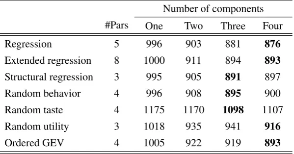
Result 7.1(Descriptive accuracy). There are three tiers of models again. First,
re-gression, random behavior, and ordered GEV fit about similarly well (none of them
fits significantly worse than any other of them atα=.01). Second, multinomial logit fits significantly worse than ordered GEV, and lastly, random taste does not fit.
Similarly to modeling dictator game choices, the ability to adjust kurtosis in re-lation to multinomial logit proves important, as implied by the significance of the
difference between multinomial logit and ordered GEV. Contrary to above, the fitted
distributions tend to be platykurtic rather than leptokurtic for about 70% of the
sub-jects, i.e. they exhibit flatter peaks and thinner tails. This corresponds loosely with
ρ=10 in Figure 2. Ordered GEV models withρ>1 do not satisfy the sufficient con-dition for being random utility models (McFadden, 1978), however. Intuitively, the
18For example, multinomial logit was applied by Anderson et al. (1998) to standard public goods
games, by Offerman et al. (1998), Myatt and Wallace (2008), and Choi et al. (2008) to threshold public goods games, and by Willinger and Ziegelmeyer (2001) and Yi (2003) to nonlinear games.
19Again, the supplementary material contains all parameter estimates and plots showing that the
Table 6: In-sample summary for public goods games
(a) Goodness of fitICL-BIC=−LL+d/2·lnO+En(ˆτ)(less is better)
Number of components
#Pars One Two Three Four
Regression 5 996 903 881 876
Extended regression 8 1000 911 894 893
Structural regression 3 995 905 891 897
Random behavior 4 996 908 895 900
Random taste 4 1175 1170 1098 1107
Random utility 3 1018 935 941 916
Ordered GEV 4 1005 922 919 893
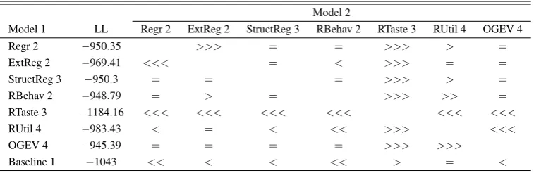
(b) Likelihood-ratio tests using the in-sample-optimal number of components
Model 2
Model 1 CLC Regr 4 ExtReg 4 StructReg 3 RBehav 3 RTaste 3 RUtil 4 OGEV 4
Regr 4 835.67 = = = >>> > =
ExtReg 4 832.2 = = = >>> = =
StructReg 3 872.23 = = = >>> = =
RBehav 3 871.03 = = = >>> = =
RTaste 3 1073.97 <<< <<< <<< <<< <<< <<<
RUtil 4 876.04 < = = = >>> <<<
OGEV 4 852.74 = = = = >>> >>>
Baseline 1 1043 <<< <<< <<< <<< >>> <<< <<<
H0:LL(Model 1) =LL(Model 2)with>>>, >>, >indicatingp≤.001, .01,0.1 in favor of Model 1.
For a detailed description, see Table 3b.
flatness of the peaks implies that deviations from the utility maximizer are
compara-tively likely, i.e. precision is low. The probability of remote choices has to be
propor-tional, though, while the fitted choice probabilities actually drop supra-proportionally
outside the neighborhood of the utility maximizer.
From a more general point of view, platykurtic choice patterns suggest that
sub-jects have an idea of their utility maximizer and randomize fairly uniformly over its
neighborhood. The corresponding two thirds of the subjects (withρ≈10) are
there-fore closer to random behavior than random utility. The more relevant observation
is, however, that ordered GEV offers the flexibility required to capture such choice
patterns (by allowing forρ>1). Thus, although it does not improve upon the explicit random behavior models with respect to goodness-of-fit here, it provides a general
(multinomial logit) and the random taste model cannot capture these behavioral
pat-terns. In particular, rationalizing choices by adjusting the altruism coefficientα in
cases where the utility maximizer is not sufficiently salient proves econometrically
ineffective.20
Another difference to dictator games is that the linear approximation used in
regression models seems adequate here. Arguably, the reason is the previous
obser-vation that the utility maximizer is not salient, which implies that noise is comparably
high and that choice patterns can be approximated linearly without much loss. To
quantify the noisiness of choices, let us look at the hypothetical model that predicts
the actually observed relative frequencies in all treatments. It would score a
log-likelihood of−787 and a pseudo-R2 of 0.245. The corresponding pseudo-R2 in the dictator game data is 0.579. That is, the upper bar for the descriptive accuracy is
rather low to begin with. In relation to this upper benchmark of−787, in turn, the
in-sample likelihood−850 of ordered GEV is good. In order to ultimately assess the
fit of atheoretic regression, let us look at the out-of-sample results next (Table 7).
Result 7.2(Predictive accuracy). All three modeling approaches (atheoretic
regres-sion, random behavior, and random utility) are in principle predictive. However,
multinomial logit predicts significantly worse than ordered GEV, and the extended
regression model (which includes interaction terms) predicts significantly worse than
the plain regression model. None of these models overfits systematically (atα=.01)
if the number of components is chosen appropriately (i.e. to minimize ICL-BIC).
Thus, in contrast to dictator games, linear approximations suffice in-sample and
do not overfit more than predicted by the BIC correction term. The number of
pa-rameters of the extended model is rather large, however, and thus its BIC correction
is large. Indeed, the model without interaction terms fits significantly better than the
extended model out-of-sample, and in this sense, the extended model does overfit.
Further, in absolute terms, the regression models overfit slightly more than the struc-tural models, i.e. random behavior and ordered GEV.
Finally, let us look at the robustness of the identified components again.
20To be more precise, strict rationalization of all choices by varying altruism is ineffective, because
the general amount of noise is too high. To see this, compute theα′=α/(1−α)that explain the mean
observations in the various treatments. The ratio of the highestα′to the lowestα′required is 3.08 in