ISSN Online: 2161-7198 ISSN Print: 2161-718X
DOI: 10.4236/ojs.2017.74039 Jul. 31, 2017 567 Open Journal of Statistics
Sparse Additive Gaussian Process with Soft
Interactions
Garret Vo
1, Debdeep Pati
21Department of Industrial and Manufacturing Engineering, Florida State University, Tallahassee, FL, USA 2Department of Statistics, Texas A and M University, College Station, TX, USA
Abstract
This paper presents a novel variable selection method in additive nonparame-tric regression model. This work is motivated by the need to select the number of nonparametric components and number of variables within each nonpa-rametric component. The proposed method uses a combination of hard and soft shrinkages to separately control the number of additive components and the variables within each component. An efficient algorithm is developed to select the importance of variables and estimate the interaction network. Ex-cellent performance is obtained in simulated and real data examples.
Keywords
Additive, Gaussian Process, Interaction, Lasso, Sparsity, Variable Selection
1. Introduction
Variable selection has played a pivotal role in scientific and engineering applications, such as biochemical analysis [1], bioinformatics [2] and text mining [3], among other areas. A significant portion of existing variable selection methods are only applicable to linear parametric models. Despite the linearity and additivity assumption, variable selection in linear regression models has been popular since 1970, referring to Akaike information criterion (AIC; [4]); Bayesian information criterion (BIC; [5]) and Risk inflation criterion (RIC; [6]).
Popular classical sparse-regression methods such as Least absolute shrinkage operator (LASSO [7] [8]), and related penalization methods [9] [10] [11] [12] have gained popularity over the last decade due to their simplicity, computational scalability and efficiency in prediction when the underlying relation between the response and the predictors can be adequately described by parametric models. How to cite this paper: Vo, G. and Pati, D.
(2017) Sparse Additive Gaussian Process with Soft Interactions. Open Journal of Sta- tistics, 7, 567-588.
https://doi.org/10.4236/ojs.2017.74039
Received: June 13, 2017 Accepted: July 28, 2017 Published: July 31, 2017
Copyright © 2017 by authors and Scientific Research Publishing Inc. This work is licensed under the Creative Commons Attribution International License (CC BY 4.0).
http://creativecommons.org/licenses/by/4.0/
DOI: 10.4236/ojs.2017.74039 568 Open Journal of Statistics Bayesian methods [13] [14] [15] with sparsity inducing priors offer greater applicability beyond parametric models and are a convenient alternative when the underlying goal is in inference and uncertainty quantification. However, there is still a limited amount of literature which seriously considers relaxing the linearity assumption, particularly when the dimension of the predictors is high. Moreover, when the focus is on learning the interactions between the variables, parametric models are often restrictive since they require very many parameters to capture the higher-order interaction terms.
Smoothing based non-additive nonparametric regression methods [16] [17] [18] [19] can accommodate a wide range of relationships between predictors and response leading to excellent predictive performance. Such methods have been adapted for different methods of functional component selection with non- linear interaction terms: component selection and smoothing operator (COSSO; [20]), sparse addictive model (SAMS; [21]) and variable selection using adaptive nonlinear interaction structure in high dimensions (VANISH; [22]). However, when the number of variables is large and their interaction network is complex, modeling each functional component is highly expensive.
Nonparametric variable selection based on kernel methods is increasingly becoming popular over the last few years. Liu et al. [23] provided a connection between the least square kernel machine (LKM) and the linear mixed models. Zou et al. [24], Savitsky et al. [25] introduced Gaussian process with dimension- specific scalings for simultaneous variable selection and prediction. Yang et al. [26] argued that a single Gaussian process with variable bandwidths can achieve the optimal rate in estimation when the true number of covariates s O
(
logn)
. However, when the true number of covariates is relatively high, the suitability of using a single Gaussian process is questionable. Moreover, such an approach is not convenient to recover the interaction among variables. Fang et al. [27] used the nonnegative Garotte kernel to select variables and capture interaction. Though these methods can successfully perform variable selection and capture the interaction, non-additive nonparametric models are not sufficiently scalable when the dimension of the relevant predictors is even moderately high. [27] claimed that extensions to additive models may cause over-fitting issues in capturing the interaction between variables (i.e. capture more interacting variables than the ones which are influential).To circumvent this bottleneck, Yang et al. [26], Qamar and Tokdar [28] introduced the additive Gaussian process with sparsity inducing priors for both the number of components and variables within each component. The additive Gaussian process captures interactions among variables, can scale up to moderately high dimensions and are suitable for low sparse regression functions. However, the use of two component sparsity inducing prior forced them to develop a tedious Markov chain Monte Carlo algorithm to sample from the posterior distribution.
DOI: 10.4236/ojs.2017.74039 569 Open Journal of Statistics soft interactions. More specifically, we decompose the unknown regression function F into k components, such as F= φ1 1f + φ2 2f ++ φk kf , for k hard shrinkage parameters φ =l, 1, ,l k , k≥1. Each component fl is independent. Each of them is assigned to a Gaussian process prior. To induce sparsity within each Gaussian process, we introduce an additional level of soft shrinkage parameters. The combination of hard and soft shrinkage priors makes our approach very straightforward to implement and computationally efficient, while retaining all the advantages of the additive Gaussian process proposed by Qamar and Tokdar [28]. We propose a combination of Markov chain Monte Carlo (MCMC) and the Least Angle Regression algorithm (LARS) to select the Gaussian process components and variables within each component.
The rest of the paper is organized as follows. Section2 presents the additive Gaussian process model. Section 3 describes the two-level regularization and the prior specifications. The posterior computation is detailed in Section 4 and the variable selection and interaction recovery approach are presented in Section 5. The simulation study results are presented in Section 6. A couple of real data examples are considered in Section 7. We conclude with a discussion in Section 8.
2. Additive Gaussian Process
For observed predictor-response pairs
(
,)
p i yi ∈ ×x , where i=1,2, , n
(i.e.n is the sample size and p is the dimension of the predictors), an additive nonparametric regression model can be expressed as
( )
(
)
( )
( )
( )
( )
2
1 1 2 2
, ~ 0,
.
i i i i
i i i k k i
y F
F f f f
σ
φ
φ
φ
= + Ν
= + + +
x
x x x x (1)
The regression function F in (1) is a sum of k regression functions, with the relative importance of each function controlled by the set of non-negative
parameters
(
)
T1, , ,2 k
φ= φ φ φ . Typically the unknown parameter
φ
is assumed to be sparse to prevent F from over-fitting the data.Gaussian process (GP) [29] provides a flexible prior for each of the component functions in
{
f ll, =1, , k}
. GP defines a prior on the space of allcontinuous functions, denoted f ~ GP ,
(
µ c)
for a fixed function µ:p→ and a positive definite function c defined on
p×
p such that for any finite collection of points{
xi,i=1, , L}
, the distribution of{
f( )
x1 , , f( )
xL}
is multivariate Gaussian with mean{
µ( )
x1 , , µ( )
xL}
and variance-covariance matrix Σ ={
c(
x xi, i′)
}
1 , ,≤i i L′≤ . The choice of the covariance kernel is crucial toensure the sample path realizations of the Gaussian process are appropriately smooth. A squared exponential covariance kernel c
(
x x, ′)
=exp(
−κ x x− ′2)
with an Gamma hyperprior assigned to the inverse-bandwidth parameterκ
DOI: 10.4236/ojs.2017.74039 570 Open Journal of Statistics bandwidth parameter might be inadequate and dimension specific scalings with appropriate shrinkage priors are required to ensure that the posterior distribution can adapt to the unknown dimensionality. However, Yang et al. [26] showed that single Gaussian process might not be appropriate to capture interacting variables and also does not scale well with the true dimension of the predictor space. In that case, an additive Gaussian process is a more effective alternative which also leads to interaction recovery as a bi-product. In this article, we work with the additive representation in (1) with dimension specific scalings (inverse-bandwidth parameters) κlj along dimension j for the lth Gaussian process component,
j
=
1, ,
p
andl
=
1, ,
k
.We assume that the response vector y=
(
y y1, , ,2 yn)
in (1) is centered and scaled. Let fl~ GP 0,(
cl)
with(
)
(
)
21
, exp p .
l lj j j
j
c κ x x
= ′ = − − ′
∑
x x(2) In the next section, we discuss appropriate regularization on
φ
and{
κlj,l=1, , ; k j=1, , p}
. A shrinkage prior on the{
κlj,j=1, , p}
facilitates the selection of variables within component l and allows adaptive local smoothing. An appropriate regularization onφ
allows F to adapt to the degree of additivity in the data without over-fitting.3. Regularization
A full Bayesian specification will require placing prior distribution on both
φ
andκ
. However, such a specification requires tedious posterior sampling algorithms to sample from the posterior distribution as seen in [28]. Moreover, it is difficult to identify the role of φl and κjl,j=1, , p since one can remove the effect of the lth component by either setting φl to zero or by having0, 1, ,
lj j p
κ = = . This ambiguous representation causes mixing issues in a full-blown MCMC. To facilitate computation, we adopt a hybrid approach between frequentist and Bayesian to regularize
φ
and κlj, respectively. The hybrid-algorithm is a combination of i) MCMC, to sampleκ
conditional onφ
ii) and optimization to estimateφ
conditional onκ
. With this viewpoint, we propose the following regularization onκ
andφ
. With the parameterγ
, each component controls the selection of variables and interaction among them. In addition toγ
, the parameter Γ allows the model (1) to select significantcomponents, which includes interested variables and interaction network. Together, Γ and
γ
are the global-local shrinkage on F.3.1.
L
1Regularization for
φ
Conditional on f1, , fk, (1) with φl, and φ >l 0. Hence we impose L1
regularization on φl, which is as following
( )
( )
1 1 1
1 N k k
i l l i l
i l l
y x f x
n = =
φ
λ φ
= − +
∑
∑
∑
DOI: 10.4236/ojs.2017.74039 571 Open Journal of Statistics In the algorithm, φl is updated using least absolute shrinkage and selection operator (LASSO) [7] [32] [33]. The L1 regularization enforces sparsity on
φ
at each stage of the algorithm, thereby pruning the unnecessary Gaussian process components in F. The parameter
λ
in (3) is selected using five fold cross validation.3.2. Choice of
k
Components
The proposed model has the number of components, k, which determines how many components to fit the data and build the prediction. We propose using LASSO to choose k. First, we start with a large k value. As φj is updated with the LASSO algorithm, the LASSO algorithm prunes unnecessary Gaussian process fl. Therefore, the value of k is updated, which is equal to the number of components which are not pruned.
3.3. Global-local shrinkage for
κ
ljThe parameters κlj controls the effective number of variables within each component. For each l,
{
κlj,j=1, , p}
are assumed to be sparse. As opposed to the two component mixture prior on κlj in [28], we enforce weak-sparsity using a global-local continuous shrinkage prior which potentially have substantial computational advantages over mixture priors. Many continuous shrinkage priors have been proposed recently [34]-[39]. These priors can be unified through a global-local (GL) scale mixture representation of [40] below,(
)
~ N 0, , ~ g, ~ ,l lj lj l l f lj f
κ ψ τ τ ψ
(4) for each fixed l, where fg and fl are densities on the positive real line. In (4), τl controls global shrinkage towards the origin while the local parameters
{
ψlj,j=1, , p}
allow local deviations in the degree of shrinkage for each predictor. Special cases include Bayesian lasso [34], relevance vector machine [35], normal-gamma mixtures [36] and the horseshoe [37] [38] among others. Motivated by the remarkable performance of horseshoe, we assume both fg and fl to be square-root of half-Cauchy distributions. Bothl
τ and ψlj will be updated using the MCMC algorithm.
4. Hybrid Algorithm for Prediction, Selection
and Interaction Recovery
In this section, we develop a fast algorithm which is a combination of L1
optimization and conditional MCMC to estimate the parameters φl, ψlj, and l
τ for
l
=
1, ,
k
andj
=
1, ,
p
. Conditional on κlj, (1) is linear in φl and hence we resort to the least angle regression procedure [8] with five fold cross validation to estimate φ =l,l 1, , k. The computation of the lasso solutions is aquadratic programming problem, and can be tackled by standard numerical analysis algorithms.
DOI: 10.4236/ojs.2017.74039 572 Open Journal of Statistics special structure of the lasso problem, and provides an efficient way to compute the solutions. Next, we describe the conditional MCMC to sample from κlj and
( )
*F x at a new point
x
* conditional on the parametersl
φ . For two collection of vectors Xv and Yv of size m1 and m2 respectively, denote by
(
v, v)
c X Y
the m m1× 2 matrix
{
c x y(
,)
}
x X y Y∈ v,∈v. Let X={
x x1, , ,2 xn}
and define(
,)
,(
*,) (
, , *)
c X X c x X c X x and c
(
x x*, *)
denote the corresponding matrices. For a random variable q, we denote by q|− the conditional distribution of q given the remaining random variables.Observe that the algorithm does not necessarily produce samples which are approximately distributed as the true posterior distribution. The combination of optimization and conditional sampling is similar to stochastic EM [41] [42] which is employed to avoid computing costly integrals required to find maximum likelihood in latent variable models. Conditional on φ =l, 1, ,l k, the MCMC
algorithm to update ψlj, τl, and φl is as following:
1) Compute the kernel k x x
( )
, , k x x(
, *)
, k x x(
*,)
, k x x(
*, *)
with the kernel formula(
,)
exp(
2)
dj
k x x′ = −γ x x− ′ . 2) Compute fl
( )
i j lφj jf( )
i .−
≠ =
∑
x x Compute the predictive mean
(
)
(
)
1(
)
* *, , 2
l k c I y fl
µ = +σ − − −
x x X X
(5)
3) Compute the predictive variance
(
) (
)
(
)
1(
)
* *, * *, , 2 , * .
l c c c σ c
−
Σ = x x − x X X X + X x (6)
4) Sample | , ~ N
(
*, *)
l l l
f − y µ Σ . 5) Compute the predictive
( )
* * * *1 1 2 2 k k.
F x =φ f +φ f ++φ f
(7)
6) Update ψlj by sampling from the following posterior distribution,
(
lj| ,)
pψ − y
(
)
(
)
(
)
( )
T 2 1
2 1 exp , 2 | , . , lj lj
y c I y
p y p
c I σ ψ ψ σ − − + − ∝ + X X X X (8)
7) Update τl,j=1, , k by sampling from the following posterior distribution,
(
l| ,)
p τ − y
(
)
(
)
(
)
( )
T 2 1
2 1 exp , 2 | , . , l l
y c I y
p y p
c I σ τ τ σ − − + − ∝ + X X X X (9)
8) Update γdj by using the formula γdj = Ψτj dj. 9) Update the vector Γ with the LASSO estimation.
10) Update κlj by sampling
(
)
~ N 0, lj lj l
κ ψ τ
DOI: 10.4236/ojs.2017.74039 573 Open Journal of Statistics 11) Update φj and prune unnecessary fj where j l≠ with the LASSO algorithm.
The MCMC algorithm above is illustrated with the following flow-chart.
In the MCMC algorithm above, the conditional distributions of τj and ψlj are not available in closed form. Therefore, we sample them using Metropolis- Hastings algorithm [43]. In this paper, we give the algorithm for updating τl only, as the steps for ψlj are similar. Assuming that the chain is currently at the iteration t, the Metropolis-Hastings algorithm to sample t1
l
τ + independently for
1, ,
l
=
k
proceeds as following: 1) Propose log ~*(
log ,t 2)
l N l τ
τ τ σ .
2) Compute the Metropolis ratio:
(
)
(
)
*|
min ,1
| l t l
p p
p
τ
τ
−
=
−
DOI: 10.4236/ojs.2017.74039 574 Open Journal of Statistics 3) Sample u~ U 0,1
( )
. Ifu p
<
then log t1 log *l l
τ+ = τ , else log t1 log t
l l
τ+ = τ . The flowchart for the above Metropolis-Hastings algorithm is as following:
The proposal variance 2 τ
σ is tuned to ensure that the acceptance probability is between 20% - 40%. We also propose a similar Metropolis-Hastings algorithm to sample from the conditional distribution of ψ −lj| .
5. Variable Selection and Interaction Recovery
for Selected Variables
In this section, we first state a generic algorithm to select important variables based on the samples of the parameter vector
γ
. This algorithm is independent of the prior forγ
and unlike other variable selection algorithms, it requires few tuning parameters making it suitable for practical purposes. The idea is based on finding the most probable set of variables in the median of theγ
samples. Since the distribution for the number of important variables is more stable and largely unaffected by the Metropolis-Hastings algorithm, we find the mode H of the distribution for the number of important variables. Then, we select the H largest coefficients from the posterior mean ofγ
.In this algorithm, we use k-means algorithm [44] [45] with k=2 at each
DOI: 10.4236/ojs.2017.74039 575 Open Journal of Statistics signals h( )t is estimated by the smaller cluster size out of the two clusters. We take the mode over all the iterations to obtain the final estimate H for the
number of non-zero signals i.e. H mode=
( )
h( )t . The H largest entries of theposterior median of γ are identified as the non-zero signals.
We run the algorithm for 5000 iterations with a burn-in of 2000 to ensure convergence. Based on the remaining iterates, we apply the algorithm to κjl for each component fl to select important variables within each fl for
1, ,
l
=
k
. Using this approach, we select the important variables within each function. We define the inclusion score of a variable as the proportion of functions (out of k) which contains that variable. Next, we apply the algorithm toφ
and select the important functions. Let us denote by Af the set of active functions, obtained from the LASSO algorithm as discussed in Section 3.2. The interaction score between a pair of selected variables is defined as the proportion of functions within Af in which the selected pair appears together. Using these interaction scores, we can find the interaction between important variables with optimal number of active components. Observe that the inclusion and interaction scores are not a functional of the posterior distribution and is purely a property of the additive representation. Hence, we do not require the sampler to converge to the posterior distribution. As illustrated in Section 6, these inclusion and the interaction scores provide an excellent representation of a variable or an interaction being present or absent in the model. An illustratfor both variable selection and interaction will be displayed in Section 6.6. Simulation Examples
In this section, we consider eight different simulation settings with 50 replicated datasets each and test the performance of our algorithm with respect to variable selection, interaction recovery, and prediction. To generate the simulated data, we draw xij~ Unif 0,1
( )
, and ~ N(
( )
, 2)
i i
y f x σ , where
1
≤ ≤
i n
,1
≤ ≤
j p
and σ =2 0.02. Table 1 and Table 2 summary the result and signal to noise
ratio (SNR) for the eight different datasets with different combinations of p and n for both non-interaction and interaction cases, respectively.
6.1. Variable Selection
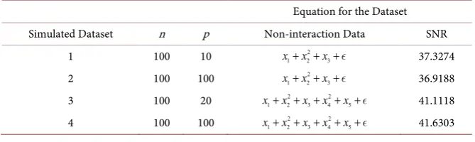
[image:9.595.206.541.629.729.2]We compute the Inclusion score for each variable in each simulated dataset, then provide the bar plots as in Figures 1-4 below.
Table 1. Non-interaction simulated datasets.
Equation for the Dataset Simulated Dataset n p Non-interaction Data SNR
1 100 10 2
1 2 3
x x x+ + + 37.3274
2 100 100 2
1 2 3
x x x+ + + 36.9188
3 100 20 2 2
1 2 3 4 5
x x x x x+ + + + + 41.1118
4 100 100 2 2
1 2 3 4 5
DOI: 10.4236/ojs.2017.74039 576 Open Journal of Statistics
Table 2. Interaction simulated datasets.
Equation for the Dataset
Simulated Dataset n p Interaction Data SNR
1 100 10 2
1 2 3 1 2 2 3 3 1
x x x x x x x x x+ + + + + + 41.9095
2 100 100 2
1 2 3 1 2 2 3 3 1
x x x x x x x x x+ + + + + + 42.1258
3 100 20 2 2
1 2 3 4 5 1 2 2 3 3 4
x x x x x x x x x x x+ + + + + + + + 43.0888
4 100 100 2 2
1 2 3 4 5 1 2 2 3 3 4
[image:10.595.207.541.337.445.2]x x x x x x x x x x x+ + + + + + + + 44.4024
[image:10.595.206.542.475.574.2]Figure 1. Inclusion score for dataset 1. (a) Non-interaction Case; (b) Interaction Case.
[image:10.595.210.538.606.702.2]Figure 2. Inclusion score for dataset 2. (a) Non-interaction Case; (b) Interaction Case.
Figure 3. Inclusion score for dataset 3. (a) Non-interaction Case; (b) Interaction Case.
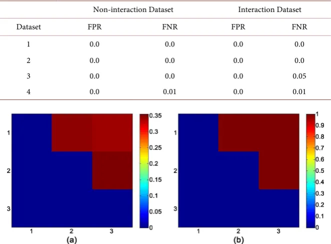
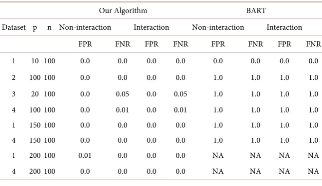
DOI: 10.4236/ojs.2017.74039 577 Open Journal of Statistics From these histograms, we rank the Inclusion score value. Based on our ranking, we select a threshold value to identify the signal based on the top Inclusion score values. From our ranking, the selected threshold value is 0.1. The ranking of variables selection has been mentioned in Guyon and Elisseeff [46], Forman [47], Stoppiglia et al. [48]. The choice of the threshold variable based upon the data has been mentioned in Genuer et al. [49]. When we obtain selected variables, we compute the false positive rate (FPR), which is the proportion of true signals not detected by our algorithm, and false negative rate (FNR), which is the proportion of false signals detected by our algorithm. Both values are recorded in Table 3 to assess the quantitative performance of our algorithm.
Based on the results in Table 3, it is immediate that the algorithm is very successful in delivering accurate variable selection for both non-interaction and interaction cases.
6.2. Interaction Recovery
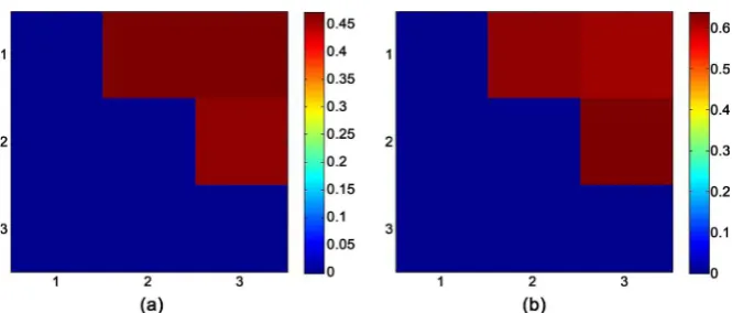
In order to capture the interaction network, we compute the probability of interaction between two variables by calculating the proportion of functions in which both the variables jointly appear. Since we are interested in capturing the interaction between selected variables, we plot interaction heat map for selected variables with their probability of interaction values, for each dataset for both the non-interaction and interaction cases.
[image:11.595.208.539.461.705.2]Based on Figures 5-8, it is evident that the estimated interaction probabilities for the non-interacting variables are less than the corresponding number for interacting variables. With these heat map values, we plot the interaction
Table 3. The average false positive (FPR) and false negative (FNR) for replicated datasets.
Non-interaction Dataset Interaction Dataset
Dataset FPR FNR FPR FNR
1 0.0 0.0 0.0 0.0
2 0.0 0.0 0.0 0.0
3 0.0 0.0 0.0 0.05
[image:11.595.207.538.464.703.2]4 0.0 0.01 0.0 0.01
DOI: 10.4236/ojs.2017.74039 578 Open Journal of Statistics
[image:12.595.206.541.239.377.2]Figure 6. Interaction heat map for dataset 2. (a) Non-interaction Case; (b) Interaction Case.
Figure 7. Interaction heat map for dataset 3. (a) Non-interaction Case; (b) Interaction Case.
Figure 8. Interaction heat map for dataset 4. (a) Non-interaction Case; (b) Interaction Case.
network in Figure 9 & Figure 10 for selected variables.
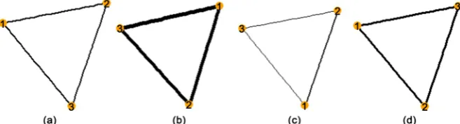
Based on the interaction network in Figure 9 & Figure 10, we observe that edges for interaction cases are thicker than edges for non-interaction cases. In interaction cases, interacted variables are connected in the network, while every variables is connected in non-interaction cases. Therefore, our algorithm successfully captures the interaction network in all the datasets for selected variables according to the Inclusion score.
6.3. Predictive Performance
[image:12.595.207.542.406.543.2]DOI: 10.4236/ojs.2017.74039 579 Open Journal of Statistics observations. We apply our algorithm on the training data and compare the performance on the test dataset. For the sake of brevity we plot the predicted vs. the observed test observations only for a few cases in Figure 11.
From Figure 11, the predicted observations and the true observations fall very closely along the
y x
=
line demonstrating a good predictive performance. We [image:13.595.209.538.205.294.2]compare our results with [27]. However, their additive model was not able to capture higher order interaction and thus have a poor predictive performance compared to our method.
[image:13.595.211.537.336.429.2]Figure 9. Interaction network for dataset 1 and 2, respectively. (a) Non-interaction 1; (b) Interaction 1; (c) Non-interaction 2; (d) Interaction 2.
Figure 10. Interaction network for dataset 3 and 4, respectively. (a) Non-interaction 3; (b) Interaction 3; (c) Non-interaction 4; (d) Interaction 4]
[image:13.595.209.539.468.678.2]DOI: 10.4236/ojs.2017.74039 580 Open Journal of Statistics
6.4. Comparison with BART
Bayesian Additive Regression Tree (BART; [50]) is a state of the art method for variable selection in nonparametric regression problems. BART is a Bayesian “sum of tree” framework which fits and infers the data through an iterative back-fitting MCMC algorithm to generate samples from a posterior. Each tree in BART [50] is constrained by a regularization prior. Hence BART is similar to our method which also resorts to back-fitting MCMC to generate samples from a posterior.
Since BART is well-known to deliver excellent prediction results, its performance in terms of variable selection and interaction recovery in high- dimensional setting is worth investigating. In this section, we compare our method with BART in all the three aspects: variable selection, interaction recovery and predictive performance. For comparison, with BART, we used the same simulation settings as in Table 1 with all combinations of (n, p), where
100
n
=
andp
=
10,20,100,150,200
.We used 50 replicated datasets and compute average inclusion probabilities for each variable. Similar to §6.1, we ranked the Inclusion score, and chose the threshold value equal to 0.1 in order to find selected variables. Then, we computed the false positive and false negative rates for both algorithms as in Table 3. These values are recorded in Table 4.
In Table 4, the first column indicates which equations are used to generate the data with the respective p and n values in the second and third column for both non-interaction and interaction cases. For example, if the dataset is 1, the equations to generate the data is 2
1 2 3
x x+ +x + and 2
1 2 3 1 2 2 3 3 1
x x+ +x +x x +x x +x x + for non-interaction and interaction case, respectively. NA value means that the algorithm cannot run at all for that particular combination of p and n values.
According to Table 4, BART performs similar to our algorithm when
p
=
10
and
n
=
100
. However, as p increases, BART fails to perform adequately while [image:14.595.207.538.538.729.2]our algorithm still performs well even when p is larger than n. When p is twice
Table 4. Comparison between our algorithm and BART for variable selection.
Our Algorithm BART
DOI: 10.4236/ojs.2017.74039 581 Open Journal of Statistics as n, BART fails to run while our algorithm provides excellent results in variable selection. Overall, our algorithm performs significantly better than BART in terms of variable selection.
7. Real Data Analysis
In this section, we demonstrate the performance of our method in two real data sets. We use the Boston housing data and concrete slump test datasets obtained from UCI machine learning repository. Both data have been used extensively in the literature.
7.1. Boston Housing Data
In this section, we used the Boston housing data to compare the performance between BART and our algorithm. The Boston housing data [51] contains information collected by the United States Census Service on the median value of owner occupied homes in Boston, Massachusetts. The data has 506 number of instances with thirteen continuous variables and one binary variable. The data is split into 451 training and 51 test observations. The description for each variable is summarized in Table 5.
MEDV is chosen as the response and the remaining variables are included as predictors. We ran our algorithm for 5000 iterations and the prediction result for both algorithms is shown in Figure 12.
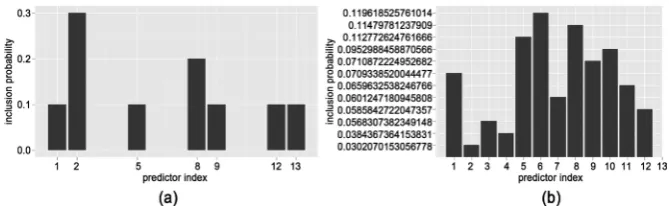
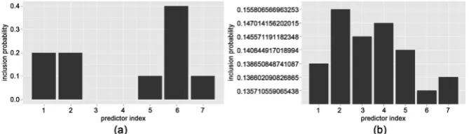
[image:15.595.194.531.463.734.2]Although our algorithm has a comparable prediction error with BART, we argue below that we have a more convincing result in terms of variable selection. We displayed the Inclusion score barplot in Figure 13.
Table 5. Boston housing Dataset variable.
Variables Abbreviation Description 1 CRIM Per capita crime rate
2 ZN Proportion of residential land zoned for lots over 25,000 squared feet 3 INDUS Proportion of non-retail business acres per town
4 CHAS Charles River dummy variable (= 1 if tract bounds river; 0 otherwise) 5 NOX Nitric oxides concentration (parts per 10 million)
6 RM Average number of rooms per dwelling
7 AGE Proportion of owner-occupied units built prior to 1940 8 DIS Weighted distances to five Boston employment centers 9 RAD Index of accessibility to radial highways
10 TAX Full-value property-tax rate per $10,000 11 PTRATIO Pupil-teacher ratio by town
12 B ( )2
1000 Bk 0.63− where Bk is the proportion of blacks by town
DOI: 10.4236/ojs.2017.74039 582 Open Journal of Statistics
Figure 12. Prediction versus Response’s for Boston Housing Dataset. (a) Our Algorithm; (b) BART.
Figure 13. Inclusion score for the Boston Housing Dataset. (a) Our Algorithm; (b) BART.
Based on the histograms, we chose the threshold value equal to 0.1 for easily comparing BART and our algorithm. From the ranking and the chosen threshold value, BART only selected NOX and RM, while our algorithm selected CRIM, ZN, NOX, DIS, B and LSTAT. In order to compare the performance, we looked at Savitsky et al. [25], which previously analyzed this dataset and selected variables RM, DIS and LSTAT. Clearly, the set of selected variables from our method has more common elements with that of Savitsky et al. [25].
7.2. Concrete Slump Test
In this section we consider an engineering application to compare our algorithm against BART. The concrete slump test dataset records the test results of two executed tests on concrete to study its behavior [52] [53].
The first test is the concrete-slump test, which measures concrete’s plasticity. Since concrete is a composite material with mixture of water, sand, rocks and cement, the first test determines whether the change in ingredients of concrete is consistent. The first test records the change in the slump height and the flow of water. If there is a change in a slump height, the flow must be adjusted to keep the ingredients in concrete homogeneous to satisfy the structure ingenuity. The second test is the “Compressive Strength Test”, which measures the capacity of a concrete to withstand axially directed pushing forces. The second test records the compressive pressure on the concrete.
[image:16.595.206.541.216.319.2]DOI: 10.4236/ojs.2017.74039 583 Open Journal of Statistics which are slump height, flow height and compressive pressure. Here we only consider the slump height as the output. The description for each variable and output is summarized in Table 6.
The predictive performance is illustrated in Figure 14.
Similar to the Boston housing dataset, our algorithm performs closely to BART in prediction. Next, we investigated the performances in terms of variable selection. We plotted the bar-plot of the Inclusion score for each variable in Figure 15.
[image:17.595.207.540.248.555.2]Yurugi et al. [54] determined that coarse aggregation has a significant impact on the plasticity of a concrete. Since the difference in slump’s height is to
Table 6. Concrete Slump Test dataset.
Variables Ingredients Unit
1 Cement kg
2 Slag kg
3 Fly ash kg
4 Water kg
5 Super-plasticizer (SP) kg
6 Coarse Aggregation kg
7 Fine Aggregation kg
8 Slump cm
9 Flow cm
10 28-day Compressive Strength Mpa
[image:17.595.206.541.251.552.2]Figure 14. Prediction versus Response’s for Concrete Slump Test Dataset. (a) Our Algorithm; (b) BART.
[image:17.595.207.542.595.691.2]DOI: 10.4236/ojs.2017.74039 584 Open Journal of Statistics measure the plasticity of a concrete, coarse aggregation is a critical variable in the concrete slump test. According to Figure 15, our algorithm selects coarse aggregation as the most important variable unlike BART, which clearly demonstrates the efficacy of our algorithm compared to BART.
7.3. Community and Crime Dataset
In this section we consider a dataset, which has more than 100 predictors to compare our algorithm against BART. Therefore, we chose the Community and Crime dataset. This dataset describes the socio-economic, law enforcement, and crime data in communities of the United States in 1995 [55] [56].
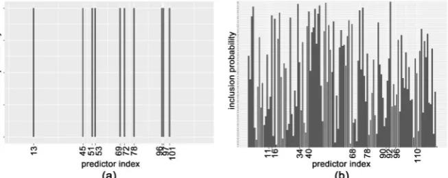
In this data, there are about 124 predictors, 5 non-predictors, and 18 response values. The details for each response value can be found at University of California, Irvine (UCI) Machine Learning Database [57]. Since this data has missing values and non-predictors, we preprocessed the data before applying our algorithm and BART on it. After the preprocessing, the number of observations n goes from 2215 to 114 observations, and the number of predictors p becomes 123. Therefore, in this example, we have a case that the number of predictors p is larger than the number of observation n. We split the data into 79 instances for training and 35 instances for testing. We investigated both algorithms’ performance in variable selection. We plotted the histogram of the Inclusion score for each variable in Figure 16.
Since BART and our algorithm has different Inclusion score values, we cannot pick the threshold values to identify variables for comparison. Since our algorithm only selects 10 predictors, we decided to rank predictors in BART based on their Inclusion score. Then, we chose BART’s top 10 predictors with highest Inclusion score to compare with ours. Table 7 lists selected factors affecting violent crime rate based on our algorithm and BART.
[image:18.595.213.540.561.691.2]According to Blumstein and Rosenfeld [58], the crime trend in the United States is contributed by the following factors 1) Economic condition 2) Policing 3) Control of firearms 4) Drugs markets 5) Gangs 6) Socialization and social service 7) Incarceration percent 8) Demographic change. Our selected variables can be grouped into three categories based on above factors. The first category
DOI: 10.4236/ojs.2017.74039 585 Open Journal of Statistics
Table 7. Selected variables between our algorithm and BART.
Variables Our Algorithm BART
1 % household with social security income % African-American
2 % Mom and kids under labor force income per capita for Asian heritage 3 % immigrants in the last 8 years % employed in manufacturing 4 % immigrants in the last 3 years % kids in two parents family 5 % housing occupied % of working mom 6 % vacant housing more than 6 months % kids in unmarried families 7 Number of housing occupied in upper quantile % immigrants in the last 8 years 8 Number of sworn full time police officer number of unit house built
9 Number of sworn police officer in operation number of housing without plumbing facilities 10 Total request for police per police officer % people living in the same city since 1985
is economic condition: variables 1, 2, 5, 6, and 7. The second category is demographic change: variables 3 and 4. The third category is policing: variables 8, 9, and 10. Similarly, selected variables in BART can be grouped into three categories. The first category is economic condition: variables 3, 2, 5 and 8. The second category is demographic change: variables 1 and 7. The third category is socialization and social service: variable 6. Based on these grouping, one can see that our selected variables is more agreeable to the study of Blumstein and Rosenfeld [58] than BART.
8. Conclusion
In this paper, we propose a novel Bayesian nonparametric approach for variable selection and interaction recovery with excellent performance in selection and interaction recovery in both simulated and real datasets. Our method obviates the computation bottleneck in recent unpublished work [28] by proposing a simpler regularization involving a combination of hard and soft shrinkage parameters.
Although such sparse additive models are well known to adapt to the underlying true dimension of the covariates [26], literature on consistent selection and interaction recovery in the context of nonparametric regression models is missing. As a future work, we propose to investigate consistency of the variable selection and interaction of our method.
References
[1] Manavalan, P. and Johnson, W.C. (1987) Variable Selection Method Improves the Prediction of Protein Secondary Structure from Circular Dichroism Spectra. Ana-lytical Biochemistry, 167, 76-85.
[2] Saeys, Y., Inza, I. and Larrañaga, P. (2007) A Review of Feature Selection Tech-niques in Bioinformatics. Bioinformatics, 23, 2507-2517.
DOI: 10.4236/ojs.2017.74039 586 Open Journal of Statistics Speech Signals. 8th European Conference on Speech Communication and Tech-nology, Geneva, 1-4 September 2003.
[4] Akaike, H. (1973) Maximum Likelihood Identification of Gaussian Autoregressive Moving Average Models. Biometrika, 60, 255-265.
https://doi.org/10.1093/biomet/60.2.255
[5] Schwarz, G., et al. (1978) Estimating the Dimension of a Model. The Annals of Sta-tistics, 6, 461-464.https://doi.org/10.1214/aos/1176344136
[6] Foster, D.P. and George, E.I. (1994) The Risk Ination Criterion for Multiple Regres-sion. The Annals of Statistics, 22, 1947-1975.
[7] Tibshirani, R. (1996) Regression Shrinkage and Selection via the Lasso. Journal of the Royal Statistical Society. Series B (Methodological), 58, 267-288.
[8] Efron, B., Hastie, T., Johnstone, I., Tibshirani, R., et al. (2004) Least Angle Regres-sion. The Annals of Statistics, 32, 407-499.
https://doi.org/10.1214/009053604000000067
[9] Fan, J. and Li, R. (2001) Variable Selection via Nonconcave Penalized Likelihood and Its Oracle Properties. JASA, 96, 1348-1360.
https://doi.org/10.1198/016214501753382273
[10] Zou, H. and Hastie, T. (2005) Regularization and Variable Selection via the Elastic Net. Journal of the Royal Statistical Society, Series B, 67, 301-320.
https://doi.org/10.1111/j.1467-9868.2005.00503.x
[11] Zou, H. (2006) The Adaptive Lasso and Its Oracle Properties. JASA, 101, 1418- 1429.https://doi.org/10.1198/016214506000000735
[12] Zhang, C.-H. (2010) Nearly Unbiased Variable Selection under Minimax Concave Penalty. The Annals of Statistics, 38, 894-942.https://doi.org/10.1214/09-AOS729 [13] Mitchell, T.J. and Beauchamp, J.J. (1988) Bayesian Variable Selection in Linear
Re-gression. JASA, 83, 1023-1032.https://doi.org/10.1080/01621459.1988.10478694 [14] George, E.I. and McCulloch, R.E. (1993) Variable Selection via Gibbs Sampling.
Journal of the American Statistical Association, 88, 881-889. https://doi.org/10.1080/01621459.1993.10476353
[15] George, E.I. and McCulloch, R.E. (1997) Approaches for Bayesian Variable Selec-tion. Statistica sinica, 7, 339-373.
[16] Laerty, J. and Wasserman, L. (2008) Rodeo: Sparse, Greedy Nonparametric Regres-sion. The Annals of Statistics, 36, 28-63.
[17] Wahba, G. (1990) Spline Models for Observational Data. Vol. 59, Siam. https://doi.org/10.1137/1.9781611970128
[18] Green, P.J. and Silverman, B.W. (1993) Nonparametric Regression and Generalized Linear Models: A Roughness Penalty Approach. CRC Press, Boca Raton.
[19] Hastie, T.J. and Tibshirani, R.J. (1990) Generalized Additive Models. Vol. 43, CRC Press, Boca Raton.
[20] Lin, Y., Zhang, H.H., et al. (2006) Component Selection and Smoothing in Multiva-riate Nonparametric Regression. The Annals of Statistics, 34, 2272-2297.
https://doi.org/10.1214/009053606000000722
[21] Ravikumar, P., Laerty, J., Liu, H. and Wasserman, L. (2009) Sparse Additive Models. Journal of the Royal Statistical Society: SeriesB (Statistical Methodology),71, 1009- 1030.https://doi.org/10.1111/j.1467-9868.2009.00718.x
DOI: 10.4236/ojs.2017.74039 587 Open Journal of Statistics Association, 105, 1541-1553.https://doi.org/10.1198/jasa.2010.tm10130
[23] Liu, D., Lin, X. and Ghosh, D. (2007) Semiparametric Regression of Multidimen-sional Genetic Pathway Data: Least-Squares Kernel Machines and Linear Mixed Models. Biometrics, 63, 1079-1088.
https://doi.org/10.1111/j.1541-0420.2007.00799.x
[24] Zou, F., Huang, H., Lee, S. and Hoeschele, I. (2010) Nonparametric Bayesian Varia-ble Selection with Applications to Multiple Quantitative Trait Loci Mapping with Epistasis and Gene-Environment Interaction. Genetics, 186, 385-394.
https://doi.org/10.1534/genetics.109.113688
[25] Savitsky, T., Vannucci, M. and Sha, N. (2011) Variable Selection for Nonparametric Gaussian Process Priors: Models and Computational Strategies. Statistical Science: A Review Journal of the Institute of Mathematical Statistics, 26, 130.
[26] Yang, Y., Tokdar, S.T., et al. (2015) Minimax-Optimal Nonparametric Regression in High Dimensions. The Annals of Statistics, 43, 652-674.
https://doi.org/10.1214/14-AOS1289
[27] Fang, Z., Kim, I. and Schaumont, P. (2012) Flexible Variable Selection for Recover-ing Sparsity in Nonadditive Nonparametric Models.
[28] Qamar, S. and Tokdar, S.T. (2014) Additive Gaussian Process Regression.
[29] Rasmussen, C.E. and Williams, C.K.I. (2006) Gaussian Processes for Machine Learning.
[30] Van der Vaart, A.W. and van Zanten, J.H. (2009) Adaptive Bayesian Estimation Using a Gaussian Random Field with Inverse Gamma Bandwidth. The Annals of Statistics, 37, 2655-2675.
[31] Bhattacharya, A., Pati, D. and Dunson, D.B. (2014) Anisotropic Function Estima-tion Using Multi-Bandwidth Gaussian Processes. The Annals of Statistics, 42, 352- 381.https://doi.org/10.1214/13-AOS1192
[32] Tibshirani, R., et al. (1997) The Lasso Method for Variable Selection in the Cox Model. Statistics in Medicine, 16, 385-395.
https://doi.org/10.1002/(SICI)1097-0258(19970228)16:4<385::AID-SIM380>3.0.CO; 2-3
[33] Hastie, T., Tibshirani, R., Friedman, J. and Franklin, J. (2005) The Elements of Sta-tistical Learning: Data Mining, Inference and Prediction. The Mathematical Intelli-gencer, 27, 83-85.https://doi.org/10.1007/BF02985802
[34] Park, T. and Casella, G. (2008) The Bayesian Lasso. Journal of the American Statis-tical Association, 103, 681-686.https://doi.org/10.1198/016214508000000337 [35] Tipping, M.E. (2001) Sparse Bayesian Learning and the Relevance Vector Machine.
The Journal of Machine Learning Research, 1, 211-244.
[36] Grin, J.E. and Brown, P.J. (2010) Inference with Normal-Gamma Prior Distribu-tions in Regression Problems. Bayesian Analysis, 5, 171-188.
https://doi.org/10.1214/10-BA507
[37] Carvalho, C.M., Polson, N.G. and Scott, J.G. (2010) The Horseshoe Estimator for Sparse Signals. Biometrika, 97, 465-480.https://doi.org/10.1093/biomet/asq017 [38] Carvalho, C.M., Polson, N.G. and Scott, J.G. (2009) Handling Sparsity via the
Horseshoe. International Conference on Artificial Intelligence and Statistics, Clearwater, 16-18 April 2009, 73-80.
DOI: 10.4236/ojs.2017.74039 588 Open Journal of Statistics [40] Polson, N.G. and Scott, J.G. (2010) Shrink Globally, Act Locally: Sparse Bayesian
Regularization and Prediction. Bayesian Statistics, 9, 501-538.
[41] Diebolt, J., Ip, E. and Olkin, I. (1994) A Stochastic EM Algorithm for Approximat-ing the Maximum Likelihood Estimate. Technical Report 301, Department of Statis-tics, Stanford University, Stanford.
[42] Meng, X.-L. and Rubin, D.B. (1994) On the Global and Component Wise Rates of Convergence of the EM Algorithm. Linear Algebra and Its Applications, 199, 413- 425.
[43] Hastings, W. (1970) Monte Carlo Sampling Methods Using Markov Chains and Their Applications. Biometrika, 57, 97-109.https://doi.org/10.1093/biomet/57.1.97 [44] Bishop, C.M. (2006) Pattern Recognition and Machine Learning. Springer, Berlin. [45] Han, J., Kamber, M. and Pei, J. (2011) Data Mining: Concepts and Techniques:
Concepts and Techniques. Elsevier, Amsterdam.
[46] Guyon, I. and Elisseeff, A. (2003) An Introduction to Variable and Feature Selec-tion. Journal of Machine Learning Research, 3, 1157-1182.
[47] George Forman (2003) An Extensive Empirical Study of Feature Selection Metrics for Text Classification. Journal of Machine Learning Research, 3, 1289-1305. [48] Stoppiglia, H., Dreyfus, G., Dubois, R. and Oussar, Y. (2003) Ranking a Random
Feature for Variable and Feature Selection. Journal of Machine Learning Research, 3, 1399-1414.
[49] Genuer, R., Poggi, J.M. and Tuleau-Malot, C. (2010) Variable Selection Using Ran-dom Forests. Pattern Recognition Letters, 31, 2225-2236.
[50] Chipman, H.A., George, E.I. and McCulloch, R.E. (2010) Bart: Bayesian Additive Regression Trees. The Annals of Applied Statistics, 4, 266-298.
[51] Harrison, D. and Rubinfeld, D.L. (1978) Hedonic Housing Prices and the Demand for Clean Air. Journal of Environmental Economics and Management, 5, 81-102. [52] Yeh, I., et al. (2008) Modeling Slump of Concrete with Yash and Superplasticizer.
Computers and Concrete, 5, 559-572.https://doi.org/10.12989/cac.2008.5.6.559 [53] Yeh, I.C. (2007) Modeling Slumpow of Concrete Using Second-Order Regressions
and Artificial Neural Networks. Cement and Concrete Composites, 29, 474-480. [54] Yurugi, M., Sakata, N., Iwai, M. and Sakai, G. (1993) Mix Proportion for Highly
Workable Concrete. Proceedings of Concrete, Dundee, 7-9 September 1993, 579- 589.
[55] Redmond, M.A. and Highley, T. (2010) Empirical Analysis of Caseediting Ap-proaches for Numeric Prediction. In: Innovations in Computing Sciences and Soft-ware Engineering,Springer, Berlin, 79-84.
[56] Buczak, A.L. and Gifford, C.M. (2010) Fuzzy Association Rule Mining for Commu-nity Crime Pattern Discovery. In: ACM SIGKDD Workshop on Intelligence and Security Informatics, ACM, New York, 2.
[57] Blake, C. and Merz, C.J. (1998) Repository of Machine Learning Databases.
Submit or recommend next manuscript to SCIRP and we will provide best service for you:
Accepting pre-submission inquiries through Email, Facebook, LinkedIn, Twitter, etc. A wide selection of journals (inclusive of 9 subjects, more than 200 journals)
Providing 24-hour high-quality service User-friendly online submission system Fair and swift peer-review system
Efficient typesetting and proofreading procedure
Display of the result of downloads and visits, as well as the number of cited articles Maximum dissemination of your research work