Munich Personal RePEc Archive
Decomposition of the Gender Wage Gap
in Indonesia: Analysis from Sakernas
Data
Weni Lidya, Sukma and Kadir, Kadir
Statistics Indonesia, Statistics Indonesia
3 February 2019
Online at
https://mpra.ub.uni-muenchen.de/94930/
Decomposition of the Gender Wage Gap in
Indonesia: Analysis from Sakernas Data
Weni Lidya Sukma Population and Labour Economics
University of Indonesia Jakarta, Indonesia weni.lidya@ui.ac.id
Kadir Applied Econometrics
Monash University Melbourne, Australia
Abstract—This paper investigates the gender wage gap in Indonesia by analyzing data from the 2016 Indonesia-National Labor Force Survey (SAKERNAS) to quantify the gap and decompose it into explained and unexplained gaps. Without controlling for differences in characteristics, we found that women were paid approximately 30 percent less than men. The results of the decomposition show that the explained gap accounts for only approximately one-fourth of the total gap. When casual workers in agricultural and non-agricultural are excluded from the analysis, women still earned 30 percent less than men, but the portion of the explained gap increases to just more than one-third of the total gap. The gender wage gap can be diminished through increases in women’s work hours, experience, education, and skills. Moreover, the high proportion of the unexplained gap indicates the presence of unfair discrimination against women. Therefore, reducing the level of gender discrimination in the labor market is also a critical factor in narrowing the gender wage gap in Indonesia.
Keywords—gender, SAKERNAS, decomposition, wage, discrimination
I. INTRODUCTION
Gender equality is an essential issue in Indonesia and one of the goals of national development. Unfortunately, although progress has been made and the capability gap between men and women has narrowed, the inequality between men and women still exists in many areas of life, including the job market.
The result of the National Labor Force Survey (SAKERNAS) indicated that the female labor force accounted for approximately 50 percent of the total labor force in August 2016. This fact explains the vital role that women play in contributing to the national economy through increases in household incomes that can ultimately be positive for enhancing economic growth.
Although women’s labor force participation rate reached 51 percent in August 2016 (BPS, 2016), the wage gap between males and females still exists across the employment sectors. In general, females earn lower wages than males. Predictably, the gap exists because of discrimination against women in the labor market and other factors, such as demographic conditions and differences in human capital and job characteristics between males and females.
This study aims to quantify the gender wage gap in Indonesia and examines some characteristics that can explain this gap by decomposing it into explained and unexplained parts. The explained part is considered to represent discrimination against women in the labor market, although this consideration raises debates among researchers.
A conventional technique often applied to decompose the gender wage gap is the Blinder-Oaxaca decomposition. This method enables the gap to be decomposed at the mean into explained and unexplained gaps. Studies that apply decomposition techniques in assessing the gender wage gap in Indonesia are still insufficient. Benjamin (1996) found that the unexplained part ranged from 62 to 81 percent after decomposing the gender wage gap among paid employees based on the survey year (1980 and 1990) and residential area (urban and rural). Meanwhile, using a sample limited to paid employees in an urban area with tertiary qualifications, Utomo (2008) found that the explained part accounted for 64 percent of the total gap.
To the best of our knowledge, Sohn (2015) conducted a recent study on the decomposition of the gender wage gap in Indonesia. That study used data from the Indonesian Family Life Survey undertaken in 2007 to decompose the gender wage gap in Indonesia for paid and unpaid employees. Additionally, decomposition was not only performed at the mean but also across the entire distribution. By excluding casual workers and the agricultural sector from the analysis, Sohn found that the explained gap comprised only approximately one-quarter of the total gap for paid employees and approximately one-half of the total gap for self-employees.
Our study is expected to enrich the literature on the decomposition of the gender wage gap in Indonesia by applying econometric techniques. The use of SAKERNAS data to analyze the gender wage gap in Indonesia is interesting and can be considered rare in the Indonesian case. Previously, Pirmana (2006) measured wage differentials between males and females in Indonesia using SAKERNAS data for the 1996, 1999, 2002, and 2004 survey periods. He found that, on average, the unexplained wage gap accounted for approximately 58 percent of the total gap during the period of study. Our research is expected to fill the gap in previous studies by enriching variables that can explain the variation in wages, comparing the results of various decomposition methods, and using more recent SAKERNAS data.
This study analyzes data from SAKERNAS, which was conducted by BPS-Statistics Indonesia in August 2016. The survey was started in 1986 and is conducted every year to capture employment conditions in Indonesia. By the year 2005, the survey had been carried out twice a year, in February and August. In August 2016, SAKERNAS covered 50,000 households scattered in urban and rural areas in 34 provinces. One of SAKERNAS’s advantages is the wealth of employment information possessed and its ability to present estimation results from national to provincial levels.
The labor theory approach used in SAKERNAS since 1984 is the Standard Labor Force Concept as outlined in the 13th International Conference of Labor Statistician (ICLS) 1982. In SAKERNAS, the working population is defined as the working-age population (15 years and older) conducting economic activities with the intention to obtain or assist in obtaining income or profits at least one hour (continuously) during the past week.
Given the limited information available, the work experience used in this research is potential work experience measured using the following approach: age minus years of schooling minus six years. Because information on years of schooling is not available, it is approached through highest educational attainment, which is converted into years of schooling.
The use of potential work experience potentially creates an upward bias in the measurement of work experience for women. This condition could arise because of the issue of career interruption that is common for women, mainly because of childbirth and child-rearing. For tenure, the potential bias is overcome by including its squared term.
Sample selection bias is one of the concerns in this study because wages are observed only for people who participate in the labor force (Jahn, 2008). Ideally, this selection bias is corrected by the inverse Mills Ratio proposed by Heckman (1976, 1979). However, given the limited information that explains labor force participation, we cannot apply this procedure, which means that the problem is not resolved.
This study focuses only on paid employees (wage earners), and the sample consists of 36,399 individuals. We exclude casual workers (7,525 observations) from the analysis because they have unique characteristics that are much different from those of laborers/employees.
The remainder of this paper is structured as follows. Section 2 highlights empirical studies that support the use of variables—especially the determinants of wage differentials—in this study. Furthermore, this section provides the framework of the analysis for constructing the model. Section 3 discusses the methodology, that is, the model specifications used and a brief explanation of the key variables included in the models. In section 4, we present a descriptive analysis and the estimation results of the models that focus on the key findings. Section 5 contains the conclusion of the study. Additional graphs and tables are presented in the Appendix.
II. ANALYTICALFRAMEWORK
Blau and Kahn (2003) proposed that one of the causes of gender wage differences is the demand and supply of female labor. The gap is indicated in the participation between men and women in the United States even after being controlled by education, experience, union engagement, jobs sector, and occupation. The results of their study show that education has a relatively positive influence on women’s wages relative to men’s wages.
Suh (2006) found changes in wage differences in the United States during 1998–2005. He pointed out that the gap narrowed significantly from 26 to 19 percent during the period of the study. He also controlled for marital status, occupation, and union engagement and found that an increase in women’s experience, working hours, and education can significantly narrow the gender wage gap.
Regarding Indonesia, Sohn (2015) analyzed the gender wage gap using the Indonesia Family Life Survey (ILFS) data collected in 2007. He found that the first quarter wage distribution was 30 percent lower for women than for men, and that the gap decreased in subsequent quarters. Variables used to explain the gap are, among others, marriage status, number of household members, number of children in a household, education, work experience, length of employment, employment contract, and residence.
Beheim, Himpele, Mahringer, and Zulehner (2010) studied the wage differential between males and females in Austria and found that females earned 12 percent less than males, and approximately 50 percent of the gap is unexplained. Their study used combined data on workers and employers for which the characteristics specified—education, experience, duration of employment, marital status, occupation, occupation, and type of enterprise— are consistent with those used in our paper.
The determinant of gender wage differences was illustrated in a study by Bowen et al. (2010). They sought to explain the potential factors that determined the gender wage gap across age groups and found that the greatest difference in wages between men and women occurred in the 45–54 year age range. The primary potential cause of this difference is education. In addition, other human capital variables are in the spotlight as significant factors.
The analytical framework used in our study to analyze the gender wage gap in Indonesia is presented in Figure 1. The main focus of our study is to gauge the impact of the gender variable on (log) wages. Thus, the average wage gap between males and females can be estimated. In addition, we also control for the impacts of other characteristics on wages, such as marital status, number of household members, number of household members younger than ten years, residence, education, experience, tenure, full-time employee, working hours, working contract, training, occupation, employment status, industry sector, and institution. We then decompose the total gap into the explained part, which is related to the differences in those characteristics between men and women, and the unexplained part. The high proportion of the unexplained part of the total gap can be
Fig. A1. Analytical framework of gender wage gap and its decomposition in Indonesia regression result
III. METHODOLOGY
To gauge the gender wage gap and analyze the characteristics that explain it, we develop an earning equation adopted from the well-known Mincer (1974) equation, with the following specification:
where denotes a monthly wage for individual i; is a vector of characteristics of the i-th individual; and is an i.i.d. error. However, this i.i.d. assumption for the error terms may be violated, particularly given the presence of heteroskedasticity as we work with high dimensional cross-sectional data. To overcome this issue, we correct the standard errors by clustering them at the subdistrict level (robust standard errors). Vector includes human capital variables, such as education, experience, the squared term of experience, tenure, and the squared term of tenure. In addition to the human capital variables that are the determinants of the wage level (Blau & Kahn, 2003), we also control for other variables in the analysis to overcome omitted variable bias, among others, variables representing demographic characteristics (marital status, number of household members, number of household members under ten years old) and job characteristics (average working hours per month, full-time employment, employment contract, union membership, participation in vocational training, overseas work experience, professional job, and blue-collar job). Taking into account the high segregation of gender by industry (Sohn, 2015) and institution in Indonesia, we also incorporate industrial and institutional dummy variables into the model specification. To control the specific effect of the province, such as the minimum regional wage and culture/social values, dummy variables that capture the provincial fixed effects are also included in the model. The definition and brief explanation of all variables included in the model specification are presented in Appendix Table A6.
The main focus of model (1) is to estimate , which captures the total gender gap in wages conditional to . In other words, shows the average wage differential between males and females by maintaining a constant . In equation (1), the reference group is male. Thus, the dummy variable is set to one if the individual is female and zero otherwise. The gender wage gap is quantified through the conversion of the log differentials formula ( )
Gender
Marital status Number of household
members
Number of household members under ten years old
Residence Education Expereience Tenure
Full-time employee Working hours Contract worker Training Occupation
Status of employment Fixed effect (Sector Industry,
Institution, Province)
Wages
Explained gap
Unexplained gap
Gender wage gap
Furthermore, the decomposition of the total gap is conducted by applying the method developed by Blinder (1973) and Oaxaca (1973). The decomposition is carried out by estimating the wage determination model individually for male (2) and female (3) using the ordinary least squares (OLS) method.
The total gap is decomposed into the explained and unexplained gaps using equation (4) by treating males as the reference group and using equation (5) by treating females as the reference group. Equation (4) corresponds to the “male-based” decomposition that assumes that males are paid their marginal product and females are negatively discriminated against. Meanwhile, equation (5) is a “female-based” view that assumes that women are paid their marginal product and men are positively discriminated against (Beheim, 2010).
̅̅̅̅̅̅̅ ̅̅̅̅̅̅̅ [ ̅̅̅̅̅̅ ̅̅̅̅̅] ̂ ̅̅̅̅̅̅[ ̂ ̂ ]
̅̅̅̅̅̅̅ ̅̅̅̅̅̅̅ [ ̅̅̅̅̅̅ ̅̅̅̅̅] ̂ ̅̅̅̅̅̅[ ̂ ̂ ]
The first term on the right-hand side of equations (4) and (5) explains how wage differences between men and women change in response to changes in the gap between male and female characteristics. This component is often called “observed gender gap in characteristics.” The second term on the right-hand side of equations (4) and (5) captures the unexplained portion of the wage gap concerning differences in coefficients or returns, which is considered to explain the level of gender discrimination.
The Blinder-Oaxaca decomposition is very sensitive to the determination of the reference group (Suh, 2006). In other words, decomposition by (4) and (5) will most likely produce different results. Equations (4) and (5) represent a specific form of the decomposition model proposed by Oaxaca and Ransom (1994), as follows:
̅̅̅̅̅̅̅ ̅̅̅̅̅̅̅ [ ̅̅̅̅̅̅ ̅̅̅̅̅] ̂ ̅̅̅̅̅̅[ ̂ ̂ ] ̅̅̅̅̅[ ̂ ̂ ]
where ̂ is the weighted average of the coefficient vectors ̂ and ̂ , which can be expressed as follows: ̂ ̂ ( ) ̂
where is the weighting matrix, and is the identity matrix. Equations (4) and (5) are special cases when is either a null matrix or an identity matrix. When is a null matrix, equation (6) obviously becomes equation (5). If is an identity matrix, equation (6) is identical to equation (4). Reimers (1983) assumed the same weighting for each coefficient, expressed as follows:
̂ ̂ ̂
whereas Cotton (1988) suggested weighting vectors coefficient with the proportions in two groups: ̂ ̂ ̂
In this study, we followed Oaxaca and Ransom (1994), who estimated a pooled model to derive the counterfactual coefficient vector. In comparison, the decomposition results derived using different techniques as proposed by Oaxaca and Ransom (1994), Reimers (1983), and Cotton (1988) are also presented.
As previously mentioned, the interpretation of the unexplained gap as earnings discrimination against females invites much debate. This interpretation can be explained because the unexplained part may arise not from gender discrimination but that the characteristics included in the analysis are insufficient. Therefore, interpreting this gap as evidence of gender discrimination may be an overstatement (Sohn, 2015). In this study, as a compromise from the debate, the unexplained gap is only interpreted as an “indication” of gender discrimination. To minimize the unobserved characteristics, we incorporate as many relevant characteristics as possible.
IV. RESULTS AND DISCUSSION A. Descriptive Analysis
the unexplained gap. For the laborer/employee group, the potential work experience of females is shorter by only 1.42 years relative to males, with the notion that this potential work experience may be biased upward because it does not consider the issue of females’ career interruption (motherhood and childcare responsibilities). Appendix Table A2 also confirms that casual workers have characteristics that are much different from those of laborers/employees. In general, casual workers are characterized by low human capital (education level), low-quality jobs, high concentrations in individual/household businesses, and sectors that rely on physical strength, such as agriculture and construction.
Regarding educational outcomes, females are much better than males, which are reflected in the larger proportion of females who have completed higher education (diploma and university) relative to males. Meanwhile, the percentage of married males is higher than for females. For the laborer/employee group, the proportion of married males reaches 69.12 percent, whereas the proportion of married women is 60.60 percent. This fact confirms the anecdotes that women tend to be dismissed from a job given marriage and childbirth and the tendency of companies to recruit unmarried women (ADB, 2006).
In the laborer/employee group, males are more likely to do menial jobs than females. In contrast to casual workers, the opportunity for females to engage in menial jobs is higher than that of males. Segregation between men and women is evident in some industries dominated by men, such as agriculture, mining and quarrying, construction and transportation, warehousing, and communications. For the laborer/employee group, we find that females are concentrated as office workers in government agencies (28.25 percent) and profit/private institutions (34.65 percent), whereas males are concentrated in individual/household businesses (40.99 percent ) and profit/private institutions (30.94 percent). According to the industry, both males and females are concentrated in the social service sector.
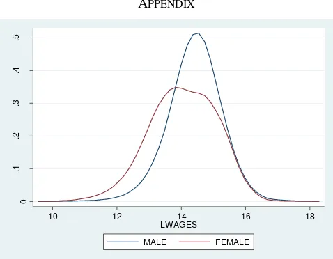
Appendix Figures A1 and A2 present the distribution of wages by gender for the entire sample (without excluding casual workers) and for the samples that exclude casual workers, respectively. For both cases, the density curve for a female is clearly located to the left of the density curve of the male. This finding indicates that, on average, women earn lower wages than men. Additionally, the variation in wage rates in females tends to be higher than for males.
B. Estimation Results of Earning Equation
Table 1 presents the estimation results of the earning equation for the pooled sample using OLS. Columns (1) and (3) display the estimation results for the entire sample and columns (2) and (4) present the estimation results without casual workers. When an only FEMALE variable is included in the model, as in column (1), women earn on average 30 percent less than men (( ) ). The wage difference is still the same without casual workers in the analysis, as shown in column (2). This finding is in line with those of Sohn (2015). Meanwhile, when the characteristics affecting wage rates are also controlled in the model, as in columns (3) and (4), the gender wage gap is reduced significantly to 23 percent for the entire sample, and approximately 20 percent of casual workers are excluded from the analysis. Again, these findings are in line with those of Sohn (2015).
In general, the estimation results indicate that the signs of all of the regression coefficients make sense and are consistent with the theory. The estimation results of the regression coefficients for all variables in the model with or without casual workers also do not show any significant differences. Additionally, all variables in the earnings equation together account for approximately 50 percent of the variation in the wage rate. This relatively high coefficient of determination is consistent with the statistical tests (see Appendix) that show that no variables were omitted in the model. In other words, all relevant variables to explain the wage variation have been included in the model. Thus, the estimates of the regression coefficients have a causal interpretation. Therefore, that all characteristics included in the model (including dummy variables for institution and industry) do not reduce the gender wage gap significantly is a strong indication of discrimination against women in earnings.
The estimates in columns (3) and (4) show that married workers on average earn approximately 5 percent higher wages (using the conversion formula) than unmarried workers. These results confirm the concept of the marriage premium in labor economics and the positive impact of educational attainment on wages, for which a higher education results in a higher wage earned by a worker. In line with Mincer (1974), work experience and tenure both significantly influence the wage level. Both show a normal U-shaped relationship with wage. Moreover, those who work as professionals receive higher wages than non-professionals. In general, a high-quality job characterized by a full-time job, working under a contract, and affiliation with a labor union earns a higher wage than a low-quality job. Job training also has a positive and significant impact on wage increase when, on average, workers attending vocational training earn an approximate 18 percent higher wage than workers who are not trained.
OLS ESTIMATION RESULTS OF EARNING EQUATION (POOLED SAMPLE)
(1) (2) (3) (4)
Female -0.357
(0.011)***
-0.349 (0.013)***
-0.264 (0.008)***
-0.222 (0.009)***
Married 0.066
(0.013)*** (0.014)0.069 ***
Number of household members -0.004
(0.003)
-0.005 (0.004)
Number of households members under ten years old 0.002
(0.008)
0.007 (0.009)
Urban 0.070
(0.011)*** (0.011)0.075 ***
Junior High School 0.127
(0.013)***
0.151 (0.014)***
Senior High School 0.250
(0.013)***
0.285 (0.015)***
Vocational High School 0.261
(0.013)*** (0.015)0.301 ***
Diploma 0.422
(0.027)***
0.452 (0.031)***
University 0.579
(0.022)***
0.604 (0.022)***
Work experience 0.011
(0.001)***
0.010 (0.002)***
Work experience squared/100 -0.017
(0.002)***
-0.014 (0.003)***
Tenure 0.025
(0.001)***
0.027 (0.002)***
Tenure squared/100 -0.030
(0.003)***
-0.020 (0.006)***
Overseas work experience 0.261
(0.050)***
0.320 (0.067)***
Full-time employee 0.424
(0.022)*** (0.024)0.474 ***
Working hours 0.002
(0.000)***
0.002 (0.000)***
Union member 0.208
(0.014)***
0.185 (0.014)***
Works under a contract 0.124
(0.012)*** (0.012)0.135 ***
Trained 0.200
(0.013)***
0.196 (0.013)***
Professional 0.097
(0.013)***
0.088 (0.013)***
Blue collar -0.052
(0.014)*** (0.016)-0.062 ***
Laborer/employee 0.096
(0.019)***
Constant 14.415
(0.018)***
14.547 (0.016)***
12.791 (0.050)***
12.891 (0.051)***
FE: industry, institution, and province Yes Yes
R2 0.039 0.039 0.514 0.497
Note: The entire sample consists of 36,339 observations (without casual workers: 28,814 observations). Sampling weights are applied. The reference group for school attainment is no school/primary school. Standard errors clustered at the subdistrict level are in parentheses. *p = 0.10; **p = 0.05; ***p = 0.01.
C. Decomposition Results
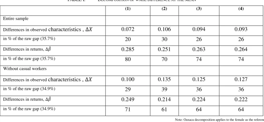
Table 2 presents the decomposition of the wage difference at the mean by including all of the characteristics used to estimate the earning equations in columns (3) and (4) in Table 1. Decomposition is performed for four different reference group methods, as previously discussed. In column (1), the reference group is female, indicating that female coefficients and male characteristics are used to estimate the counterfactual earnings of the female, as proposed by Oaxaca (1973). In column (2), male and female coefficients are equally weighted, as proposed by Reimers (1983). In column (3), the relative frequencies of the male and female groups are used as a weighting of the male and female coefficients, as proposed by Cotton (1988), whereas the estimated coefficients for column (4) with pooled samples are used to determine the counterfactual, as suggested by Oaxaca and Ransom (1994).
[image:8.595.67.529.81.592.2]As previously mentioned, our analysis focuses on the decomposition results based on the method proposed by Oaxaca and Ransom (1994) and presented in column (4) of Table 2. For the entire sample, the result of this technique indicates that the explained part covers only approximately 26 percent of the total gender wage gap. Without casual workers in the analysis, the share of the explained gap increases to approximately 36 percent. The high portion of the unexplained gap is a strong indication of discrimination against women in earnings. More details of the decomposition results presented in Appendix Tables A4 and A5 indicate that most of the explained part is attributed to the industry, which is the case because of the high segregation of gender according to the industry in Indonesia.
Decomposition results confirm the critical role of education in narrowing the gender wage gap. The negative sign of the explained part coefficient for educational characteristics indicates that the returns to education for females are higher than for males. Therefore, improving the level of education for females—mainly through higher education—can narrow the gap. As shown in Appendix Table A5, approximately –44 percent (–0.056/0.127 × 100%) of the explained gap is attributed to education. Therefore, on average, an increase in the level of education can reduce the gender wage gap by approximately 44 percent if casual workers are excluded from the analysis. In addition to education, improvements in job training and variables that are associated with a high-quality job (working under a contract, being a union member, and working as a professional) for women can also reduce the gap. Similarly, the squared terms of potential work experience and tenure both contribute to closing the gap.
[image:9.595.68.529.317.530.2]Further analysis of Appendix Tables A4 and A5 show that working hours, full-time employment, tenure, and potential work experience contribute significantly to widening the gender wage gap. Without casual workers in the analysis, approximately 39 percent of the explained gap is attributed to full-time employment, approximately 24 percent to working hours, 22 percent to tenure, and approximately 12 percent to potential work experience. Similarly, an identical pattern is observed for the entire sample. The results suggest that the gender wage gap exists partly given the difference between males and females regarding human capital (work experience and tenure) and job characteristics (full-time employment and working hours).
TABLE I. DECOMPOSITION OF WAGE DIFFERENCE AT THE MEAN
(1) (2) (3) (4)
Entire sample
Differences in observed characteristics , 0.072 0.106 0.094 0.093
in % of the raw gap (35.7%) 20 30 26 26
Differences in returns, ̂ 0.285 0.251 0.263 0.264
in % of the raw gap (35.7%) 80 70 74 74
Without casual workers
Differences in observed characteristics , 0.100 0.135 0.125 0.127
in % of the raw gap (34.9%) 29 39 36 36
Differences in returns, ̂ 0.249 0.214 0.224 0.222
in % of the raw gap (34.9%) 71 61 64 64
Note: Oaxaca decomposition applies to the female as the reference group.
V. CONCLUSIONS
This study confirms the existence of the gender wage gap in Indonesia. Regardless of other characteristics that affect the wage level, the average wage gap between men and women is estimated at approximately 30 percent. When other characteristics are also controlled for, the gap is narrowed significantly to approximately 20 percent. Meanwhile, the decomposition results show that the explained gap covers only approximately 30 percent of the total gap. The large proportion of the unexplained gap is a strong indication of discrimination against women in earnings. Therefore, reducing the level of gender discrimination in the labor market is also a critical factor in narrowing the gender wage gap in Indonesia.
However, because this study focuses only on the decomposition at the mean, which may not be representative in depicting the wage difference for the entire distribution, the decomposition across the distribution is highly recommended for a subsequent study to obtain a more precious picture of the difference in wages between males and females. Moreover, this study confirms the critical role of improving education, job training, and working hours for females in closing the gender wage gap. Additionally, the gaps in human capital (especially experience) and job characteristics contributed significantly to widening the wage difference between men and women. Therefore, these issues must also be addressed to close the gender wage gap in Indonesia.
REFERENCES
ADB (Asian Development Bank). (2006). Country Gender Assessment: Indonesia. Manila: ADB.
Benjamin, D. (1996). Women and the Labour Market in Indonesia during the 1980s. In Women and Industrialization in Asia, edited by Susan Horton, 81-133. London: Routledge.
Böheim, R., Himpele, K., Mahringer, H., & Zulehner, C. (2010). Determinants of wage differences between men and women in Austria. Institute of Economic Research.
BPS-Statistics Indonesia. (2016). The Labor Force Situation in Indonesia: August 2016. Jakarta: BPS. Cotton, J. (1988). On the decomposition of wage differentials. Review of Economics and Statistics, 70, 236-243.
Francine, D. B., & Lawrence M K. (2013). Understanding international differences in the gender pay gap. Journal of Labor Economics, 21(1), 106244. Heckman, J. J. (1976). The common structure of statistical models of truncation, sample selection and limited dependent variables and a simple estimator for
such models. Annals of Econometrics and Social Measurement, 5, 475–492.
Heckman, J. J. (1979). Sample selection bias as a specification error. Econometrica 47, 153–161.
Jahn, B. (2008). The Blinder-Oaxaca decomposition for linear regression model. Stata Journal, 8(4), 453-479.
Kitae, S. (2015). Gender discrimination in earnings in Indonesia: A fuller picture. Bulletin of Indonesian Economic Studies,51(1), 95-121. Liu, A. Y. C. (2004). Gender wage gap in Vietnam: 1993 to 1998. Journal of Comparative Economics, 32, 586-596.
Meng, X. (1998). Male–female wage determination and gender wage discrimination in China’s rural industrial sector. Labour Economics, 5, 67-89. Menon, N., & Yana van der M. R. (2009). International trade and the gender wage gap: new evidence from India’s manufacturing sector. World
Development, 37, 965-981.
Neumark, D. (1988). Employers’ discriminatory behaviour and the estimation of wage discrimination. Journal of Human Resources, 23, 279-295.
Neuman, S., & R. L. Oaxaca. (2004). Wage decompositions with selectivity-corrected wage equations: A methodological note. Journal of Economic Inequality, 2, 3-10.
Oaxaca, R. (1973). Male-female wage differentials in urban labour markets. International Economic Review, 14, 693-709.
Oaxaca, R. L., & M. R. Ransom. (1994). On discrimination and the decomposition of wage differentials. Journal of Econometrics, 61, 5-21.
Pirmana, V. (2006). Earnings Differential Between Male-Female In Indonesia: Evidence From Sakernas Data. Working Paper in Economics and Development Studies No. 200608.
Reimers, C. W. (1983). Labor market discrimination against Hispanic and black men. Review of Economics and Statistics, 65, 570-579. Suh, J. (2006). Decomposition of the change in the gender wage gap. Research in Business and Economics Journal, 1(1).
Mincer, J. A. (1974). Schooling, Experience, and Earnings. Cambridge, MA: National Bureau of Economic Research.
Utomo, A. J. (2008). Women as secondary earners: The labour market and marriage expectations of educated youth in urban Indonesia. PhD diss., The Australian National University.F. Koessler and A. Lambert-Mogiliansky, “Committing to transparency to resist corruption,”Journal of Development Economics, 100, 117-126.
.
[image:10.595.178.417.379.565.2]APPENDIX
Fig. A1. Wage distribution by gender (entire sample)
0
.1
.2
.3
.4
.5
10 12 14 16 18 LWAGES
MALE FEMALE
0
.1
.2
.3
.4
.5
10 12 14 16 18 LWAGES
Fig. A2. Wage distribution by gender (without casual workers)
TABLE A1DISTRIBUTION OF PAID EMPLOYEE BY EMPLOYMENT STATUS (%)
Employment status Male Female
Laborer/employee 75.18 85.57
Casual workers in non-agriculture 9.39 9.52
Casual workers in agriculture 15.43 4.90
Number of observations 24,176 12,163
TABLE A2DISTRIBUTION OF PAID EMPLOYEE BY EMPLOYMENT STATUS (%)
Variable Laborer/employee Casual workers
Male Female Male Female
Continuous variable (mean [SD]) 9.52
Log of monthly wage 14.55
(0.75)
14.20 (0.94)
14.02 (0.64)
13.23 (0.71)
Number of household members 4.28
(1.70)
4.26 (1.72)
4.15 (1.61)
3.76 (1.70) Number of household members under 10 years old 0.74
(0.85)
0.66 (0.82)
0.69 (0.79)
0.55 (0.75)
Monthly workhours (hour) 186.82
(49.15)
169.07 (54.37)
176.16 (50.85)
136.66 (59.60)
Potential work experience (year) 20.95
(12.60)
19.53 (13.13)
26.00 (14.22)
32.51 (13.83)
Tenure (year) 7.89
(8.18)
6.84 (7.74)
9.32 (9.93)
11.01 (11.16)
Dummy variable (%)
Married 69.12 60.60 74.70 73.58
Not married 30.88 39.40 25.30 26.42
Full-time employee 90.26 78.78 79.91 49.77
Part-time employee 9.74 21.22 20.09 50.23
Trained worker 21.95 26.10 2.61 1.41
Untrained worker 78.05 73.90 97.39 98.59
Works under a contract 60.55 66.95 16.26 13.20
Works without a contract 39.45 33.05 83.74 86.80
Blue-collar worker 20.03 18.60 60.91 65.49
Not a blue-collar worker 79.97 81.40 39.09 34.51
Professional worker 20.09 30.85 0.19 0.01
Not a professional worker 79.91 69.15 99.81 99.99
Has experience working overseas 0.53 0.27 1.07 0.58
Does not have experience working overseas 99.47 99.73 98.93 99.42
Union member 20.83 25.62 0.68 0.13
Not a union member 79.17 74.38 99.32 99.87
Urban residence 68.20 71.85 42.13 57.87
Rural residence 31.80 28.15 38.26 61.74
No school/primary school 20.81 18.23 62.48 79.79
Junior high school 16.99 13.52 22.87 13.01
[image:11.595.91.501.208.765.2]Variable Laborer/employee Casual workers
Male Female Male Female
Vocational high school 17.69 13.41 5.26 1.82
Diploma 3.80 8.62 0.12 0.15
University 15.85 27.32 0.21 0.35
Government organization/institution 19.87 28.25 0.87 0.11
International organization/institution 0.25 0.32 0.10 -
Non-profit organization 1.31 2.87 0.46 0.25
Profit institution (state-owned company, private
company) 40.99 34.65 4.77 3.12
Cooperative 0.86 0.72 0.14 0.04
Individual/household enterprise 30.94 21.53 62.83 67.72
Household 4.11 9.76 28.75 27.98
Others 1.16 1.68 1.59 0.60
Unknown 0.51 0.22 0.50 0.17
Agricultural 8.94 3.65 37.83 65.87
Mining, quarrying 2.39 0.30 2.38 1.06
Manufacturing 20.71 21.40 3.59 11.52
Gas, electricity, and water 0.97 0.19 0.1 -
Construction 9.47 0.59 43.59 1.73
Wholesale, retail, restaurants, and hotels 15.44 17.54 2.48 3.58
Transportation, storage, and communications 7.10 1.58 4.69 0.24
Finance, insurance, real estate, and business services 6.95 5.33 0.60 0.22
Social services 28.03 49.43 4.73 15.78
Number of observations 18,367 10,447 5,809 1,716
Omitted Variable Test
Ramsey RESET test using powers of the fitted values of LWAGES Ho: model has no omitted variables
F(3, 36263) = 0.88 Prob > F = 0.4530
Ramsey RESET test using powers of the fitted values of LWAGES Ho: model has no omitted variables
F(3, 28739) = 0.60 Prob > F = 0.6152
TABLE A3OLS ESTIMATION RESULTS OF EARNING EQUATION BY GENDER GROUP
Whole sample Without casual workers
Male Female Male Female
Married 0.132
(0.018)*** (0.017)0.019 (0.020)0.133 *** (0.019)0.033 *
Number of household members -0.007
(0.003)
-0.002 (0.006)
-0.008 (0.003)**
-0.002 (0.006) Number of households members under ten years old -0.002
(0.009)
-0.000 (0.010)
0.003 (0.011)
0.001 (0.011)
Urban 0.057
(0.011)*** (0.019)0.105 *** (0.012)0.061 *** (0.020)0.104 ***
Junior high school 0.091
(0.013)***
0.224 (0.026)***
0.114 (0.014)***
Whole sample Without casual workers
Male Female Male Female
Senior high school 0.204
(0.009)*** 0.409 (0.035)*** 0.238 (0.011)*** 0.420 (0.038)***
Vocational high school 0.216
(0.013)*** 0.413 (0.035)*** 0.257 (0.015)*** 0.424 (0.039)***
Diploma 0.349
(0.033)*** (0.044)0.589 *** (0.035)0.383 *** (0.047)0.602 ***
University 0.533
(0.023)*** 0.688 (0.039)*** 0.556 (0.024)*** 0.717 (0.041)***
Work experience 0.013
(0.001)*** (0.002)0.012 *** (0.002)0.013 *** (0.003)0.007 ***
Work experience squared/100 -0.022
(0.003)*** -0.013 (0.004)*** -0.021 (0.004)*** -0.004 (0.006)***
Tenure 0.021
(0.002)*** 0.033 (0.003)*** 0.022 (0.002)*** 0.035 (0.005)***
Tenure squared/100 -0.025
(0.004)*** -0.040 (0.008)*** -0.016 (0.006)*** -0.029 (0.015)**
Work experience abroad 0.264
(0.059)*** 0.234 (0.112)** 0.333 (0.083)*** 0.259 (0.127)**
Full-time employee 0.389
(0.023)*** 0.389 (0.030)*** 0.421 (0.026)*** 0.443 (0.033)***
Working hours 0.002
(0.000)*** (0.000)0.003 *** (0.000)0.001 *** (0.000)0.003 ***
Union member 0.136
(0.015)*** 0.303 (0.021)*** 0.116 (0.016)*** 0.276 (0.022)***
Works under contract 0.110
(0.014)*** 0.137 (0.018)*** 0.121 (0.016)*** 0.149 (0.018)***
Trained 0.171
(0.014)*** (0.028)0.232 *** (0.014)0.170 *** (0.027)0.222 ***
Professional 0.202
(0.019)*** -0.051 (0.032) 0.186 (0.019)*** -0.047 (0.031)
Blue-collar -0.082
(0.014)*** 0.029 (0.026) -0.082 (0.018)*** -0.012 (0.033)
Laborer/employee 0.072
(0.016)*** (0.038)0.187 ***
Constant 12.972
(0.054)*** 12.122 (0.095)*** 13.066 (0.061)*** 12.334 (0.104)***
FE: Industry, institution and province Yes Yes Yes Yes
R2 0.474 0.559 0.458 0.537
Note: The entire sample consists of 24,176 males and 12,163 females (without casual workers: 18,367 males and 10,447 females). Sampling weights are applied. The reference group for school attainment is no school/primary school. Standard errors clustered at the subdistrict level are in parentheses. *p = 0.10; **p = 0.05; ***p = 0.01.
TABLE A4DECOMPOSITION OF GENDER WAGE GAP AT THE MEAN (WHOLE SAMPLE)
Oaxaca
(Male Coefficient) Reimers Cotton Pooled
Total gap 0.357 (0.012)***
Total explained gap 0.072
(0.007)*** 0.106 (0.011)*** 0.094 (0.009)*** 0.093 (0.008)***
Married 0.011
(0.002)*** 0.006 (0.001)*** 0.008 (0.001)*** 0.005 (0.001)***
Number of household members -0.000
(0.000) -0.000 (0.000) -0.000 (0.000) -0.000 (0.000) Number of household members under ten years old -0.000
(0.001) -0.000 (0.001) -0.000 (0.001) 0.000 (0.001)
Urban -0.003
(0.001)*** -0.004 (0.001)*** -0.004 (0.001)*** -0.004 (0.001)***
Education -0.058
(0.004)*** -0.062 (0.004)*** -0.060 (0.003)*** -0.061 (0.003)***
Work experience 0.010
(0.003)*** (0.003)0.010 *** (0.003)0.010 *** (0.002)0.009 ***
Work experience squared/100 -0.003
(0.002) -0.002 (0.002) -0.002 (0.002) -0.002 (0.002)
Tenure 0.017
(0.003)*** 0.022 (0.004)*** 0.020 (0.004)*** 0.020 (0.004)***
Tenure squared/100 -0.004
(0.001)*** (0.002)-0.005 *** (0.002)-0.005 *** (0.002)-0.005 ***
Overseas work experience 0.001
(0.000)*** 0.001 (0.000)*** 0.001 (0.000)*** 0.001 (0.000)***
Oaxaca
(Male Coefficient) Reimers Cotton Pooled (0.003)*** (0.003)*** (0.003)*** (0.003)***
Working hours 0.032
(0.003)*** 0.045 (0.003)*** 0.040 (0.003)*** 0.041 (0.003)***
Union member -0.008
(0.001)*** -0.013 (0.001)*** -0.012 (0.001)*** -0.013 (0.001)***
Works under contract -0.011
(0.002)*** -0.012 (0.001)*** -0.011 (0.001)*** -0.012 (0.001)***
Trained -0.009
(0.001)*** -0.011 (0.001)*** -0.010 (0.001)*** -0.011 (0.001)***
Professional -0.023
(0.002)*** -0.008 (0.002)*** -0.012 (0.002)*** -0.011 (0.002)***
Blue-collar -0.004
(0.001)*** (0.001)-0.001 *** (0.001)-0.002 *** (0.001)-0.003 ***
Laborer/employee -0.008
(0.002)*** -0.013 (0.003)*** -0.011 (0.002)*** -0.010 (0.002)***
Institution 0.003
(0.003) -0.003 (0.003) -0.001 (0.003) 0.000 (0.003)
Industry 0.072
(0.005)*** (0.007)0.102 *** (0.006)0.092 *** (0.004)0.086 ***
Region 0.006
(0.003)** 0.007 (0.003)** 0.006 (0.003)** 0.007 (0.003)**
Total unexplained gap 0.285
(0.010)*** 0.251 (0.009)*** 0.263 (0.009)*** 0.264 (0.009)***
Note: The entire sample consists of 36,339 observations (without casual workers: 28,814 observations). Sampling weights are applied. Standard errors clustered at the subdistrict level are in parentheses. *p = 0.10; **p = 0.05; ***p = 0.01.
TABLE A5DECOMPOSITION OF GENDER WAGE GAP AT THE MEAN (WITHOUT CASUAL WORKERS)
Oaxaca
(Male Coefficient) Reimers Cotton Pooled
Total gap 0.349
(0.014)***
Total explained gap 0.100
(0.008)*** (0.011)0.135 *** (0.010)0.125 *** (0.009)0.127 ***
Married 0.011
(0.002)*** 0.007 (0.001)*** 0.008 (0.001)*** 0.006 (0.001)***
Number of household members -0.000
(0.000) -0.000 (0.000) -0.000 (0.000) -0.000 (0.000) Number of household members under ten years old 0.000
(0.001) 0.000 (0.001) 0.000 (0.001) 0.001 (0.001)
Urban -0.002
(0.001)*** -0.003 (0.001)*** -0.003 (0.001)*** -0.003 (0.001)***
Education -0.053
(0.003)*** -0.057 (0.003)*** -0.056 (0.003)*** -0.056 (0.003)***
Work experience 0.018
(0.004)*** 0.014 (0.003)*** 0.015 (0.003)*** 0.014 (0.003)***
Work experience squared/100 -0.009
(0.003) -0.005 (0.002) -0.006 (0.002) -0.006 (0.002)
Tenure 0.023
(0.003)*** 0.030 (0.004)*** 0.028 (0.004)*** 0.028 (0.004)***
Tenure squared/100 -0.004
(0.001)*** (0.002)-0.005 *** (0.002)-0.005 *** (0.001)-0.005 ***
Overseas work experience 0.001
(0.000)** 0.001 (0.000)** 0.001 (0.000)** 0.001 (0.000)**
Full-time employee 0.048
(0.004)*** 0.050 (0.003)*** 0.049 (0.003)*** 0.054 (0.003)***
Working hours 0.021
(0.003)*** (0.003)0.033 *** (0.003)0.030 *** (0.003)0.030 ***
Union member -0.006
(0.001)*** -0.009 (0.001)*** -0.008 (0.001)*** -0.009 (0.001)***
Works under contract -0.008
(0.001)*** -0.009 (0.001)*** -0.008 (0.001)*** -0.009 (0.001)***
Trained -0.007
(0.001)*** (0.001)-0.008 *** (0.001)-0.008 *** (0.001)-0.008 ***
Professional -0.020
(0.002)*** -0.008 (0.002)*** -0.011 (0.002)*** -0.009 (0.001)***
Blue-collar -0.001
(0.000)** -0.001 (0.000)* -0.001 (0.000)** -0.001 (0.000)**
Laborer/employee 0.014
(0.004)*** 0.007 (0.003)** 0.009 (0.003)*** 0.010 (0.003)***
Institution 0.060
Oaxaca
(Male Coefficient) Reimers Cotton Pooled
Industry 0.013
(0.003)*** (0.004)0.015 *** (0.004)0.015 *** (0.004)0.015 ***
Region 0.249
(0.012)***
0.214 (0.010)***
0.224 (0.010)***
0.222 (0.010)***
Total unexplained gap 0.285
(0.010)***
0.251 (0.009)***
0.263 (0.009)***
0.264 (0.009)***
Note: The entire sample consists of 36,339 observations (without casual workers: 28,814 observations). Standard errors clustered at subdistrict level are in parentheses. *p = 0.10; **p = 0.05; ***p = 0.01.
TABLE A6DEFINITIONS OF DEPENDENT AND EXPLANATORY VARIABLES
Dependent variable: logarithmic of monthly (nominal) wages.
Educational attainment University 1 if the highest qualification is university (bachelor degree, master degree, and PhD) and 0 otherwise; Diploma 1 if the highest qualification is Diploma I, II, or III and 0 otherwise;
Senior High School 1 if the highest qualification is senior high school and 0 otherwise; Vocational High School 1 if the highest qualification is vocational high school and 0 otherwise; Junior High School 1 if the highest qualification is junior high school and 0 otherwise; No School/Primary School 1 if the highest qualification is either no school completed or primary school and 0 otherwise (reference group).
Experience Experience is potential experience in years calculated by the formula: age minus years of schooling minus six years. Years of schooling is approached with the highest educational attainment converted into years of schooling.
Experience2 The squared of potential experience divided by 100.
Tenure Tenure is measured in years.
Tenure2 The squared of tenure divided by 100.
Demographic variables Female 1 if an individual is female and 0 otherwise; Married 1 if the marital status is married and 0 otherwise; Urban 1 if an individual lives in an urban area and 0 otherwise. Number of household members consists of two variables: the total number of household members and the number of household members under 10 years of age.
Working hours Working hours in a month (obtained by multiplying regular working hours of the week by four).
Job training Training 1 if an individual has been trained before and 0 otherwise.
Union membership Union 1 if an individual is the member of a labor union and 0 otherwise.
Employment status related to working hours Full employment 1 if an individual has full employment and 0 otherwise.
Occupation Professional 1 if the occupation is manager, professional, technicians, or police/army and 0 otherwise; Hard work 1 if the occupation is engaged in hard work (blue-collar) and 0 otherwise. Working under contract Contract 1 if an individual is working under a contract and 0
otherwise.
Dummy variables for Industries Employment sectors/industries consist of nine categories: agricultural (reference group); mining, quarrying; manufacturing; gas, electricity, and water; construction; wholesale, retail, restaurants and hotels; transportation, storage, and
communications; finance, insurance, real estate, and business services; social services.
Dummy variables for the institutions Employment institutions consist of eight categories: government (reference group); international institution/organization; non-profit institutions; profit institutions; cooperatives; individual/households business; households; others.