Granger causality in dynamic binary short panel data models

Munich Personal RePEc Archive

Granger causality in dynamic binary

short panel data models

Bartolucci, Francesco and Pigini, Claudia

University of Perugia, Marche Polytechnic University

13 March 2017

Online at

https://mpra.ub.uni-muenchen.de/77486/

Granger causality in dynamic binary

short panel data models

Francesco Bartolucci

Universit`a di Perugia (IT) francesco.bartolucci@unipg.it

Claudia Pigini

Universit`a Politecnica delle Marche and MoFiR (IT)

c.pigini@univpm.it

March 13, 2017

Abstract

Strict exogeneity of covariates other than the lagged dependent variable, and conditional on unobserved heterogeneity, is often required for consistent estimation of binary panel data models. This assumption is likely to be violated in practice because of feedback effects from the past of the outcome variable on the present value of covariates and no general solution is yet available. In this paper, we pro-vide the conditions for a logit model formulation that takes into account feedback effects without specifying a joint parametric model for the outcome and predeter-mined explanatory variables. Our formulation is based on the equivalence between Granger’s definition of noncausality and a modification of the Sims’ strict exogene-ity assumption for nonlinear panel data models, introduced by Chamberlain (1982) and for which we provide a more general theorem. We further propose estimating the model parameters with a recent fixed-effects approach based on pseudo condi-tional inference, adapted to the present case, thereby taking care of the correlation between individual permanent unobserved heterogeneity and the model’s covariates as well. Our results hold for short panels with a large number of cross-section units, a case of great interest in microeconomic applications.

Keywords: fixed effects, noncausality, predetermined covariates, pseudo-conditional inference, strict exogeneity.

1

Introduction

There is an increasing number of empirical microeconomic applications that require the estimation of binary panel data models, which are typically dynamic so as to account for state dependence (Heckman, 1981).1

In these contexts, strict exogeneity of covariates other than the lagged dependent variable, conditional on unobserved heterogeneity, is required for consistent estimation of the regression and state dependence parameters, when the estimation relies on correlated random effects or on fixed effects which are eliminated when conditioning on suitable sufficient statistics for the individual unobserved heterogeneity. However, the assumption of strict exogeneity is likely to be violated in practice because there may be feedback effects from the past of the outcome variable on the present values of the covariates, namely the model covariates may be Granger-caused by the response variable Granger (1969). While in linear models the mainstream approach to overcome this problem is to consider instrumental variables (Anderson and Hsiao, 1981; Arellano and Bond, 1991; Arellano and Bover, 1995; Blundell and Bond, 1998), considerably fewer results are available for nonlinear binary panel data models with predetermined covariates. This is particularly true with short binary panel data and no general solution is yet available, despite the relevance of binary these type of data in microeconomic applications.

Honor´e and Lewbel (2002) propose a semiparametric estimator for the parameters of a binary choice model with predetermined covariates. However, they provide identification conditions when there is a further regressor that is continuous, strictly exogenous, and independent of the individual specific effects. These requirements are often difficult to be fulfilled in practice. Arellano and Carrasco (2003) develop a semiparametric strategy based on the Generalized Method of Moments (gmm) estimator involving the probability distribution of the predetermined covariates (sample cell frequencies for discrete covari-ates or nonparametric smoothed estimcovari-ates for continuous covaricovari-ates) that can, however, be difficult to employ when the set of relevant explanatory variables is large. A differ-ent approach is taken by Wooldridge (2000), who proposes to specify a joint model for the response variable and the predetermined covariates; the model parameters are esti-mated by a correlated random-effects approach (Mundlak, 1978; Chamberlain, 1984), to account for the dependence between strictly exogenous explanatory variables and individ-ual unobserved effects, combined with a preliminary version of the Wooldridge (2005)’s

1_{Estimators of dynamic discrete choice models are employed in studies related to labor market}

solution to the initial conditions problem. Although this is an intuitive strategy, it re-lies on distributional assumptions on the individual unobserved heterogeneity; moreover, it is computationally demanding when the number of predetermined covariates is large and it requires strict exogeneity of the covariates used for the parametric random-effects correction.

A strategy similar to that developed by Wooldridge (2000) is adopted by Mosconi and Seri (2006), who test for the presence of feedback effects in binary bivariate time-series by means of Maximum Likelihood (ml)-based test statistics. They build their estimation and testing proposals on the definition of Granger causality (Granger, 1969), which is typical of the time series literature, as adapted to the nonlinear panel data setting by Chamberlain (1982) and Florens and Mouchart (1982). While attractive, Mosconi and Seri’s approach does not account for individual time-invariant unobserved heterogeneity and is better suited for quite long panels, whereas applications, such as intertemporal choices related to the labor market, poverty traps, and persistence in unemployment, often rely on very short time-series and a large number of cross-section units resulting from rotated surveys. Furthermore, in the short panel data setting, dealing properly with time-invariant unobserved heterogeneity is crucial for the attainability of the estimation results, since individual-specific effects are often correlated with the covariates of interest. Moreover, the focus is often on properly detecting the causal effects of past events of the phenomenon of interest, namely the truestate dependence, as opposed to the persistence generated by permanent individual unobserved heterogeneity (Heckman, 1981).

In this paper, we propose a logit model formulation for dynamic binary fixedT-panel data model that takes into account general forms of feedback effects from the past of the outcome variable on the present value of the covariates. Our formulation presents three main advantages with respect to the available solutions. First, it does not require the specification of a joint parametric model for the outcome and predetermined explanatory variables. In fact, the starting point to build the proposed formulation is the definition of noncausality (Granger, 1969), the violation of which corresponds to the presence of feedback effects, as stated in terms of conditional independence by Chamberlain (1982) for nonlinear models. Translating the definition of noncausality to a parametric model requires, however, the specification of the conditional probability for the covariates (x). On the contrary, we follow Chamberlain (1982) and introduce an equivalent definition based on a modification of Sims (1972)’s strict exogeneity for nonlinear models, which only involves specifying the probability for the binary dependent variable at each time occasion (yt) conditional on past, present, and future values ofx, and for which we provide a more general theorem of equivalence to noncausality.

augment the linear index function with a linear combination of the leads of the predeter-mined covariates, along with the lags of the binary dependent variable. We analytically prove that this augmented linear index function corresponds to the logit for the joint distribution of yt and the future values of x, under the assumption that the distribution of the predetermined covariates belongs to the exponential family with dispersion param-eters (Barndorff-Nielsen, 1978) and that their conditional means depend on time-fixed effects. In the other cases, we anyway assume a linear approximation which proves to be effective in series of simulations while allowing us to maintain a simple approach.

Third, the logit formulation allows for a fixed-effects estimation approach based on sufficient statistics for the incidental parameters, thus avoiding parametric assumptions on the distribution of the individual unobserved heterogeneity. In particular, we propose estimating the model parameters by means of a Pseudo Conditional Maximum Likeli-hood (pcml) estimator recently put forward by Bartolucci and Nigro (2012), and here adapted to the proposed extended formulation. They approximate the dynamic logit with a Quadratic Exponential (qe) model (Cox, 1972; Bartolucci and Nigro, 2010), which ad-mits a sufficient statistics for the incidental parameters and has the same interpretation as the dynamic logit model in terms of log-odds ratio between pairs of consecutive out-comes. In simpler contexts, this approach leads to a consistent estimator of the model parameters under the null hypothesis of absence of true state dependence, whereas has a reduced bias even with strong state dependence.

We study the finite sample properties of the pcml estimator for the proposed model through an extensive simulation study. The results show that thepcmlestimator exhibits a negligible bias, for both the regression parameter associated with the predetermined co-variate and the state dependence parameter, in the presence of substantial departures from noncausality. In addition, the estimation bias is almost negligible when the density of the predetermined covariate does not belong to the exponential family or its condi-tional mean depends on time-varying effects. It is also worth noting that the qualities of the proposed approach emerge for quite short T and a large number of cross-section units. Finally, the pcml is compared with the correlated random-effects mlestimator of Wooldridge (2005), adapted for the proposed formulation. Thismlestimator is consistent for the parameters of interest in presence of feedbacks, although remarkably less efficient than the pcml in estimating the state dependence parameter, especially with short T. However, differently from our approach, consistency relies on the assumption of indepen-dence between the predetermined covariates and the individual unobserved effects, which is hardly tenable in practice.

5 outlines the simulation study, and Section 6 provides main conclusions.

2

Definitions

Consider panel data for a sample ofn units observed atT occasions according to a single explanatory variable xit and binary response yit, with i = 1, . . . , n and t = 1, . . . , T, where the response variable is affected by a time-constant unobservable intercept ci. Also let xi,t1:t2 = (xit1, . . . , xit2)

′ _{and y}

i,t1:t2 = (yit1, . . . , yit2)

′ _{denote the column vectors with}

elements referred to the period from the t1-th to the t2-th occasion, so that xi = xi,1:T

and y_i =y_i,1:T are referred to the entire period of observation for the same sample unit i. Note that here we consider only one covariate to maintain the illustration simple, but all definitions and results below naturally extend to the case of more covariates per time occasion.

In this framework, and as illustrated in Chamberlain (1982), assuming that the eco-nomic life of any individual begins at time t= 1, the Granger’s definition of noncausality is:

Definition. g - The response (y) does not cause the covariate (x) conditional on the time-fixed effect (c) if xi,t+1 is conditionally independent of y_i,1:t, given ci and xi,1:t, for

all i and t, that is:

p(xi,t+1|ci,xi,1:t,y_i,1:t) =p(xi,t+1|ci,xi,1:t), i= 1, . . . , n, t= 1, . . . , T −1. (1)

Testing for g requires the knowledge and formulation of the model for each time-specific covariate given the the previous covariates and responses. However, following Chamberlain (1982), we introduce a condition that is the basis of the approach that we present in the next sections.

Definition. s’ - x is strictly exogenous with respect to y, given c and the past responses, if yit is independent of xi,t+1:T conditional onci, xi,1:t, and yi,1:_t−1, for all i and t, that is p(yit_|ci,xi,y_i,1:t−1) =p(yit|ci,xi,1:t,y_i,1:t−1), i= 1, . . . , n, t= 1, . . . , T −1, (2)

where y_i,t−1 disappears from the conditioning argument for t = 1.

The following result holds, whose proof is related to that provided in Chamberlain (1982).

Theorem 1. g and s’ are equivalent conditions.

Proof. g may be reformulated as

p(xi,t+1, ci,xi,1:t,y_i,1:t) p(ci,xi,1:t,y_i,1:t)

= p(xi,t+1, ci,xi,1:t)

p(ci,xi,1:t)

for all i. Exchanging the denominator at lhs with the numerator at rhs, the previous equality becomes

p(y_i,1:t|ci,xi,1:t+1) =p(y_i,1:t|ci,xi,1:t), t= 1, . . . , T −1,

which, by marginalization, implies that

p(y_i,1:s|ci,xi,1:t+1) =p(y_i,1:s|ci,xi,1:t), t = 1, . . . , T −1, s= 1, . . . , t.

Therefore, we have

p(yis_|ci,xi,1:t+1,yi,1:s−1) =p(yis|ci,xi,1:t,y_i,1:s−1), t= 1, . . . , T −1, s= 1, . . . , t.

Finally, by recursively using the previous expression for a fixed s and for t fromT ₋1 to

s we obtain condition s’ as defined in (2). Similarly,s’ implies that

p(xi,t+1:T|ci,xi,1:t,yi,1:t) =p(xi,t+1:T|ci,xi,1:t,yi,1:t−1), t= 1, . . . , T −1,

for all i and implies

p(xi,s+1|ci,xi,1:s,y_i,1:t) = p(xi,s+1|ci,xi,1:s,y_i,1:t−1), t = 1, . . . , T −1, s= 1, . . . , T −1,

which, in turn, leads to condition (1) and then g. ✷

It is worth noting that, apart from the case T = 2, definition s’ is stronger than the definition of strict exogeneity of Sims (1972) adapted to the case of binary panel data, which we denote by s. Then, being equivalent to s’, g implies s, but in general s does not imply g. In fact, s is expressed avoiding to condition on the previous responses:

Definition. s - x is strictly exogenous with respect to y, given c, if yit is independent of

xi,t+1:T conditional on ci and xi,1:t, for alli and t, that is

p(yit_|ci,xi) =p(yit|ci,xi,1:t), i= 1, . . . , n, t= 2, . . . , T. (3)

Theorem 2. g implies s.

Proof. Proceeding as in the proof of Theorem 1, g implies that

p(yis_|ci,xi,1:t+1) =p(yis|ci,xi,1:t), t= 1, . . . , T −1, s= 1, . . . , t.

Although the focus here is on nonlinear binary panel data models, it is useful to accompany the discussion with the Granger’s and the Sims’ definitions in the simpler context of linear models, as laid out by Chamberlain (1984), where testable restrictions on the regression parameters can be derived directly. The starting point is a linear panel data model of the form

yit=xitβ+ci+εit, i= 1, . . . , n, t= 1, . . . , T, (4)

where now the dependent variables yit are continuous and the error termsεit are iid. The usual exogeneity assumption is stated as

E(εit_|ci,xi) = 0, i= 1, . . . , n, t= 1, . . . , T, (5)

which rules out the lagged response variables from the regression specification, as well as possible feedback effects from past values of yit on to the present and future values of the covariate.

Now consider the minimum mean-square error linear predictor, denoted by E∗_{(·), and}

consider the following definitions, which hold for all i:

E∗(ci_|xi) = η+x′iλ, (6)

E∗(yit_|xi) = αt+x′iπt, t= 1, . . . , T, (7)

where λ = (λ1, . . . , λT)′ _{and π}

t = (πt1, . . . , πtT)′ are vectors of regression coefficients.

Equation (7) may also be expressed as

E∗(yi|xi) =α+Πxi,

withα= (α1, . . . , αT)′_{andΠ= (π1, . . . ,π}

T)′. It may be simply proved that assumptions

(4), (5), together with definition (6), imply that

Π=βI+1λ′,

where I is an identity matrix and 1 is a column vector of ones of suitable dimension; in the present case they are of dimension T. In Chamberlain (1984), the structure of Π is related to the definition of strict exogeneity in Sims (1972) for linear models (equiva-lent to condition s for binary models defined above) that, conditional on the permanent unobserved heterogeneity, is stated as

E∗(yit_|ci,xi) = E∗(yit|ci,xi,1:t), t = 1, . . . , T. (8)

(1969). In matrix notation, condition (8) can be written as

E∗(y_i|ci,xi) = ϕ+Ψxi+ciτ, (9)

where Ψ is a lower triangular matrix,τ = (τ1, . . . , τT)′_{, and ϕ= (ϕ1, . . . , ϕT)}′_.

Assump-tions (6) and (9) then imply the following structure for Π: Π=B+δλ′,

where B is a lower triangular matrix and δ = (δ1, . . . , δT)′_.

It is straightforward to translate the restrictions in the structure of Π to the linear index function of a nonlinear model. In fact, Chamberlain (1984) and then Wooldridge (2010, Section 15.8.2) show that a simple test for strict exogeneity,s, in binary panel data models can be readily derived by addingxi,t+1 to the set of explanatory variables. In the

next section we show not only that noncausality s’ can be tested in a similar manner within a dynamic model formulation, but also that the linear index augmented with

xi,t+1 represents, under rather general conditions, the exact log-odds ratio for the joint

probability of yit and xi,t+1 when s’ is violated, thereby providing a model formulation

that accounts for feedback effects and whose parameters may be consistently estimated.

3

Model formulation

Consider the general case in which, for i= 1, . . . , n andt = 1, . . . , T, we observe a binary response variable yit and a vector of k covariates denoted by xit. Then, we extend the

previous notation by introducing Xi,t1:t2 = (xit1, . . . ,xit2), with Xi = Xi,1:T being the

matrix of the covariates for all time occasions. In order to illustrate the proposed model, we first recall the main assumptions of the dynamic logit model.

3.1

Dynamic logit model

A standard formulation of a dynamic binary choice model assumes that, for i= 1, . . . , n

and t = 1, . . . , T, the binary response yit has conditional distribution

p(yit_|ci,Xi,y_i,1:t−1) =p(yit|ci,xit, yi,t−1), (10)

corresponding to a first-order Markov model for yit with dependence only on the present values of the explanatory variables. The above conditioning set can be easily enlarged to include further lags of xit and yit.

ch. 7, for a review), that is,

p(yit_|ci,xit, yi,t−1) =

exp [yit(ci+x′_itβ+yi,t−1γ)]

1 + exp (ci+x′_itβ+yi,t−1γ), t = 2, . . . , T, (11) the conditional distribution of the overall vector of responses becomes:

p(y_i,2:T|ci,Xi, yi1) =

exp

yi+ci+PT

t=2

yit(x′_itβ+yit−1γ)

T

Q

t=2

[1 + exp (ci +x′

itβ+yi,t−1γ)]

, (12)

where β andγ are the parameters of interest for the covariates and the true state depen-dence (Heckman, 1981), respectively, yi+ =

PT

t=2yit is thetotal score and the

individual-specific intercepts ci are often considered as nuisance parameters; moreover, the initial observation yi1 is considered as given.

Expression (10) embeds assumption s’ by excluding leads of xit from the probability

conditioning set. It therefore rules out feedbacks from the response variable to future covariates, that is, the Granger causality. Noncausality is often a hardly tenable assump-tion, as when the covariates of interest depend on individual choices. If covariates are predetermined, as opposed to strictly exogenous, estimation of the model parameters of interest can be severely biased, when estimation is based on eliminating or approximating

ci with quantities depending on the entire observed history of covariates (Mundlak, 1978; Chamberlain, 1984; Wooldridge, 2005).

3.2

Proposed model

As stated at the end of Section 2, dealing with violations of condition s’, formulated as in (2), amounts to propose a generalization of the standard dynamic binary choice model based on assumption (10). In order to allow for such violations, we specify the probability of yit conditional on individual intercept now denoted by di, Xi, and yi,1:t−1 as

p(yit_|di,Xi,y_i,1:t−1) = p(yit|di,Xi,t:t+1, yi,t−1), (13)

retaining the assumption that previous covariates and responses before yi,t−1 do not affect yit. Note that, differently from (10), the conditioning set on the rhs includes the first-order leads of xit. Moreover, we use a different symbol for the unobserved individual intercept

rather obvious, it strongly complicates the following exposition.2

Following the discussion in Chamberlain (1984) and the suggestion in Wooldridge (2010, 15.8.2) on testing the strict exogeneity assumption, a test for noncausality can be derived by specifying the model as

p(yit_|di,Xi,t:t+1, yi,t−1) =g− 1

(di+x′_itβ+x′_i,t+1ν+yi,t−1γ), t = 2, . . . , T −1,

where g−1

(_·) is an inverse link function. It is worth noting that the null hypothesis

H0 : ν = 0 corresponds to condition s’, and then to Granger noncausality g. The identification of β and γ in presence of departures from noncausality requires further assumptions that lead to the formulation here proposed. In particular, we rely on the logit formulation

p(yit_|di,Xi,t:t+1, yi,t−1) =

exp

yit di+x′

itβ+x′i,t+1ν +yit−1γ

1 + exp di+x′

itβ+x′i,t+1ν +yi,t−1γ

. (14)

Under a particular, very relevant, case this formulation is justified according to the fol-lowing arguments.

First of all, denote the conditional density of the distribution of the covariate vector

xi,t+1 as

f(xi,t+1|ξ_i,Xi,1:t,y_i,1:t) =f(xi,t+1|ξ_i,xit, yit), t = 1, . . . , T −1, (15)

whereξ_iis a column vector of time-fixed effects and the presence of yit allows for feedback effects.3

Then the logit for the distribution yit conditional on ci, ξ_i, Xi,t:t+1, and yi,t−1 is

log p(yit= 1|ci,ξi,Xi,t:t+1, yi,t−1)

p(yit= 0_|ci,ξ_i,Xi,t:t+1, yi,t−1)

= logf(yit = 1,xi,t+1|ci,ξi,xi,t, yi,t−1)

f(yit = 0,xi,t+1|ci,ξ_i,xit, yi,t−1)

=

logp(yit= 1|ci,xit, yi,t−1)f(xi,t+1|ξi,xit, yit = 1)

p(yit= 0_|ci,xit, yi,t−1)f(xi,t+1|ξ_i,xit, yit = 0)

, (16)

where the presence of time-fixed effects in the conditioning sets foryitandxitis determined

by (13) and (15).4

Furthermore, we assume that the probability of yit conditional on ci,

xit,yi,t−1 has the dynamic logit formulation expressed in (11) so that the above expression

2

Chamberlain (1984) reports an empirical example where the linear index function of a logit model corresponds to the lhs of sin (3), where all the available lags and leads of xit are used. However, this specification is valid only whent= 1 is the beginning of the subject’s economic life. We do not make the same assumption here.

3_{In assumption (15) we maintain the same first-order dynamic as for (13). Nevertheless the}

assump-tions on the conditioning set on the right-hand-side can be relaxed to include more lags ofxitandyit.

4_{Notice that the extension of (13) to a number of leads 1}

< H ≤ T −3 requires to rewrite the conditional density of covariates asQH

becomes

log p(yit = 1|ci,ξi,Xi,t:t+1, yi,t−1)

p(yit = 0_|ci,ξ_i,Xi,t:t+1, yi,t−1)

=ci+x′_itβ+yi,t−1γ+ logf(xi,t+1|ξi,xit, yit = 1)

f(xi,t+1|ξ_i,xit, yit = 0) .

The main point now is how to deal with the components involving the ratio between the conditional density of xi,t+1 for yit = 0 and yit = 1. Suppose that the conditional

distribution of xi,t+1 belongs to the following exponential family:

f(xi,t+1|ξi,xit, yit =z) =

exp[x′

i,t+1(ξi+ηz)]h(xi,t+1;σ)

K(ξ_i+η_z;σ) , t = 1, . . . , T −1, z = 0,1, (17) where h(xi,t+1) is an arbitrary strictly positive function, possibly depending on suitable

dispersion parameters σ, and K(_·) is the normalizing constant. Note that this structure also covers the case of xi,t+1 depending on time-fixed effects through ξ_i. The following

result holds, the proof of which is trivial.

Theorem 3. Under assumptions (11) and (17), we have

logp(yit = 1|ci,ξi,Xi,t:t+1, yi,t−1) p(yit = 0_|ci,ξ_i,Xi,t:t+1, yi,t−1)

= logp(yit = 1|di,Xi,t:t+1, yi,t−1)

p(yit = 0_|di,Xi,t:t+1, yi,t−1)

=

di+x′_itβ+x′_i,t+1ν+yi,t−1γ,

where di = ci+ logK(ξ_i+η1;σ)−logK(ξi +η0;σ) and ν =η1−η0, and then model

(14) holds.

Two cases satisfying (17) are for continuous covariates having multivariate normal distribution with common variance-covariance matrix and the case of binary covariates. More precisely, in the first case suppose that

xi,t+1|ci,xit, yit=z ∼N(ζ_i+µ_z,Σ);

then (17) holds with ξ_i = Σ−1ζ_i and η_z = Σ−1µ_z, z = 0,1, where the upper (lower) triangular part of Σgo in ψ. Regarding the second case, we suppose that given ξ_i, Xit,

and yit =z, the elements of xi,t+1 are conditionally independent, with the j-th element

having Bernoulli distribution with success probability

exp(ξij+ηzj)

1 + exp(ξij +ηzj), j = 1, . . . , k,

where k is the number of covariates. In the other cases, when (17) does not hold, we anyway assume a linear approximation for the ratio between the conditional density of

xi,t+1 for yit = 0 and yit = 1 in (16) which is the most natural solution to maintain an

For the following developments, it is convenient to derive the conditional distribution of the entire vector of responses, which holds under the extended logit formulation (14) and that directly compares with (12). For all i, the distribution at issue is

p(y_i,2:T−1|di,Xi, yi1, yiT) = (18)

exp

y∗ i+di+

T−1

P

t=2

yit x′_itβ+x′_i,t+1ν +yit−1γ

T−1

Q

t=2

1 + exp di+x′_itβ+x′_i,t+1ν +yi,t−1γ

.

where y∗ i+ =

T−1

P

t=2

yit. In particular, model (18) reduces to the dynamic logit (12) under

the null hypothesis of noncausality H0 : ν = 0, if the probability in (12) is conditioned on yiT and with different individual intercepts.

The parameters in (18) can be estimated by either a random- or fixed-effects approach, keeping in mind that a (correlated) random-effects strategy (Mundlak, 1978; Chamber-lain, 1984) requires the predetermined covariates in xit to be independent of di. As this

assumption may often be hardly tenable, in the next section we discuss a fixed-effects estimation approach, first put forward by Bartolucci and Nigro (2012) and here adapted to the present case.

4

Fixed-effects estimation

4.1

Approximating model

The approximating model for (18) is derived by taking a linearization of the log-probability of the latter, similar to that used in Bartolucci and Nigro (2012), that is,

logp(y_i,2:T−1|di,Xi, yi1, yiT) = y ∗ i+di+

T−1

X

t=2

yit x′_itβ+x′_i,t+1ν +yi,t−1γ

−

T−1

X

t=2

log

1 + exp di+x′_itβ+x′_i,t+1ν+yi,t−1γ

. (19)

The term that is nonlinear in the parameters is approximated by a first-order Taylor series expansion around di = ¯di, β= ¯β,ν = ¯ν, and γ = 0, leading to

T−1

X

t=2

log

1 + exp di+x′_itβ¯+x′_i,t+1ν +yi,t−1γ

≈

T−1

X

t=2

1 + exp ¯di+x′_itβ¯ +x′_i,t+1ν¯

+

T−1

X

t=2 qit

di₋di¯ +x′_it β₋β¯

+x′_i,t+1(ν₋ν¯)

+

T−1

X

t=2

qityi,t−1γ, (20)

where

qit = exp ¯di +x

′

itβ¯ +x′i,t+1ν¯

1 + exp ¯di+x′

itβ¯+x′i,t+1ν¯

.

Since only the last sum in (20) depends on y_i,2:T−1, we can substitute (20) in (19) and

obtain the approximation of the joint probability (18) that gives the following qe model

p∗(y_i,2:T−1|di,Xi, yi1, yiT) =

exp

y∗ i+di+

T−1

P

t=2

yit x′_itβ+x′_i,t+1ν

+P

t

(yit₋qit)yi,t−1γ

P

z2:T₋1

exp

z∗_+di+T− 1

P

t=2 zt x′

itβ+x′i,t+1ν

+P

t

(zt₋qit)ztγ

, (21)

where the sum at the denominator ranges over all the possible binary response vectors

z2:T−1 = (z2, . . . , zT₋1)′ and z+∗ = T−1

P

t=2

zt, withz1 =yi1.

The joint probability in (21) is closely related to the probability of the response con-figuration y_i,2:T−1 in the true model in (18). In particular, the approximating qeand the

proposed true model share the properties summarized by the following theorem that can be proved along the lines of Bartolucci and Nigro (2010):5

Theorem 4. For i= 1, . . . , n:

(i) In the case of γ = 0, the joint probability p∗_(y

i,2:T−1|di,Xi, yi1, yiT) does not depend

onyi,t−1 or onqit, and both the true (18) and approximating model (21), correspond

to the following static logit model

p∗(y_i,2:T−1|di,Xi, yi1, yiT) =

exp

y∗ i+di+

T−1

P

t=2

yit x′_itβ+x′_i,t+1ν

P

z2:T₋1

exp

z_+di∗ _{+ x}′

itβ+x′i,t+1ν

=

T−1

Y

t=2

exp

yit di+x′_itβ+x′_i,t+1ν

1 + exp di +x′

itβ+x′i,t+1ν

.

(ii) yit is conditionally independent of y_i,1:t−2 given di, Xi, and yi,t−1, for t = 2, . . . , T.

(iii) Under both models, the parameterγ has the same interpretation in terms of log-odds ratio between the responses yit and yi,t−1, for t= 2, . . . , T −1:

logp

∗_{(yit= 1|di,Xi, yi,t−} 1 = 1) p∗_{(yit= 0|di,Xi, yi,t−1 = 1)} −log

p∗_{(yit= 1|di,Xi, yi,t−} 1 = 0) p∗_{(yit= 0|di,Xi, yi,t−1 = 0)} =γ.

The nice feature of the qe model in (21) is that it admits sufficient statistics for the incidental parameters di, which are the total scores y∗

i+ for i= 1, . . . , n. The probability

of y_i,2:T−1, conditional on Xi,yi1, yiT, and y_i∗+, for the approximating model is then

p∗ y_i,2:T−1|Xi, yi1, yiT, y ∗ i+

=

exp

_T−1

P

t=2 yit x′

itβ+x′i,t+1ν

+

T−1

P

t=2

(yit₋qit)yi,t−1γ

P

z2:T₋1

z∗

+=y∗i+

exp

_T−1

P

t=2 zt x′

itβ+x′i,t+1ν

+

T−1

P

t=2

(zt₋qit)zt−1γ

, (22)

which no longer depends on di and where the sum at the denominator is extended to all

the possible response configurations z2:T−1 such that z+∗ =yi∗+, wherez+∗ = T−1

P

t=2

.

4.2

Pseudo conditional maximum likelihood estimator

The formulation of the conditional log-likelihood for (22) relies on the fixed quantitiesqit, that are based on a preliminary estimation of the parameters associated with the covariate and of the individual effects. Let φ= (β′,ν′)′ _{be the vector collecting all the regression}

parameters and θ = (φ′,γ′)′_{. The estimation approach is based on two-steps:}

1. Preliminary estimates of the parameters needed to compute qit are obtained by maximizing the following conditional log-likelihood

ℓ( ¯φ) =

n

X

i=1

1_{0< yit < T ₋2_}ℓi( ¯φ),

ℓi( ¯φ) = log

exp

_T−1

P

t=2

yit x′_itβ¯+x′_i,t+1ν¯

P

z2:T₋1

z∗

+=yi∗+

exp

_T−1

P

t=2

zt x′_itβ¯ +x′_i,t+1ν¯

,

which can be maximized by a Newton-Raphson algorithm.

2. The parameter vector θ is estimated by maximizing the conditional log-likelihood of (22), that can be written as

ℓ∗(θ_|φ¯) = X

i

1_{0< yit <(T ₋2)_}ℓ∗_i(θ_|φ¯), (23)

ℓ_i∗(θ_|φ¯) = logp∗_θ|φ¯(y_i,2:T−1|Xi, yi1, yi1, y ∗ i+).

The resulting ˆθ is the pseudo conditional maximum likelihood estimator.

Functionℓ∗_(θ|φ¯_{) may be maximized by Newton-Raphson using the score and observed}

information matrix reported below (Section 4.2.1). We also illustrate how to derive stan-dard errors for the two-step estimator (Section 4.2.2). We leave out of the exposition the asymptotic properties of the pcml estimator, which can be derived along the same lines as in Bartolucci and Nigro (2012).

4.2.1 Score and information matrix

In order to write the score and information matrix forθ, it is convenient to rewriteℓ∗ i(θ|φ¯)

as

ℓ∗_i(θ_|φ¯) = u∗(y_i,1:T−1)

′_A∗_(X i)′θ−

log X z2:T₋1

z∗

+=y∗i+

exp [u∗(zi,1:T−1)′A∗(Xi)′θ], (24)

where the notation u∗(y_i,1:T−1) is used to stress that u∗ is a function of both the initial

and z2:T−1, since z1 =yi1 as in (21). Moreover u∗(y_i,1:T−1) and A ∗_(X

i) in (24) are

u∗(y_i,1:T−1) = y′i,2:T−1, T−1

X

t=2

(yit₋qit)yi,t−1

!′

A∗(Xi) =

Xi,2:T 0

0′ 1

, (25)

where Xi,2:T is a matrix of T −1 rows and 2k columns, withk the number of covariates

and typical row x′_i,t:t+1, while 0 is column vector of zeros having a suitable dimension. 6

Using the above notation, the score s∗(θ_|φ¯) = _∇θℓ∗i(θ|φ¯) and the observed information

matrix J∗(θ_|φ¯) =_−∇θθℓ∗i(θ|φ¯) are

s∗(θ_|φ¯) = X

i

1_{0< y_i∗+< T −2}A ∗_(X

i){u∗(yi,2:T−1)−

E∗_θ|φ¯

u∗(y_i,2:T−1)|Xi, yi1, , yiT, y ∗ i+

}, (26)

and

J∗(θ_|φ¯) = X

i

1_{0< y∗

i+ < T −2}A ∗_(X

i)×

V_θ∗_|φ¯

u∗(y_i,2:T−1)|Xi, yi1, y ∗ i+

A∗(Xi)′, (27)

where the conditional expected value and variance are defined as

E∗_θ|φ¯

u∗(y_i,2:T−1)|Xi, yi1, yi+∗

=

X

zH+1:T₋H

z∗

+=yi∗+

u∗(zi,2:T−2)p∗_θ|φ¯ zi,2:T−2|Xi, yi1, y_i∗+

,

and

V_θ∗_|φ¯

u∗(y_i,2:T−1)|Xi,yi,1:H, y ∗ i+

=

E∗_θ|φ¯

u∗(y_i,2:T−1)u∗(yi,2:T−1)′|Xi, yi1, y∗i+

−

E∗_θ|φ¯

u∗(y_i,2:T−1)|Xi, yi1, y ∗ i+

E∗_θ|φ¯

u∗(y_i,2:T−1)|Xi, yi1, y_i∗+

′

.

Following the results in Bartolucci and Nigro (2012), which can be applied directly to

6_{In order to clarify the structure of}

A∗_(X

i), consider the simple case ofT = 4 time occasions and one covariate. Then

A∗_(X

i) =

xi2 xi3 0

xi3 xi4 0

0 0 1

!

the present case,ℓ∗_{(θ|φ¯) is always concave andJ}∗_(θ

|φ¯) is almost surely positive definite.7

Then ˆθ that maximizesℓ∗_{(θ|φ¯) is found at convergence of the standard Newton-Raphson}

algorithm.

4.2.2 Standard errors

The computation of standard errors must take into account the first step estimation of ¯φ. As Bartolucci and Nigro (2012) we also rely on the gmm approach (Hansen, 1982) and cast the estimating equations as

m( ¯φ,θ) =

n

X

i=1

1_{0< y∗_i+ < T −2}mi( ¯φ,θ) = 0,

where mi( ¯φ,θ) contains the score vectors of the first step, ∇_φ¯ℓi( ¯φ), and of the second

step, _∇θ|_φ¯ℓ∗_i(θ|φ¯). Then thegmm estimator is ( ˜φ ′

,θˆ′)′ _{and its variance-covariance matrix}

can be estimated as

V( ˜φ,θˆ) = H( ˜φ,θˆ)−1

S( ˜φ,θˆ)hH( ˜φ,θˆ)−1i′ ,

where

S( ¯φ,θ) = X

i

1_{0< yi+∗ < T −2}mi( ¯φ,θ)mi( ¯φ,θ)′,

H( ¯φ,θ) = X

i

1_{0< y_i∗+ < T −2}Hi( ¯φ,θ).

Matrix Hi( ¯φ,θ) is composed of four blocks as follows:

Hi( ¯φ,θ) =

∇_φ¯_φ¯ℓi( ¯φ) 0

∇θφ¯ℓ∗i(θ|β¯) ∇θθℓ∗i(θ|β¯)

.

The north-west block is expressed as

∇_φ¯_φ¯ℓi( ¯φ) =X_i,2:TV_φ¯u(y_i,2:T−1)|Xi, yi1, yiT, y_i∗₊X′_i,2:T,

whereXi,2:T is defined in (25) and V_φ¯ is the conditional variance in the static logit model.

Moreover, _∇θθℓ∗i(θ|φ¯) is equal to −J ∗_(θ

|φ¯); see definition (27). Finally, the derivation of _∇θφ¯ℓ∗i(θ|φ¯) is not straightforward and we therefore rely on the numerical derivative of

(26) with respect to ¯φ.

5

Simulation study

In this section we describe the design and illustrate the main results of the simulation study we used to investigate about the final sample properties of the pcml estimator for the parameters of the proposed model formulation. In the first part of the study, the main focus is on the performance under substantial departures from noncausality, which we obtain by a non-zero effect from the past values of the binary dependent variable on the present value of the covariate. In the second part, we compare thepcml estimator of (18) with an alternative ml random-effects estimator for the same model, based on the proposal by Wooldridge (2005) to account for the initial condition problem.

5.1

Simulation design

The simulation study is based on samples drawn from a dynamic logit model, where the linear index specification includes the lagged dependent variable, one explanatory variable

xit possibly predetermined, one strictly exogenous variablevit, and individual unobserved heterogeneity. The model assumes that

yit = 1_{ci+βxit₋0.5vit+γyit−1+εit≥0}, (28)

for i= 1, . . . , n, t= 2, . . . , T, with initial condition

yi1 = 1{ci+βxi1−0.5vi1+εi1 ≥0}.

In the considered scenarios, the error terms εit, t= 1, . . . , T, follow a logistic distribution with zero mean and variance equal to π2

/3 and the individual specific intercepts ci are allowed to be correlated with xit and vit.

We consider a benchmark design and some extensions that are characterized by differ-ent choices for the distribution of the explanatory variable xit. The general formulation is

xit = w(ξi+x_it∗ +ψvit+ηyit−1), (29)

x∗it ∼ N(0, π 2

/3),

fort= 2, . . . , T, the initial value isxi1 =w(ξi+x∗_i1+ψvi1) withx∗_i1being again a zero mean

normal with variance π2

/3, andvit =ξi+v∗

it, fort= 1, . . . , T, wherev∗itis alsoN(0, π 2

hold and the model formulated in Theorem 3 is an approximation: first, we letw(_·) be an indicator function so thatxitbecomes a binary covariate with a normally distributed error term, withp(xit= 1_|ξi, vit, yi,t−1) = Φ(ξi+x∗_it+ψvit+ηyi,t−1), where Φ(·) is the standard

normal cdf and therefore does not belong to the exponential family in (17); secondly, we let the w(_·) be the identity function and setψ = 0.5 in order for xit to depend on other time varying covariates.

Based on x∗

it, the individual intercepts ci and ξi are derived as

ci = (1/T)

4

X

t=1

x∗_it, (30)

ξi = ̟ ci+√1₋̟2_uit,

with̟ = 0.5,uit _∼N(0,1) and fori= 1, . . . , n. This way, the generating model admits a correlation between the covariates and the individual-specific intercepts and dependence between the unobserved heterogeneity in both processes for y and x.

In most economic applications, the parameters of interest are γ, measuring the state dependence, and the regression coefficient β. Based on the generating model (28), we ran experiments for scenarios with γ = 0,1 and β = 0,₋1. We examine violations of noncausality by setting η = ₋1, compared with the same scenarios with η = 0. The chosen values for β, γ, and η are consistent with likely situations in practice that relate, for instance, to the feedback effect of past employment on present child birth when an-alyzing female labor supply (see also Mosconi and Seri, 2006, for a related application). Notice that here we are implicitly assuming that the only source of contemporaneous en-dogeneity, namely the reverse causality betweenxit andyit, is completely captured by the correlation between the individual specific intercepts in the two processes. The sample sizes considered are n = 500,1000 for T = 4,8. The number of Monte Carlo replications is 1000.

5.2

Main results

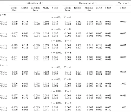
Tables 1–6 report the main results of our simulation study. Tables 1–4 show the results for the benchmark design, under which the covariate xit, generated as in (29), is normally distributed, with w(_·) being the identity function, and ψ = 0, for all the combinations of the chosen values of β and γ. Tables 5 and 6 report the simulation results for the two extensions of our benchmark design, under which xitis generated as a binary variable and with a dependence on the time varying covariate vit, respectively, for β=₋1,γ = 1, and

η = 0,₋1.

alternative hypotheses of noncausality described by s’ in Section 2: pcml1 denotes the

pcml estimator for the parameters in (18); pcml0 denotes the estimator of (18) with

the constraint ν = 0. For each estimator, we report the mean bias, the median bias, the root-mean square error (RMSE), the median absolute error (MAE), as in Honor´e and Kyriazidou (2000), and thet-tests at the 5% nominal size for H0 : ˆβ =β, andH0 : ˆγ =γ. Finally we report the t-tests at the 5% nominal size for noncausality, H0 : ν = 0. We expect pcml0 to yield biased estimators when η 6= 0 since, following s’, the lead of xit

is omitted from the model specification. We limit the discussion to the estimation of β

and γ, which are likely to be the parameters of main interest in applications. Results concerning the other model parameters are available upon request.

Table 1 summarizes the simulation results for our benchmark design and β =γ = 0. With η = 0, that is, in absence of feedback effects, the mean bias and median bias are always negligible, whereas the MAE and RMSE decrease with both n and T for the two models considered. While the same considerations hold forpcml1 whenη=−1, thepcml

estimators of β provided by pcml0 is severely biased and leads to misleading inference,

although this pattern is alleviated for T = 8. The same patterns are shown in Table 2, where β is equal to ₋1. Moreover, the t-test for H0 : ν = 0 always attains its nominal size and exhibits strong empirical power in all the scenarios with η=₋1

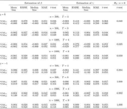
Tables 3 and 4 summarize simulation results for the same designs when γ = 1. They depict similar situations to those in Tables 1 and 2, with the exception of the bias of γ, that slightly increases. In fact, the performance of the pcmlestimator may be especially sensitive to the degree of state dependence in the generated samples. A high value of

γ leads to a reduction of the actual sample size via the indicator function in (23) and represents a large deviation from the approximating point by which (20) is derived. Nev-ertheless, Bartolucci and Nigro (2012) show that the bias and root-mean square error of pcml estimator of γ in the dynamic logit model decrease at a rate close to √n and as T

grows also for γ moving away from 0.

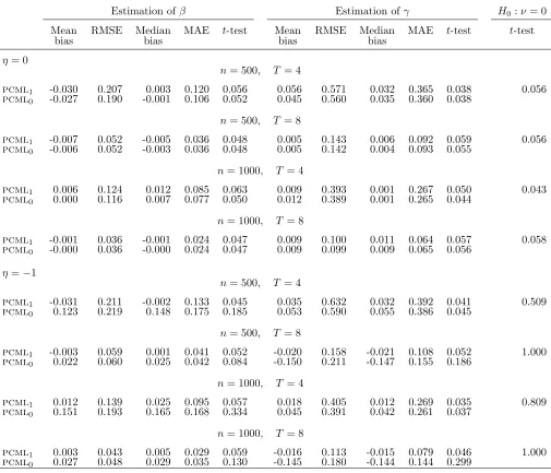
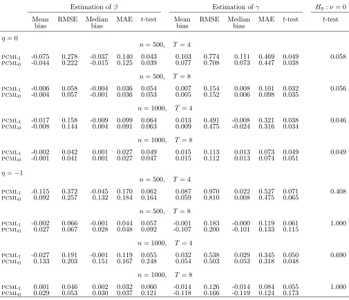
Tables 5 and 6 report the simulation results for two departures from the benchmark design: Table 5 refers to a binary covariate generated by a normal link function, while Table 6 refers to a normally distributed covariate depending on the time-varying covariate

vit (see Section 5.1 for details). These exercises are meant to investigate the properties of the pcml estimator when assumption (17) does not hold and the model formulated in Theorem 3 just embeds a linear approximation of (17). When the covariate is binary, the bias of the pcml1 estimator of β and γ is always negligible. As for efficiency, the RMSE

[image:22.612.60.564.192.627.2]

Table 1: Normally distributed covariate,β = 0, γ = 0, ψ = 0

Estimation ofβ Estimation ofγ H0:ν= 0

Mean RMSE Median MAE t-test Mean RMSE Median MAE t-test t-test

bias bias bias bias

η= 0

n= 500, T= 4

pcml1 -0.003 0.072 -0.003 0.048 0.052 -0.026 0.305 -0.031 0.210 0.039 0.051

pcml0 -0.001 0.060 0.001 0.039 0.045 -0.027 0.302 -0.025 0.209 0.036

n= 500, T= 8

pcml1 -0.000 0.027 0.000 0.018 0.066 0.003 0.106 0.002 0.073 0.055 0.037

pcml0 -0.000 0.027 -0.000 0.018 0.062 0.003 0.106 0.002 0.073 0.056

n= 1000, T = 4

pcml1 0.000 0.051 -0.000 0.034 0.051 0.002 0.224 0.009 0.143 0.055 0.050

pcml0 -0.000 0.043 -0.001 0.029 0.052 0.002 0.223 0.010 0.143 0.052

n= 1000, T = 8

pcml1 0.001 0.019 0.001 0.012 0.048 0.000 0.074 -0.002 0.048 0.053 0.055

pcml0 0.001 0.018 0.001 0.012 0.053 0.000 0.074 -0.002 0.048 0.053

η=−1

n= 500, T = 4

pcml1 0.002 0.078 -0.001 0.054 0.042 -0.013 0.338 -0.009 0.224 0.045 0.984

pcml0 0.155 0.167 0.154 0.154 0.694 0.138 0.346 0.152 0.236 0.057

n= 500, T = 8

pcml1 -0.003 0.027 -0.002 0.018 0.047 -0.000 0.112 -0.000 0.076 0.044 1.000

pcml0 0.048 0.054 0.048 0.048 0.498 0.053 0.115 0.049 0.078 0.078

n= 1000, T = 4

pcml1 -0.002 0.053 -0.002 0.037 0.051 -0.003 0.245 -0.002 0.166 0.055 1.000

pcml0 0.149 0.155 0.149 0.149 0.935 0.149 0.275 0.153 0.195 0.089

n= 1000, T = 8

pcml1 -0.003 0.020 -0.004 0.014 0.071 0.004 0.080 0.003 0.055 0.046 1.000

[image:23.612.60.564.193.627.2]

Table 2: Normally distributed covariate,β =₋1,γ = 0, ψ = 0

Estimation ofβ Estimation ofγ H0:ν= 0

Mean RMSE Median MAE t-test Mean RMSE Median MAE t-test t-test

bias bias bias bias

η= 0

n= 500, T= 4

pcml1 -0.049 0.178 -0.027 0.106 0.039 0.037 0.482 0.028 0.325 0.056 0.055

pcml0 -0.039 0.165 -0.020 0.102 0.048 0.033 0.473 0.018 0.318 0.056

n= 500, T= 8

pcml1 -0.007 0.049 -0.005 0.034 0.057 -0.006 0.135 -0.000 0.095 0.049 0.045

pcml0 -0.007 0.049 -0.004 0.033 0.056 -0.006 0.134 -0.001 0.094 0.053

n= 1000, T = 4

pcml1 -0.019 0.117 -0.005 0.075 0.043 0.005 0.309 0.010 0.219 0.041 0.037

pcml0 -0.015 0.111 -0.007 0.073 0.046 0.006 0.307 0.007 0.222 0.042

n= 1000, T = 8

pcml1 -0.001 0.035 0.001 0.023 0.051 0.005 0.090 0.006 0.060 0.040 0.056

pcml0 -0.001 0.035 0.001 0.022 0.055 0.005 0.090 0.007 0.060 0.041

η=−1

n= 500, T= 4

pcml1 -0.058 0.208 -0.037 0.122 0.058 -0.015 0.501 -0.020 0.333 0.051 0.808

pcml0 0.122 0.199 0.138 0.158 0.222 0.045 0.474 0.058 0.317 0.050

n= 500, T = 8

pcml1 -0.006 0.055 -0.005 0.035 0.049 0.002 0.148 0.002 0.101 0.058 1.000

pcml0 0.047 0.069 0.048 0.052 0.194 -0.097 0.170 -0.095 0.122 0.112

n= 1000, T = 4

pcml1 -0.027 0.134 -0.018 0.082 0.060 -0.003 0.340 -0.003 0.224 0.049 0.981

pcml0 0.140 0.177 0.148 0.150 0.330 0.055 0.325 0.043 0.213 0.051

n= 1000, T = 8

pcml1 -0.003 0.039 -0.003 0.027 0.056 0.007 0.101 0.007 0.069 0.055 1.000

[image:24.612.60.564.193.626.2]

Table 3: Normally distributed covariate,β = 0, γ = 1, ψ = 0

Estimation ofβ Estimation ofγ H0:ν= 0

Mean RMSE Median MAE t-test Mean RMSE Median MAE t-test t-test

bias bias bias bias

η= 0

n= 500, T= 4

pcml1 -0.002 0.079 0.001 0.051 0.033 -0.003 0.418 -0.000 0.289 0.063 0.040

pcml0 -0.000 0.069 -0.003 0.046 0.025 -0.010 0.412 -0.013 0.288 0.060

n= 500, T= 8

pcml1 -0.002 0.027 -0.003 0.018 0.049 0.005 0.113 0.004 0.076 0.048 0.052

pcml0 -0.002 0.027 -0.003 0.017 0.049 0.005 0.113 0.003 0.075 0.046

n= 1000, T = 4

pcml1 -0.003 0.054 -0.003 0.037 0.031 -0.025 0.279 -0.029 0.195 0.052 0.035

pcml0 -0.002 0.048 -0.000 0.032 0.045 -0.029 0.277 -0.033 0.193 0.049

n= 1000, T = 8

pcml1 -0.001 0.020 -0.000 0.014 0.051 -0.001 0.080 -0.006 0.054 0.049 0.059

pcml0 -0.001 0.020 -0.000 0.014 0.051 -0.002 0.080 -0.005 0.054 0.048

η=−1

n= 500, T= 4

pcml1 0.006 0.085 0.008 0.056 0.037 -0.004 0.441 -0.016 0.297 0.050 0.894

pcml0 0.143 0.157 0.143 0.143 0.520 0.147 0.442 0.140 0.281 0.055

n= 500, T = 8

pcml1 0.007 0.031 0.006 0.021 0.065 0.006 0.125 0.003 0.084 0.057 1.000

pcml0 0.018 0.032 0.017 0.022 0.104 0.008 0.114 0.002 0.078 0.055

n= 1000, T = 4

pcml1 0.004 0.060 0.005 0.042 0.039 -0.001 0.301 -0.002 0.191 0.059 0.992

pcml0 0.139 0.147 0.137 0.137 0.815 0.148 0.323 0.147 0.225 0.075

n= 1000, T = 8

pcml1 0.004 0.020 0.003 0.013 0.059 0.002 0.089 0.004 0.060 0.055 1.000

[image:25.612.56.561.195.628.2]

Table 4: Normally distributed covariate,β =₋1,γ = 1, ψ = 0

Estimation ofβ Estimation ofγ H0:ν= 0

Mean RMSE Median MAE t-test Mean RMSE Median MAE t-test t-test

bias bias bias bias

η= 0

n= 500, T= 4

pcml1 -0.030 0.207 0.003 0.120 0.056 0.056 0.571 0.032 0.365 0.038 0.056

pcml0 -0.027 0.190 -0.001 0.106 0.052 0.045 0.560 0.035 0.360 0.038

n= 500, T= 8

pcml1 -0.007 0.052 -0.005 0.036 0.048 0.005 0.143 0.006 0.092 0.059 0.056

pcml0 -0.006 0.052 -0.003 0.036 0.048 0.005 0.142 0.004 0.093 0.055

n= 1000, T = 4

pcml1 0.006 0.124 0.012 0.085 0.063 0.009 0.393 0.001 0.267 0.050 0.043

pcml0 0.000 0.116 0.007 0.077 0.050 0.012 0.389 0.001 0.265 0.044

n= 1000, T = 8

pcml1 -0.001 0.036 -0.001 0.024 0.047 0.009 0.100 0.011 0.064 0.057 0.058

pcml0 -0.000 0.036 -0.000 0.024 0.047 0.009 0.099 0.009 0.065 0.056

η=−1

n= 500, T = 4

pcml1 -0.031 0.211 -0.002 0.133 0.045 0.035 0.632 0.032 0.392 0.041 0.509

pcml0 0.123 0.219 0.148 0.175 0.185 0.053 0.590 0.055 0.386 0.045

n= 500, T = 8

pcml1 -0.003 0.059 0.001 0.041 0.052 -0.020 0.158 -0.021 0.108 0.052 1.000

pcml0 0.022 0.060 0.025 0.042 0.084 -0.150 0.211 -0.147 0.155 0.186

n= 1000, T = 4

pcml1 0.012 0.139 0.025 0.095 0.057 0.018 0.405 0.012 0.269 0.035 0.809

pcml0 0.151 0.193 0.165 0.168 0.334 0.045 0.391 0.042 0.261 0.037

n= 1000, T = 8

pcml1 0.003 0.043 0.005 0.029 0.059 -0.016 0.113 -0.015 0.079 0.046 1.000

[image:26.612.60.564.192.627.2]

Table 5: Binary covariate, β =₋1, γ = 1, ψ = 0

Estimation ofβ Estimation ofγ H0:ν= 0

Mean RMSE Median MAE t-test Mean RMSE Median MAE t-test t-test

bias bias bias bias

η= 0

n= 500, T= 4

pcml1 -0.007 0.352 -0.005 0.242 0.040 0.005 0.398 0.009 0.263 0.049 0.045

pcml0 -0.011 0.309 0.001 0.210 0.038 -0.003 0.390 0.004 0.260 0.048

n= 500, T= 8

pcml1 -0.010 0.116 -0.010 0.078 0.050 0.000 0.113 -0.002 0.076 0.053 0.060

pcml0 -0.008 0.115 -0.009 0.076 0.049 0.000 0.113 -0.001 0.076 0.051

n= 1000, T = 4

pcml1 0.019 0.238 0.023 0.160 0.042 -0.018 0.279 -0.029 0.187 0.060 0.045

pcml0 -0.000 0.211 0.003 0.140 0.040 -0.019 0.277 -0.033 0.187 0.057

n= 1000, T = 8

pcml1 -0.009 0.080 -0.012 0.054 0.049 0.004 0.079 0.002 0.054 0.040 0.065

pcml0 -0.008 0.079 -0.010 0.053 0.047 0.004 0.079 0.001 0.054 0.040

η=−1

n= 500, T= 4

pcml1 0.022 0.364 0.038 0.236 0.044 0.001 0.409 -0.007 0.278 0.048 0.579

pcml0 0.432 0.528 0.447 0.449 0.309 0.042 0.399 0.029 0.267 0.052

n= 500, T = 8

pcml1 0.008 0.121 0.005 0.083 0.047 -0.003 0.116 -0.009 0.080 0.048 1.000

pcml0 0.049 0.124 0.046 0.080 0.074 -0.024 0.114 -0.027 0.083 0.049

n= 1000, T = 4

pcml1 0.044 0.265 0.063 0.185 0.048 -0.022 0.290 -0.032 0.193 0.052 0.883

pcml0 0.447 0.494 0.450 0.451 0.553 0.029 0.283 0.018 0.189 0.055

n= 1000, T = 8

pcml1 0.013 0.088 0.014 0.057 0.063 -0.001 0.081 0.002 0.055 0.043 1.000

[image:27.612.56.561.195.628.2]

Table 6: Normally distributed covariate, β=₋1, γ = 1, ψ = 0.5

Estimation ofβ Estimation ofγ H0:ν= 0

Mean RMSE Median MAE t-test Mean RMSE Median MAE t-test t-test

bias bias bias bias

η= 0

n= 500, T= 4

pcml1 -0.075 0.278 -0.037 0.140 0.043 0.103 0.774 0.111 0.469 0.049 0.058

pcml0 -0.044 0.222 -0.015 0.125 0.039 0.077 0.708 0.073 0.447 0.038

n= 500, T= 8

pcml1 -0.006 0.058 -0.004 0.036 0.054 0.007 0.154 0.008 0.101 0.032 0.056

pcml0 -0.004 0.057 -0.001 0.036 0.053 0.005 0.152 0.006 0.098 0.035

n= 1000, T = 4

pcml1 -0.017 0.158 -0.009 0.099 0.064 0.013 0.491 -0.008 0.321 0.038 0.046

pcml0 -0.008 0.144 0.004 0.091 0.063 0.009 0.475 -0.024 0.316 0.034

n= 1000, T = 8

pcml1 -0.002 0.042 0.001 0.027 0.049 0.015 0.113 0.013 0.073 0.049 0.049

pcml0 -0.001 0.041 0.001 0.027 0.047 0.015 0.112 0.013 0.074 0.051

η=−1

n= 500, T= 4

pcml1 -0.115 0.372 -0.045 0.170 0.062 0.087 0.970 0.022 0.527 0.071 0.408

pcml0 0.092 0.257 0.132 0.184 0.164 0.059 0.810 0.008 0.475 0.065

n= 500, T = 8

pcml1 -0.002 0.066 -0.001 0.044 0.057 -0.001 0.183 -0.000 0.119 0.061 1.000

pcml0 0.027 0.067 0.028 0.048 0.092 -0.107 0.200 -0.101 0.133 0.115

n= 1000, T = 4

pcml1 -0.027 0.191 -0.001 0.119 0.055 0.032 0.538 0.029 0.345 0.050 0.690

pcml0 0.133 0.203 0.151 0.167 0.248 0.054 0.503 0.053 0.318 0.048

n= 1000, T = 8

pcml1 0.001 0.046 0.002 0.032 0.060 -0.014 0.126 -0.014 0.084 0.055 1.000

5.3

Comparison with alternative estimators

We compare the performance of the pcml estimator for model (18) with two alternative approaches. The first, denoted by W, is the correlated random-effects approach based on the proposal by Wooldridge (2005) for nonlinear dynamic panel data models, where the individual unobserved heterogeneity is assumed to be normally distributed and ini-tial conditions are handled by specifying the distribution of ci conditional on the initial value of yi. In Wooldridge (2005) a general formulation for this conditional distribution

is proposed, where the individual random effects are allowed to depend on linear combi-nations of time-averages of strictly exogenous covariates (Mundlak, 1978). We specify the following conditional distribution of ci

ci_|yi1 ∼yi1α+ ¯viπ+c∗_i, c∗_i ∼N(0, σ 2

c), i= 1, . . . , n.

where ¯vi = (1/T)PT

t=1vit. It is worth noting that, in this case, the ml estimator of the

model parameters is consistent ifc∗

i is independent of the possibly predetermined covariate xit. Therefore, we generate samples where ci in (30) is distributed as a normal random variable with zero mean, unit variance, and̟ = 0, in order to avoid the misspecification of the random effects. Nevertheless we also compare the ml and pcml estimator in the scenario where the individual intercepts are generated as in (30).

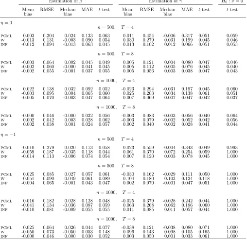
The second is the so-called infeasible logit estimator (Honor´e and Kyriazidou, 2000) denoted by inf, where the generated individual intercepts are used as an additional co-variate and the model parameters are then estimated by ml based on the pooled logit model formulation. The purpose is to compare the pcml estimator with a benchmark that is not sensitive to substantial deviations from the approximating model (20).

[image:29.612.57.565.168.662.2]

Table 7: Normally distributed covariate, β =₋1, γ = 1, ci _∼N(0,1), ̟ = 0

Estimation ofβ Estimation ofγ H0:ν= 0

Mean RMSE Median MAE t-test Mean RMSE Median MAE t-test t-test

bias bias bias bias

η= 0

n= 500, T= 4

pcml 0.003 0.204 0.024 0.133 0.063 0.011 0.454 -0.006 0.317 0.051 0.059

w -0.013 0.131 -0.003 0.090 0.054 0.030 0.279 0.031 0.199 0.045 0.046

inf -0.012 0.094 -0.013 0.063 0.045 0.013 0.102 0.012 0.066 0.051 0.053

n= 500, T= 8

pcml -0.003 0.064 0.002 0.045 0.049 0.005 0.121 0.004 0.080 0.047 0.046

w -0.002 0.060 -0.000 0.041 0.045 0.005 0.112 0.005 0.076 0.045 0.040

inf -0.002 0.055 -0.001 0.037 0.055 0.005 0.056 0.003 0.038 0.047 0.043

n= 1000, T = 4

pcml 0.022 0.138 0.032 0.092 0.052 -0.023 0.294 -0.031 0.197 0.045 0.060

w -0.003 0.095 0.004 0.065 0.060 0.025 0.203 0.034 0.138 0.061 0.051

inf -0.005 0.070 -0.003 0.047 0.064 0.007 0.069 0.007 0.047 0.042 0.037

n= 1000, T = 8

pcml -0.000 0.046 -0.000 0.032 0.056 -0.003 0.083 -0.003 0.056 0.040 0.064

w 0.002 0.042 0.003 0.028 0.062 -0.003 0.079 -0.002 0.052 0.042 0.056

inf 0.002 0.038 0.001 0.024 0.057 0.002 0.040 0.002 0.028 0.041 0.044

η=−1

n= 500, T= 4

pcml -0.010 0.279 0.020 0.173 0.058 0.023 0.559 -0.004 0.343 0.049 0.993

w -0.059 0.187 -0.035 0.118 0.044 0.061 0.370 0.072 0.254 0.059 1.000

inf -0.014 0.113 -0.006 0.074 0.054 0.007 0.120 0.003 0.078 0.045 1.000

n= 500, T= 8

pcml 0.025 0.085 0.027 0.057 0.061 -0.030 0.162 -0.029 0.111 0.050 1.000

w -0.051 0.090 -0.049 0.061 0.089 0.104 0.180 0.103 0.124 0.118 1.000

inf -0.004 0.065 -0.001 0.043 0.047 0.002 0.070 -0.001 0.047 0.051 1.000

n= 1000, T = 4

pcml 0.016 0.182 0.028 0.128 0.048 -0.025 0.379 -0.028 0.242 0.044 1.000

w -0.041 0.134 -0.036 0.087 0.059 0.063 0.268 0.062 0.186 0.060 1.000

inf -0.010 0.081 -0.009 0.055 0.055 0.011 0.085 0.011 0.057 0.044 1.000

n= 1000, T = 8

pcml 0.025 0.064 0.026 0.044 0.077 -0.038 0.121 -0.038 0.080 0.071 1.000

w -0.050 0.073 -0.050 0.053 0.148 0.096 0.143 0.098 0.105 0.165 1.000

[image:30.612.55.562.165.663.2]

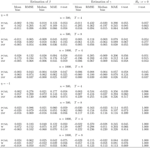
Table 8: Normally distributed covariate, β=₋1, γ = 1, ci = (1/T)P4 t=1x

∗

it, ̟ = 0.5

Estimation ofβ Estimation ofγ H0:ν= 0

Mean RMSE Median MAE t-test Mean RMSE Median MAE t-test t-test

bias bias bias bias

η= 0

n= 500, T= 4

pcml -0.002 0.194 0.018 0.123 0.053 -0.011 0.432 -0.020 0.290 0.055 0.057

w 0.162 0.205 0.167 0.169 0.311 -0.205 0.362 -0.197 0.245 0.085 0.663

inf -0.011 0.098 -0.008 0.066 0.058 0.016 0.094 0.015 0.064 0.049 0.065

n= 500, T= 8

pcml -0.011 0.065 -0.009 0.045 0.052 0.005 0.118 0.003 0.078 0.041 0.054

w 0.056 0.082 0.058 0.061 0.183 -0.061 0.125 -0.064 0.089 0.067 0.277

inf -0.005 0.054 -0.006 0.036 0.051 0.005 0.056 0.005 0.038 0.055 0.050

n= 1000, T = 4

pcml 0.028 0.132 0.038 0.094 0.058 -0.010 0.305 -0.009 0.206 0.056 0.051

w 0.173 0.194 0.176 0.176 0.547 -0.196 0.289 -0.193 0.212 0.148 0.915

inf -0.005 0.068 -0.006 0.045 0.059 0.006 0.067 0.009 0.045 0.058 0.053

n= 1000, T = 8

pcml -0.003 0.043 -0.004 0.028 0.047 0.006 0.088 0.004 0.057 0.058 0.045

w 0.063 0.074 0.062 0.062 0.325 -0.060 0.100 -0.060 0.070 0.124 0.488

inf -0.000 0.037 -0.000 0.025 0.037 0.000 0.039 -0.000 0.026 0.051 0.037

η=−1

n= 500, T= 4

pcml 0.002 0.276 0.021 0.177 0.058 0.003 0.534 -0.023 0.356 0.039 0.996

w 0.057 0.200 0.072 0.143 0.101 0.007 0.416 0.037 0.293 0.060 1.000

inf -0.068 0.130 -0.068 0.083 0.074 0.229 0.255 0.226 0.226 0.517 1.000

n= 500, T= 8

pcml 0.023 0.086 0.021 0.060 0.059 -0.030 0.163 -0.033 0.114 0.055 1.000

w -0.020 0.079 -0.016 0.055 0.062 0.060 0.158 0.058 0.107 0.073 1.000

inf -0.016 0.069 -0.016 0.046 0.056 0.117 0.135 0.116 0.116 0.399 1.000

n= 1000, T = 4

pcml 0.023 0.183 0.040 0.122 0.050 -0.022 0.370 -0.028 0.245 0.045 1.000

w 0.072 0.152 0.075 0.107 0.129 0.007 0.298 0.011 0.203 0.066 1.000

inf -0.063 0.102 -0.060 0.070 0.114 0.222 0.236 0.220 0.220 0.814 1.000

n= 1000, T = 8

pcml 0.024 0.062 0.025 0.042 0.075 -0.029 0.115 -0.032 0.084 0.059 1.000

w -0.021 0.057 -0.022 0.039 0.056 0.057 0.116 0.058 0.081 0.076 1.000

6

Conclusions

In this paper, we propose a novel model formulation for dynamic binary panel data models that accounts for feedback effects from the past of the outcome variable on the present value of covariates. Our proposal is particularly well suited for short panels with a large number of cross-section units, typically provided by rotated or strongly unbalanced continuous surveys, often employed for microeconomic applications. Our formulation is based on the equivalence between Granger’s definition of noncausality and a modification of the Sims’ strict exogeneity assumption for nonlinear panel data models, introduced by Chamberlain (1982) and for which we provide a more general theorem.

Under the logit model, the proposed model formulation yields three main advantages compared to the few available alternatives: (i) it does not require the specification of a parametric model for the predetermined explanatory variables; (ii) it has a simple formu-lation and allows, in practice, for the inclusion of a large number of predetermined covari-ates, discrete or continuous; (iii) its parameters can be estimated within a fixed-effects approach by a pcml, thereby allowing for an arbitrary dependence structure between the model covariates and the individual permanent unobserved heterogeneity.

From our simulation results, it emerges that pcml provides consistent estimation of the regression and state dependence parameters in presence of substantial departures from noncausality and that the bias is negligible even when the conditions for the exact logit model formulation are violated. Furthermore, we show that the alternative random-effects ml estimator based on Wooldridge (2005) for the model here proposed exhibits comparable finite-sample properties, provided the dependence between the predetermined covariate and the unobserved heterogeneity is reliably accounted for.

References

Akay, A. (2012). Finite-sample comparison of alternative methods for estimating dynamic panel data models. Journal of Applied Econometrics, 27(7):1189–1204.

Alessie, R., Hochguertel, S., and van Soest, A. (2004). Ownership of Stocks and Mutual Funds: A Panel Data Analysis.The Review of Economics and Statistics, 86(3):783–796.

Anderson, T. W. and Hsiao, C. (1981). Estimation of dynamic models with error compo-nents. Journal of the American statistical Association, 76(375):598–606.

Arellano, M. and Bond, S. (1991). Some tests of specification for panel data: Monte carlo evidence and an application to employment equations. The review of economic studies, 58(2):277–297.

Arellano, M. and Bover, O. (1995). Another look at the instrumental variable estimation of error-components models. Journal of econometrics, 68(1):29–51.

Arellano, M. and Carrasco, R. (2003). Binary choice panel data models with predeter-mined variables. Journal of Econometrics, 115(1):125–157.

Arulampalam, W. (2002). State dependence in unemployment incidence: evidence for british men revisited. Technical report, IZA Discussion paper series.

Barndorff-Nielsen, O. (1978). Information and exponential families in statistical theory. John Wiley & Sons.

Bartolucci, F. and Nigro, V. (2010). A dynamic model for binary panel data with unob-served heterogeneity admitting a √n-consistent conditional estimator. Econometrica, 78:719–733.

Bartolucci, F. and Nigro, V. (2012). Pseudo conditional maximum likelihood estimation of the dynamic logit model for binary panel data. Journal of Econometrics, 170:102–116.

Bartolucci, F. and Pigini, C. (2016). cquad: An R and Stata package for conditional max-imum likelihood estimation of dynamic binary panel data models. Journal of Statistical Software, In press.

Bettin, G. and Lucchetti, R. (2016). Steady streams and sudden bursts: persistence patterns in remittance decisions. Journal of Population Economics, 29(1):263–292.

Blundell, R. and Bond, S. (1998). Initial conditions and moment restrictions in dynamic panel data models. Journal of econometrics, 87(1):115–143.

Brown, S., Ghosh, P., and Taylor, K. (2014). The existence and persistence of house-hold financial hardship: A bayesian multivariate dynamic logit framework. Journal of Banking & Finance, 46:285–298.

Cappellari, L. and Jenkins, S. P. (2004). Modelling low income transitions. Journal of Applied Econometrics, 19(5):593–610.

Carrasco, R. (2001). Binary choice with binary endogenous regressors in panel data.

Journal of Business & Economic Statistics, 19(4):385–394.

Carro, J. M. and Traferri, A. (2012). State dependence and heterogeneity in health using a bias-corrected fixed-effects estimator. Journal of Applied Econometrics, 29(2):181–207.

Chamberlain, G. (1980). Analysis of covariance with qualitative data. The Review of Economic Studies, 47(1):225–238.

Chamberlain, G. (1982). The general equivalence of granger and sims causality. Econo-metrica: Journal of the Econometric Society, 50(3):569–581.

Chamberlain, G. (1984). Panel data. Handbook of Econometrics, 2:1247–1318.

Chamberlain, G. (1985). Heterogeneity, omitted variable bias, and duration dependence. In Heckman, J. J. and Singer, B., editors, Longitudinal Analysis of Labor Market Data. Cambridge University Press: Cambridge.

Contoyannis, P., Jones, A. M., and Rice, N. (2004). Simulation-based inference in dynamic panel probit models: an application to health. Empirical Economics, 29(1):49–77.

Cox, D. (1972). The analysis of multivariate binary data. Applied statistics, 21(2):113–120.

Florens, J.-P. and Mouchart, M. (1982). A note on noncausality. Econometrica: Journal of the Econometric Society, 50(3):583–591.

Giarda, E. (2013). Persistency of financial distress amongst italian households: Evidence from dynamic models for binary panel data. Journal of Banking & Finance, 37(9):3425 – 3434.

Granger, C. W. (1969). Investigating causal relations by econometric models and cross-spectral methods. Econometrica: Journal of the Econometric Society, 37(3):424–438.

Hansen, L. P. (1982). Large sample properties of generalized method of moments estima-tors. Econometrica: Journal of the Econometric Society, 50(4):1029–1054.

Heckman, J. J. (1981). Heterogeneity and state dependence. Structural Analysis of Dis-crete Data with Econometric Applications, MIT Press: Cambridge MA. Manski CF, McFadden (eds).

Heckman, J. J. and Borjas, G. J. (1980). Does unemployment cause future unemployment? definitions, questions and answers from a continuous time model of heterogeneity and state dependence. Economica, 47(187):pp. 247–283.

Heiss, F. (2011). Dynamics of self-rated health and selective mortality. Empirical eco-nomics, 40(1):119–140.

Honor´e, B. E. and Kyriazidou, E. (2000). Panel data discrete choice models with lagged dependent variables. Econometrica, 68(4):839–874.

Honor´e, B. E. and Lewbel, A. (2002). Semiparametric binary choice panel data models without strictly exogeneous regressors. Econometrica, 70(5):2053–2063.

Hsiao, C. (2005). Analysis of Panel Data. Cambridge University Press, New York, 2nd edition.

Hyslop, D. R. (1999). State dependence, serial correlation and heterogeneity in intertem-poral labor force participation of married women. Econometrica, 67(6):1255–1294.

Keane, M. P. and Sauer, R. M. (2009). Classification error in dynamic discrete choice models: Implications for female labor supply behavior. Econometrica, 77(3):975–991.

Michaud, P.-C. and Tatsiramos, K. (2011). Fertility and female employment dynamics in europe: the effect of using alternative econometric modeling assumptions. Journal of Applied Econometrics, 26(4):641–668.

Mosconi, R. and Seri, R. (2006). Non-causality in bivariate binary time series. Journal of Econometrics, 132(2):379–407.

Mundlak, Y. (1978). On the Pooling of Time Series and Cross Section Data.Econometrica, 46(1):69–85.

Pigini, C., Presbitero, A. F., and Zazzaro, A. (2016). State dependence in access to credit.

Journal of Financial Stability, pages –. forthcoming.

Stewart, M. B. (2007). The interrelated dynamics of unemployment and low-wage em-ployment. Journal of Applied Econometrics, 22(3):511–531.

Wooldridge, J. M. (2000). A framework for estimating dynamic, unobserved effects panel data models with possible feedback to future explanatory variables. Economics Letters, 68(3):245–250.

Wooldridge, J. M. (2005). Simple solutions to the initial conditions problem in dynamic, nonlinear panel data models with unobserved heterogeneity. Journal of Applied Econo-metrics, 20(1):39–54.

Wooldridge, J. M. (2010). Econometric analysis of cross section and panel data. The MIT press.