Munich Personal RePEc Archive
Corruption vs reforms: Why do voters
prefer the former?
Fedotenkov, Igor
Russian Presidential Academy of National Economy and Public
Administration
18 October 2018
Online at
https://mpra.ub.uni-muenchen.de/89581/
Corruption vs reforms:
Why do voters prefer the
former?
Igor Fedotenkov
1
Abstract
In this paper, we address the question of why voters tolerate corrupt politi-cians. Standard economic techniques such as expected utility maximization under uncertainty are employed. We show that a corrupt politician is less likely to institute reforms which can cause short-term losses for voters during a tran-sitional period or lead with some probability to non-success. Voters’ higher risk aversion causes an increased fear of reforms and higher tolerance for corruption. We also show that during an economic crisis the corruptionists’ optimal strat-egy is not to institute reforms, as models with honest politicians predict, but to reduce the level of corruption. Using panel data techniques, we show that such a strategy is in line with the empirical CIS data; however, it follows with a short delay.
JEL Classification: D72, D73, E60, I38.
Keywords: Corruption; politician; median voter; reforms; risk aversion.
1
1
Introduction
Corruption affects agents’ wellbeing and macroeconomic indicators. It is one of the main obstacles to economic growth (Mauro 1995; Del Monte and Papagni 2001). As a result, the causes and consequences of corruption have attracted much attention from economists, sociologists and political scientists. One of the central questions in studying the phenomenon of corruption is why peo-ple elect corrupt politicians. Numerous explanations have been proposed and ideas discussed. We address this question using standard economic techniques, such as utility maximization under uncertainty. We show that if agents are sufficiently risk averse or the intertemporal substitution of consumption is low, agents may not desire reforms, because their effects are uncertain or produce losses in the short run. Therefore, agents often prefer to elect corrupt politi-cians who steal a part of the agents’ endowments, but have fewer incentives for implementing reforms and, therefore, offer stability. Furthermore, we show that corrupt politicians’ optimal strategy during an economic crisis is not to activate economic reforms, as predicted in models with honest politicians (Vis 2009; Hol-landers and Vis 2013), but to steal less. Using the data of the Commonwealth of Independent States (CIS), we show that such a policy takes place in practice, but adjustments in corruption follow economic growth with a 1-2 year lag.
Many studies emphasize that a higher level of democracy is associated with lower corruption. Political freedom, freedom of speech and fair elections give voters an opportunity to punish corrupt politicians and elect the honest (Gold-smith 1999; Chowdhury 2004; Sung 2004). Nevertheless, corruption exists in democratic countries as well, and democracy enables some forms of corruption, which are not possible under a dictatorship (Moran 2001). So, why do voters in democratic countries continue to elect corrupt politicians? The explanations are multiple.
One hypothesis is that in democratic countries people tend not to elect corrupt politicians; however, information about their corrupt activities may not be public. The government may influence news content by maintaining a “cozy” relationship with the media even in the absence of censorship (Besley and Prat 2006). Therefore, if corruption is uncovered, the ability to attract and hold the public’s attention may be limited (Winters and Weitz-Shapiro 2013). Another problem, related to the dissemination of information is that often voters do not believe information about corruption. Despite receiving such information, voters may discard it as not credible (Mu˜noz, Anduiza, and Gallego 2016) or assign blame incorrectly (Kurer 2002; De Vries and Solaz 2017).
to a wider choice in this part of the political spectrum or they choose not par-ticipate in elections. However, if the number of political parties is large, the U-shape relationship becomes flatter (Charron and B˚agenholm 2016). Apart from the absolute number of political parties, their quality also matters. Often voters tend not to punish a corrupt party if they believe that alternative parties are also corrupt (Cordero and Blais 2017).
Another common explanation of why voters choose corrupt politicians is that they create clientelistic networks and deliver public goods to them. They manipulate public goods and resources so that political loyalty is rewarded. Put simply, corrupt officials buy public support (Kurer 2002; Manzetti and Wilson 2007; Pereira and Melo 2015). However, not all studies confirm this explanation. Using data from Greece, Konstantinidis and Xezonakis (2013) found that the clientalistic exchange has negative effects on the public support of a corrupt politician, while the popularity of corrupt politicians increases if they provide collective benefits, such as lower taxes. This argument was also indirectly confirmed by Mu˜noz et al. (2016) on Catalonian data.
Our paper proposes another motive for voting for corrupt officials. We note that if we introduce corrupt politicians to a model with unpopular reforms, agents may tolerate corruption, because corrupt politicians have fewer incentives to institute reforms. This is so if politicians’ benefits from corruption exceed the benefits obtained from economic reforms. To the best of our knowledge, this is the first paper linking the political economy of unpopular reforms with corruption.
Our model relies on the assumption of fear of reforms. This is a quite realis-tic assumption in Russia and other post-Soviet countries. According to RLMS data, approximately 55 percent of Russians claimed that their lives have wors-ened since economic reforms started in 1991, with only 23 percent holding the opposite opinion in 2006 (Denisova, Eller, and Zhuravskaya 2010). These re-sults are not surprising. Having analysed post-communist transitions in Eastern European countries, Hellman (1998) found that partial reforms are profitable for small groups of people and create large losses for the rest. Therefore, the optimal winners’ strategy is to freeze the economy in a partial reform equilib-rium that is profitable to them, while imposing substantial costs on the rest of the population. Such partial reforms were implemented in a number of Eastern European countries, including Russia in the nineties.
Even if economic reforms are complete, they often create losses in the short run: e.g., a switch from a pay-as-you go to a more funded pension scheme (Breyer 1989), capital taxation (Peterman 2013; Fehr and Kindermann 2015), sector-specific labour and capital taxations (Fedotenkov 2018), a switch from VAT to consumption taxes (Sarkar and Zodrow 1993). The advantages of the reforms are also received unevenly by different groups, and some groups become worse off even in the long run (Bucciol et al. 2017). Consequently, even in Western economies, the majority often prefers the status quo (Boeri, B¨orsch-Supan, and Tabellini 2002; Brooks and Manza 2006; Van Groezen, Kiiver, and Unger 2009).
Vis (2013) to study the timing of reforms. Their model includes two politicians who receive benefits (sometimes immaterial) when they implement reforms and the median voter who receives direct losses. If a politician implements a reform, next election cycle, the voter chooses another politician. The voter also at-tributes the responsibility for economic crises to the government, and if a crisis hits, she then elects a different politician. Therefore, the optimal strategy for a politician in office is to implement reforms only when a crisis hits. We take this model as a starting point, but include possibilities for corruption. We simplify politicians’ behavior, which does not affect our main results; however, the be-havior of the median voter is more complicated, because now she needs not only to elect a politician, but also make decisions about the upper level of tolerated corruption. If the crisis hits, similarly to Hollanders and Vis, the median voter wishes to punish the politician for bad economic performance. However, the corrupt politician can mitigate the losses of the median voter by reducing the level of corruption and so remain in office. Similar politicians’ behaviour was found empirically in the CIS countries.
The remaining part of the paper is designed as follows. In the next section, we develop a theoretical model. Section 3 provides some empirical cross-country estimates, which confirm the main mechanism of the model. In section 4, predic-tions of the model are validated empirically using panel data technique. Finally, section 5 concludes.
2
Model
There are three players in the model living forever: two politicians and one median voter. The total population is clearly larger, so we suppose that its size is equal toN. In each period, only one politician holds elected office, chosen by the median voter.
There is an infinite set of reforms, and each period, a politician in office may (or may not) implement one of them. For now, we assume that the median voter dislikes reforms. The formal condition, when this is the case, is derived later. If a politician implements a reform, next period, another politician is elected. If the reform is not implemented, the same politician is reelected next period.2 We suppose that all players have perfect information concerning the
other players and their preferences.
2.1
Politicians
Each period the politician in office makes one decision:
• He decides whether to institute a reform or not.
2
This action is performed depending on the maximization of his utility function. At timet= 0, this utility function is given by
V0=
∞
X
i=0 δiv(x
i), (1)
whereδ is a discount rate, 0< δ <1,U(·) is a strictly concave instantaneous utility function andxi denotes consumption at timei,v(xi)>0 forxi>0 and
v(xi) = 0 whenxi= 0.
If a politician is not in office his benefit in this period is equal to zerow= 0, otherwise he receives legal benefits w, w > 0. If he undertakes a reform, he obtains satisfaction from the reformr,r≥0 (if the reform is not made,r= 0). If voters wish, they may allow politicians to steal the amounts of resources, and the politician does it. In this case, losses from corruption are allocated evenly between agents. The difference between benefits from corruption and lawful benefits is that the former lead to direct losses for the median voter. All benefits received by politicians are consumed in the same period.
Next, we simplify the analysis of Hollanders and Vis by assuming that politicians have perfect information about each other and take this informa-tion into account when making their decisions. Having used the sums of ge-ometric sequences, we find that a politician’s utility of never reforming and always staying in office is given by Vn
0 = (1−δ)
−1
v(w+s). If the politician carries out a reform, next period the median voter elects another politician. As the other politician is exactly the same, he likewise implements a reform. Therefore, in this case, politicians assume office every second period. This re-sults in Vr
0 = (1−δ
2)−1v(w+s+r). As all the periods are the same, the
politicians never reform if Vr
0 < V0n, and always reform otherwise. Denote g(s) =v(w+s+r)/v(w+s). The condition of not making reforms simplifies to
g(s)<1 +δ. (2)
Therefore, the behaviour of politicians is summarised as follows:
• Politicians never reform if condition (2) is satisfied.
• Politicians always reform otherwise.
Proposition 1. Under the assumptions about functionv(·),g(s)declines in s.
2.2
Median voter
In this subsection, we consider the case of the politician who initiates a reform in the absence corruption, and who initiates no reform when corruption is present. The other cases are trivial and will be discussed later.
In each period, the median voter performs two actions:
• Elects a politician;
• Decides whether and how much the politician in office can steal.
We suppose that the median voter’s preferences are given by an Epstein-Zin utility function (Epstein and Zin 1989; Epstein and Zin 1991):
Ut=
(1−β)Ctρ+β(EUtα+1) ρ
α
1
ρ. (3)
Ct is the median voter’s consumption at time t, ρ, ρ < 1 corresponds to the
elasticity of intertemporal substitution of consumption, which is given by (1−
ρ)−1, αcorresponds to risk aversion, which is defined as 1−α, so that higher
values ofαcorrespond to a lower risk aversion,β, 0< β <1, is a discount rate. We suppose that for each period, in the absence of political reforms and corruption, the median voter obtains an endowmentcof goods and these goods are consumed within the same period. In the presence of corruption, she will have losses of size τ, 0 < τ < 1. Therefore, her consumptions are equal to
Ct= (1−τ)c,t= 0,1,2, ..., implying that
UtC= (1−τ)c, ∀t≤1. (4)
If reforms are implemented at time t = 0, they create short run losses µ,
≤µ <1. Therefore,C0= (1−µ)c. In case of a successful reform, median voters’ consumption in the next periods rises permanently byγs,γs>0: Ct= (1+γs)c,
t≥1. In case of failure, it declines byγf, 0 ≤γf <1: Ct= (1−γf)c, t≥1.
The probability of success isp. Due to constant returns to scale,U(const·c) =
const·U(c). Therefore, U1 = (1 +γs)U0 or U1 = (1−γf)U0, depending on
whether the reform was successful or not. Therefore, if reforms are implemented:
UR
0 =
(1−β) c(1−µ)ρ
+β p (1 +γs)U0R
α
+ (1−p) (1−γf)U0R
ααρ1ρ
. (5)
Having rearranged this equation, we get:
UR
0 =
(1−β)1ρ(1−µ)c
1−β p(1 +γs)α+ (1−p)(1−γf)α
αρ1ρ
. (6)
The median voter dislikes reforms att= 0 ifUR
0 < U0C. Inserting expressions
(4) and (6) into this inequality and dividing it byc, we find that the inequality is satisfied whenτ < τmax, where
τmax= max φ(·),0
φ(·) = 1− 1−µ
1 1−β−
β
1−β p(1 +γs)
α+ (1−p)(1−γ f)α
αρρ1
. (8)
We assume thatp(1 +γs)α+ (1−p)(1−γf)α>1 (expected benefits of the
reform exceed their losses), and 1−β p(1 +γs)α+ (1−p)(1−γf)α
αρ
>0 (median voter’s utility is finite). φ(·) can obtain positive or negative values de-pending on the parameter values. Ifφ(·)≤0, agents do not tolerate corruption (s=τ = 0), and prefer reforms. Ifφ(·)>0, thenτmax>0. I.e. agents dislike
reforms and tolerate corruption, if corruption leads to losses lower thanτmax.
We assume thatφ(·)>0.
The higher the φ(·) is, the higher the maximal level of corruption τmax
tolerated by the median voter, and larger are the benefits from corruption that politicians may receive. φ(·) is increasing in µ and γf, and declining in γs, p,
α,ρ. The effects ofαandρare not easily seen; therefore, we show them in the following proposition:
Proposition 2. Under the assumptions of the model,φ(·)declines inαandρ, whenα, ρ6= 0.
The proposition is proved in Appendix 2. From the functional form ofτmaxit
can be seen that even a low probability of unsuccessful reform results in tolerance for corruption, if risk aversion is high enough. Similarly, a low elasticity of intertemporal substitution increases the tolerance for corruption.
The median voter’s problem was considered for period t = 0. However, changes in consumption due to reforms are permanent. Therefore, if the reform is implemented, the new consumption level in periodt = 1 can be denoted as
c, leading to exactly the same median voter’s optimization problem at t = 1. Then the process is telescopical fort= 2,3,4, ...Therefore, if the median voter dislikes reforms in the periodt= 0, she always dislikes them.
2.3
Equilibrium
In our model, the median voter decides whether and how much she allows the politicians to steal. Suppose that the costs of corruption are distributed evenly in the population: s=N cτ. Multiple equilibria are possible.
• Ifg(N cτmax)≥1 +δ, politicians’ benefits from reforms are so large that
even if they are allowed to steal the amountN cτmax, they prefer to reform.
In this case, the median voter has no incentives to tolerate corruption. Therefore, she sets τ =s= 0. As politicians always reform, the median voter elects another politician at each period.
• Ifg(0)>1 +δ > g(N cτmax), then in the case of no corruption, politicians
institute reforms, and if corruption is allowed, do not. Therefore, in this case, the median voter tolerates corruption at size τ = N−1g−1(1 +δ).
This is the minimal corruption level sufficient for politicians not to imple-ment reforms. In this case, one politician remains in office forever.
These political equilibria are based on the assumption that the median voter dislikes reforms, i.e. τmax>0. If this assumption is not satisfied, then there is
no need for the median voter to tolerate corruption.
2.4
Economic crisis
In this subsection we suppose that the equilibrium with corruption and no re-forms holds at the time, when in period 0 an unexpected temporal exogenous crisis hits. During the crisis, the median voter’s consumption endowment de-clines by the amountz: c(1−z).
Following Hollanders and Vis (2013), we assume that if the median voter’s consumption declines in comparison to normal times, she blames the politician in office for this decline, and to punish him elects another politician in the next period. Such voter behaviour has vast empirical confirmation (see Hibbs (1979), Lewis-Beck and Stegmaier (2000) and Singer (2013), for example). In the no corruption model, politicians implement reforms, because they know that in next period they will not be reelected, and get benefits r. However, in the model with corruption, the politician may remain in office.
Suppose that during normal times the corrupt politician steals shareτ, 0< τ < τmaxof the median voter’s consumptionc, and the median voter will choose
to punish him if her consumption declines further. Then, the median voter does not feel the consequences of the crisis ifc(1−τz)(1−z) =c(1−τ). τz,τz ≥0
denotes the amount stolen by the politician during the crisis. Note also that the stolen amount cannot be negative. Therefore, the median voter’s losses due to corruption during the crisis shall not exceed:
τz=max
τ−z
1−z,0
. (9)
In case of a small crisis (z ≤τ), the politician may reduce the amount stolen to remain in office; however, if the crisis is severez > τ, the costs of the crisis cannot be reimbursed by a lower level of corruption, and another politician is elected. As τ tolerated by agents increases with the increasing risk aversion and declining intertemporal substitution of consumption, higher fear of reforms allows the corrupt politician to remain in office during a more severe crisis.
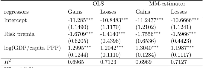
Table 1: Dependent variable: control of corruption. Cross-country, 2013.
OLS MM-estimator
regressors Gains Losses Gains Losses Intercept -11.285∗∗∗
-10.8483∗∗∗
-11.2477∗∗∗
-10.6666∗∗∗
(1.1490) (1.1170) (1.2102) (1.1241) Risk premia -1.6709∗∗∗
-1.4140∗∗∗
-1.7556∗∗∗
-1.5966∗∗∗
(0.6205) (0.4396) (0.6536) (0.4423) log(GDP/capita PPP) 1.2995∗∗∗
1.2042∗∗∗
1.3040∗∗∗
1.1987∗∗∗
(0.1244) (0.1110) (0.1284) (0.1117)
R2 0.6965 0.7123 0.6969 0.7127
∗∗∗
p <0.01
in office, the politician may react to economic developments by adjusting his level of corruption.
3
Risk aversion and corruption
In the previous section, we showed that higher agents’ risk aversion should lead to a higher tolerance of corruption. In this section we check if this assertion can be observed empirically.
Rieger et al. (2014) performed experiments in 53 countries around the world to estimate risk premia that agents require for uncertain outcomes. Agents were given a number of lotteries, with a certain probability of success and asked about what price they would pay to participate in such a lottery. The difference between the expected value of the lottery and the average price agents were willing to pay for a lottery gives an estimate of the risk premia. So that results were independent of currencies, the authors divided them by the expected value of the lottery premia.
of GDP per capita PPP, which reflects the level of the countries’ economic de-velopment. We present OLS estimates, and check robustness using a robust MM-estimator. The results are very similar. A higher risk premia corresponds to a lower control of corruption and all the estimates are statistically significant at the 0.01 significance level. This result is in line with our theoretical model; however, the resulting estimates may suffer from various endogeneity problems. For example, both risk premia and control of corruption may be affected by country-specific historical development, culture and traditions. Unfortunately, the existing data on risk aversion does not offer a solution to these problems. Nevertheless, in the next section, we assess the predictions of our model us-ing fixed-effects panel model techniques, which solve the endogeneity problems resulting from the time-invariant omitted variables.
4
Economic growth and corruption
In this section, we present a number of empirical models to verify whether adjustments to the level of corruption as a response to changes in economic development takes place in practice.
4.1
Data and preliminary analysis
We analyse the data of CIS countries; namely: Armenia, Azerbaijan, Belarus, Kazakhstan, Kyrgyzstan, Moldova, Russia, Tajikistan, Uzbekistan. Georgia, Ukraine and Turkmenistan are not considered as CIS countries, because Ukraine and Turkmenistan have never been full members, and Georgia withdrew in 2008. We analyse the CIS countries because the corruption level in these countries is high enough to give corrupt politicians some space to adjust the level of corruption in response to economic shocks. The data range is 2002-2016. The range of explanatory variables, taken with lags, was extended to 2000-2016.
Our main variables of interest are the control of corruption and GDP growth in constant 2010 prices. We also control for a number of factors - common control variables in the literature: the size of the state measured as government revenue as percentage of GDP, rule of law, voice and accountability, regulatory quality.3
We combined data from several sources. Control of corruption, rule of law, voice & accountability and regulatory quality were taken from the World Bank (W.B.) Worldwide Governance Indicators. GDP growth was calculated from the GDP per capita in 2010 prices, obtained from the W.B. World Development Indicators. Government revenue as a percentage of GDP was obtained from the IMF World Economic Outlook Database, (April 2018). Table 2 presents descriptive statistics of these variables. In Appendix 3, their correlation matrix is presented.
By definition, control of corruption “reflects perceptions of the extent to which public power is exercised for private gain, including both petty and grand forms of corruption, as well as “capture” of the state by elites and private
3
Table 2: Descriptive statistics
regressors Mean S. D. Min Max Source
Control of corruption -0.9452 0.2495 -1.37 -0.29 WB Worldwide Governance Indicators GDP/capita growth 6.2364 5.4875 -14.15 34.50 WB World Development Indicators Gov. income %GDP 30.8072 8.2593 13.60 50.76 IMF World Economic Outlook Database Rule of law -0.8300 0.3670 -1.48 -0.11 WB Worldwide Governance Indicators Voice & Account. -1.0965 0.5245 -2.12 0.05 WB Worldwide Governance Indicators Regulatory Quality -0.7017 0.4750 -1.71 0.02 WB Worldwide Governance Indicators
interests”. It takes values in the [-2.5, 2.5] interval, higher values corresponding to a better control of corruption. Rule of law, Voice & Accountability and Regulatory Quality take values in the same range, higher values reflecting better performance.
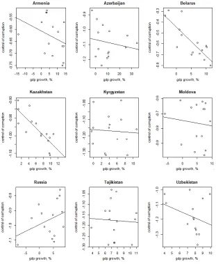
Figure 1 presents some preliminary analysis of the dependence between eco-nomic growth and corruption in the countries under analysis. In all countries except Russia, there is a negative correlation between these two factors: local authorities reduce corruption as a response to lower economic growth, and in-crease it during the periods of economic growth. In Kyrgyzstan, Moldova and Tajikistan this correlation is rather weak, but in Belarus and Kazakhstan the negative dependence is strong. Such behaviour is in line with the predictions of our theoretical model. On the contrary, in Russia, the correlation between GDP growth and control of corruption is positive. Perhaps Russian authorities rely upon other methods to remain in office during periods of economic decline. Further, a more detailed analysis is implemented.
4.2
Results
In practice, the actions of corrupt governments are not implemented immedi-ately after a crisis starts. The governments first need to understand that the crisis has taken a place. Second, they need to consider possible measures to remain in office, taking different scenarios into account. When a decision is reached, central authorities must signal officials at the lower levels. Therefore, considering the regression of control of corruption on economic growth, it is more logical to take economic growth with a lag. We include economic growth with a one and two year lag.
4.2.1 Static panel models
We regress control of corruption on GDP per capita growth, taken with one and two year lags, and other control variables. Fixed country-specific and time effects are used. The model has the following analytical expression:
CoCc,t =fc+ft+a′Xc,t+ǫc,t, (10)
where index c - denotes a country, t- time, CoCc,t- control of corruption, fc
- fixed country effect, ft - fixed time effects, Xc,t - a matrix of explanatory
Figure 1: GDP growth vs. control of corruption in CIS countries
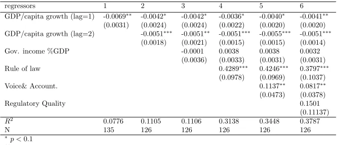
Table 3: Dependent variable: Control of corruption: Static panel, fixed individ-ual and time effects
regressors 1 2 3 4 5 6
GDP/capita growth (lag=1) -0.0069∗∗
-0.0042∗
-0.0042∗
-0.0036∗
-0.0040∗
-0.0041∗∗ (0.0031) (0.0024) (0.0024) (0.0022) (0.0020) (0.0020) GDP/capita growth (lag=2) -0.0051∗∗∗
-0.0051∗∗
-0.0051∗∗∗
-0.0055∗∗∗
-0.0051∗∗∗ (0.0018) (0.0021) (0.0015) (0.0015) (0.0014)
Gov. income %GDP -0.0001 0.0038 0.0038 0.0032
(0.0036) (0.0033) (0.0031) (0.0031)
Rule of law 0.4289∗∗∗
0.4246∗∗∗
0.3797∗∗∗ (0.0978) (0.0969) (0.1037)
Voice& Account. 0.1137∗∗
0.0817∗∗ (0.0473) (0.0378)
Regulatory Quality 0.1501
(0.11137)
R2 0.0776 0.1105 0.1106 0.3138 0.3448 0.3787
N 135 126 126 126 126 126
∗
p <0.1 ∗∗
p <0.05 ∗∗∗
p <0.01 significance level
parameters,ǫc,t - residuals of the model. The inclusion of country-fixed effects
solves many endogeneity problems, which result from time-invariant economic factors, not considered in our model, i.e., diverse history, culture and mentality. Table 3 presents estimates of a static panel model. The robust standard Arel-lano type errors (ArelArel-lano 1987) are presented in parentheses, as the residuals are autocorrelated.4 The use of Arellano-type standard errors also takes
possi-ble heteroscedasticity into account. The Shapiro-Wilk normality test (Shapiro and Wilk 1965) does not reject the hypothesis that the residuals are normal. The corresponding p-values are in the range: [0.5995-0.8746].
We include one and two years lags of economic growth and gradually add other control variables into the model. These factors are included in the model with no lags.
In all models, GDP per capita growth with one-year lag is negative and significant at the 10% significance level. The coefficient of the second year lag is also negative and larger in absolute size compared to the one-year lag; its standard deviation is lower, resulting in a very high statistical significance. This negative relation between control of corruption and economic growth is in line with our theoretical predictions. However, the quantitative impact is moderate. For example, if in 2014 and 2015 economic growth in Belarus had been 5% higher, its world rank in the control of corruption index would have declined from 108 to 115 in 2016. The other two factors which make a statistically significant impact are the rule of law (1% significance level) and voice and accountability (5% significance level). Both variables have positive coefficients, implying that the vigorous rule of law, and a higher level of democracy are associated with better control of corruption. Government income as a percentage of GDP and
4
Wooldridge’s test for serial correlation results in p-values in the range [2.2·10−
16
−9.2·
10−10] (Wooldridge 2010, pp. 310-312); the p-values corresponding to the Breusch-Godfrey test (Breusch 1978; Godfrey 1978) are in the range [5.612·10−
8
−1.026·10− 3
regulatory quality make no statistically significant impact.
Despite controling for a number of factors, our models can still carry a num-ber of endogeneity problems. For example, reduced control of corruption may suppress GDP growth; a number of studies analysed this reverse link in detail (see Mauro (1995), Ehrlich and Lui (1999) and Mo (2001), for example). Using GDP growth with lags allows us to consider Granger causality. However, we recognize that we cannot solve this endogeneity problem completely. Neverthe-less, it is possible to note that the reverse link, implies a positive dependence between the growth of GDP per capita and control of corruption. Therefore, our estimates of the coefficients are likely to be biased upwards, and the nega-tive link between economic growth and control of corruption is underestimated. Similarly, there can be a bilateral dependence between the control of corruption and the rule of law, and/or other explanatory variables. In general, such a re-verse causality may affect our estimates for economic growth. Nevertheless, the gradual inclusion of the control variables does not cause an essential change in our estimates or in their significance. This implies that our results are robust to these endogeneity problems.
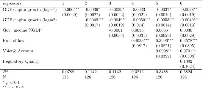
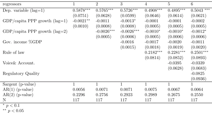
As the values of control of corruption are limited by the interval [-2.5, 2.5], it is logical to consider their transformation similar to the logit. In Appendix 4, we present estimates for the models with transformed dependent variables, using such a transformation. The results are very similar to those presented in table 3. Furthermore, as an additional robustness check, in Appendix 5, we also present estimates with an alternative measure of GDP growth. Instead of using GDP growth in constant prices, we used the growth of GDP PPP in constant prices. The results are very similar, though the coefficient corresponding to the regulatory quality became significant at the 5% significance level.
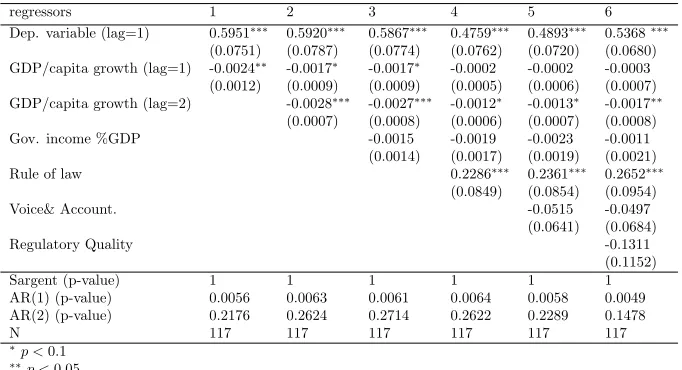
4.2.2 Dynamic panel models
In a recent work, Engler (2016) argued that agents get used to certain levels of corruption, and their satisfaction is affected not by the level of corruption itself, but by deviations from its previous levels. In order to take these findings into account, we add dynamic terms of the endogenous variable into the model. Its functional form becomes
CoCc,t=αCoCc,t−1+fc+b
′
Xc,t+εc,t, (11)
whereαis a parameter,b- a vector of parameters,εc,t - residuals of the model.
We do not include time-fixed effects, because they result in singularity problems. In all models, we used six lags of the dependent variable as instruments.
Table 4: Dependent variable: Control of corruption: Dynamic panel, fixed individual effects
regressors 1 2 3 4 5 6
Dep. variable (lag=1) 0.5951∗∗∗
0.5920∗∗∗
0.5867∗∗∗
0.4759∗∗∗
0.4893∗∗∗
0.5368∗∗∗
(0.0751) (0.0787) (0.0774) (0.0762) (0.0720) (0.0680) GDP/capita growth (lag=1) -0.0024∗∗
-0.0017∗
-0.0017∗
-0.0002 -0.0002 -0.0003 (0.0012) (0.0009) (0.0009) (0.0005) (0.0006) (0.0007) GDP/capita growth (lag=2) -0.0028∗∗∗
-0.0027∗∗∗
-0.0012∗
-0.0013∗
-0.0017∗∗
(0.0007) (0.0008) (0.0006) (0.0007) (0.0008) Gov. income %GDP -0.0015 -0.0019 -0.0023 -0.0011
(0.0014) (0.0017) (0.0019) (0.0021) Rule of law 0.2286∗∗∗
0.2361∗∗∗
0.2652∗∗∗
(0.0849) (0.0854) (0.0954) Voice& Account. -0.0515 -0.0497
(0.0641) (0.0684)
Regulatory Quality -0.1311
(0.1152) Sargent (p-value) 1 1 1 1 1 1 AR(1) (p-value) 0.0056 0.0063 0.0061 0.0064 0.0058 0.0049 AR(2) (p-value) 0.2176 0.2624 0.2714 0.2622 0.2289 0.1478
N 117 117 117 117 117 117
∗
p <0.1
∗∗
p <0.05
∗∗∗
p <0.01 significance level
per capita with a one year lag sharply declines in the absolute size and loses its significance, but the negative sign remains. Moreover, inclusion of the rule of law reduces the absolute size of the coefficient corresponding to the two-year lag of GDP growth. These estimates, combined with a negative correlation between GDP growth and the rule of law (see Appendix 3), imply that a decline in GDP growth motivates governments to strengthen the rule of law, thus affecting the control of corruption. This indirect effect of economic growth on the control of corruption accounts for a large portion of the total effect.
The control of corruption at timet−1, has a positive and highly significant impact on the control of corruption at timet. The coefficients corresponding to the rule of law remained positive and highly significant as in the static model; however, voice and accountability became insignificant. The coefficients corre-sponding to other control variables were also insignificant.
The Arellano-Bond statistics AR(1) and AR(2) (Arellano and Bond 1991) show that the errors in the first difference regression exhibit first order cor-relation (it should be so due to the lagged dependent variable in the model), but there is no second-order correlation. This indicates that the instruments are selected properly. However, the Shapiro-Wilk normality test rejects the hypoth-esis of the normality of residuals at the 5% significance level in models 1, 4, 5 and 6; the corresponding p-values are in the [0.0255, 0.0409] interval. Although the t-test is rather robust, standard errors of the coefficients may be slightly underestimated in these models.
Therefore, we can conclude that the empirical data on CIS countries are in line with the theoretical predictions of our model; however, corruption adjusts to economic development with a 1-2 year delay.
5
Conclusions
In this paper, we developed a model which shows that corrupt politicians have few incentives to implement unpopular reforms. Consequently, agents who pre-fer the status quo have incentives to tolerate corruption. Even a low proba-bility of unsuccessful reforms results in tolerance of corruption if the agents’ risk aversion is high enough. Similarly, great future benefits of reforms, may not compensate short-run losses if the elasticity of intertemporal substitution is low. In such cases, agents prefer stability even if it implies some losses due to corruption.
In contrast to models with no corruption, which predict that the politician in office shall be replaced during the periods of economic hardship, our model allows for corrupt politicians to remain in office. In this case, corrupt politicians can mitigate agents’ losses due to economic decline by reducing the amount they steal. The predicted negative relation between control of corruption and economic growth was revealed empirically in the CIS countries for the 2002-2016 period, but changes in the control of corruption follow with a 1-2 year delay.
Our model also predicts that if a corrupt politician in office behaves op-timally, he may fall from power during a serious crisis. The extent of such a crisis depends on the voters’ risk aversion and the elasticity of intertempo-ral substitution. The more risk averse the voters and the lower the elasticity of intertemporal substitution, the less likely it is that the politician in office changes.
One indirect consequence of our analysis is that policymakers who wish to implement a new reform, should take agents’ risk aversion into account. It is essential to explain the short and long-run effects of reforms, so that agents might better understand their mechanisms and so that their effects would seem more deterministic from the agents’ point of view. Limiting uncertainty, would go a long way to increase agents’ tolerance of reforms. Failure to do so, may create an oppening for corrupt populists to take office, with the likelihood that they will remain in office for a long time.
Conflict of interest
Acknowledgements
I would like to thank Leonid Polishchuk for discussions during the early version of this paper. I am also grateful to Yury Pleskachev and Aleksandr Tomaev for help with finding relevant literature, and to Georgy Idrisov for general discus-sion.
References
Arellano, M. (1987). Computing robust standard errors for within-groups estimators.Oxford Bulletin of Economics and Statistics 49(4), 431–34. Arellano, M. and S. Bond (1991). Some tests of specification for panel data:
Monte Carlo evidence and an application to employment equations.The Review of Economic Studies 58(2), 277–297.
Besley, T. and A. Prat (2006). Handcuffs for the grabbing hand? Media cap-ture and government accountability. American Economic Review 96(3), 720–736.
Boeri, T., A. B¨orsch-Supan, and G. Tabellini (2002). Pension reforms and the opinions of European citizens. American Economic Review 92(2), 396– 401.
Breusch, T. S. (1978). Testing for autocorrelation in dynamic linear models.
Australian Economic Papers 17(31), 334–355.
Breyer, F. (1989). On the intergenerational Pareto efficiency of pay-as-you-go financed pension systems. Journal of Institutional and Theoretical Eco-nomics (JITE)/Zeitschrift f¨ur die gesamte Staatswissenschaft, 643–658. Brooks, C. and J. Manza (2006). Why do welfare states persist? Journal of
Politics 68(4), 816–827.
Bucciol, A., L. Cavalli, I. Fedotenkov, P. Pertile, V. Polin, N. Sartor, and A. Sommacal (2017). A large scale OLG model for the analysis of the re-distributive effects of policy reforms.European Journal of Political Econ-omy 48, 104–127.
Charron, N. and A. B˚agenholm (2016). Ideology, party systems and corrup-tion voting in European democracies.Electoral Studies 41, 35–49. Choi, E. and J. Woo (2010). Political corruption, economic performance,
and electoral outcomes: A cross-national analysis. Contemporary Poli-tics 16(3), 249–262.
Chowdhury, S. K. (2004). The effect of democracy and press freedom on corruption: An empirical test.Economics Letters 85(1), 93–101.
Cordero, G. and A. Blais (2017). Is a corrupt government totally unaccept-able? West European Politics 40(4), 645–662.
De Vries, C. E. and H. Solaz (2017). The electoral consequences of corruption.
Del Monte, A. and E. Papagni (2001). Public expenditure, corruption, and economic growth: The case of Italy.European Journal of Political Econ-omy 17(1), 1–16.
Denisova, I., M. Eller, and E. Zhuravskaya (2010). What do Russians think about transition? Economics of Transition 18(2), 249–280.
Ehrlich, I. and F. T. Lui (1999). Bureaucratic corruption and endogenous economic growth.Journal of Political Economy 107(S6), S270–S293. Engler, S. (2016). Corruption and electoral support for new political parties
in central and eastern Europe.West European Politics 39(2), 278–304. Epstein, L. and S. Zin (1989). Substitution, risk aversion, and the
tempo-ral behavior of consumption and asset returns: A theoretical framework.
Econometrica 57, 937–969.
Epstein, L. G. and S. E. Zin (1991). Substitution, risk aversion, and the tem-poral behavior of consumption and asset returns: An empirical analysis.
Journal of Political Economy 99(2), 263–286.
Fedotenkov, I. (2018). Optimal asymmetric sector-specific labour taxation in an overlapping generations model.Journal of Economics, Forthcoming. Fehr, H. and F. Kindermann (2015). Taxing capital along the transition
-not a bad idea after all? Journal of Economic Dynamics and Control 51, 64–77.
Godfrey, L. G. (1978). Testing against general autoregressive and moving av-erage error models when the regressors include lagged dependent variables.
Econometrica 46, 1293–1301.
Goldsmith, A. A. (1999). Slapping the grasping hand. American Journal of Economics and Sociology 58(4), 865–883.
Hellman, J. S. (1998). Winners take all: The politics of partial reform in postcommunist transitions.World Politics 50(2), 203–234.
Hibbs Jr, D. A. (1979). The mass public and macroeconomic performance: The dynamics of public opinion toward unemployment and inflation.
American Journal of Political Science 23, 705–731.
Hollanders, D. and B. Vis (2013). Voters’ commitment problem and reforms in welfare programs.Public Choice 155, 433–448.
Konstantinidis, I. and G. Xezonakis (2013). Sources of tolerance towards cor-rupted politicians in Greece: The role of trade offs and individual benefits.
Crime, Law and Social Change 60(5), 549–563.
Kurer, O. (2002). Why do voters support corrupt politicians? InThe Political Economy of Corruption, pp. 75–98. Routledge.
Lewis-Beck, M. S. and M. Stegmaier (2000). Economic determinants of elec-toral outcomes.Annual Review of Political Science 3(1), 183–219. Manzetti, L. and C. J. Wilson (2007). Why do corrupt governments maintain
Mauro, P. (1995). Corruption and growth. The Quarterly Journal of Eco-nomics 110(3), 681–712.
Mo, P. H. (2001). Corruption and economic growth. Journal of Comparative Economics 29(1), 66–79.
Moran, J. (2001). Democratic transitions and forms of corruption. Crime, Law and Social Change 36(4), 379–393.
Mu˜noz, J., E. Anduiza, and A. Gallego (2016). Why do voters forgive corrupt mayors? Implicit exchange, credibility of information and clean alterna-tives.Local Government Studies 42(4), 598–615.
Pereira, C. and M. A. Melo (2015). Reelecting corrupt incumbents in exchange for public goods: Rouba mas faz in Brazil.Latin American Research Re-view 50(4), 88–115.
Peterman, W. B. (2013). Determining the motives for a positive optimal tax on capital.Journal of Economic Dynamics and Control 37(1), 265–295. Rieger, M. O., M. Wang, and T. Hens (2014). Risk preferences around the
world.Management Science 61(3), 637–648.
Rose-Ackerman, S. (2007). International handbook on the economics of cor-ruption. Edward Elgar Publishing.
Sarkar, S. and G. R. Zodrow (1993). Transitional issues in moving to a direct consumption tax.National Tax Journal 46(3), 359–376.
Schleiter, P. and A. M. Voznaya (2014). Party system competitiveness and corruption.Party Politics 20(5), 675–686.
Shapiro, S. S. and M. B. Wilk (1965). An analysis of variance test for nor-mality (complete samples).Biometrika 52(3/4), 591–611.
Singer, M. M. (2013). The global economic crisis and domestic political agen-das.Electoral Studies 32(3), 404–410.
Sung, H.-E. (2004). Democracy and political corruption: A cross-national comparison.Crime, Law and Social Change 41(2), 179–193.
Van Groezen, B., H. Kiiver, and B. Unger (2009). Explaining Europeans’ preferences for pension provision. European Journal of Political Econ-omy 25(2), 237–246.
Vis, B. (2009). Governments and unpopular social policy reform: Biting the bullet or steering clear? European Journal of Political Research 48(1), 31–57.
Winters, M. S. and R. Weitz-Shapiro (2013). Lacking information or condon-ing corruption: When do voters support corrupt politicians? Comparative Politics 45(4), 418–436.
Zechmeister, E. J. and D. Zizumbo-Colunga (2013). The varying political toll of concerns about corruption in good versus bad economic times. Com-parative Political Studies 46(10), 1190–1218.
Appendix 1
Proof. Differentiate g(s) with respect tos:
∂g(s)
∂s =
v′
(w+s+r)v(w+s)−v(w+s+r)v′
(w+s)
v(w+s)2 (12)
Derivative ∂g(s)/∂s is negative when v′
(w+s+r)v(w+s)−v(w+s+
r)v′
(w+s)<0. This is the case, when ψ(s) =v′
(w+s+r)/v(w+s+r) is a decreasing function ofs.
∂ψ(s)
∂s =
v′′
(w+s+r)v(w+s)−v′
(w+s+r)2
v(w+s+r)2 (13)
As functionv(·) is concave,v′′
(w+s+r)<0, furthermore,v(w+s)>0 for
w+s >0, therefore,∂ψ(s)/∂s <0. This implies that ∂g(s)/∂s <0.
Appendix 2
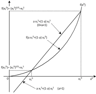
Proof. First, consider a function of the following form:
g(D) = axD1 + (1−a)x
D
2
DS (14)
wherea, x1, x2>0 andS > D. Define a functionf(x) :=xSD. This function is
strictly concave. Therefore, according to Jensen’s inequality:
g(D)< af(xD1) + (1−a)f(x2D) =axS1 + (1−a)xS2, 0< a <1. (15)
and
g(D)> af(xD1) + (1−a)f(x
D
2) =ax
S
1 + (1−a)x
S
2, a >1. (16)
These inequalities are visualised in Figure 2 in case 0 < D < S. Raising inequalities (15) and (16) into the power 1/S, we get
axD
1 + (1−a)xD2
D1 < axS
1 + (1−a)xS2
1S, 0< a <1. (17)
and
axD
1 + (1−a)xD2
D1 > axS
1 + (1−a)xS2
S1, a >1. (18)
Therefore, if 0< a <1, function g(D) is strictly increasing in D, and if a >1, functiong(D) is strictly decreasing inD. Returning to equation (8), the effects of αon φ(·) corresponds to the case 0 < a < 1, with a =p. The effect ofρ
can be seen, if 1
1−β in the denominator of the right hand side of equation (8) is
multiplied by 1ρ, witha= 1
Appendix 3
Table 5: Correlation matrix
regressors [1] [2] [3] [4] [5] [6]
[1] Control of corruption 1
[2] GDP/capita growth -0.2093 1
[3] Gov. income % GDP 0.0625 -0.1693 1
[4] Rule of law 0.4670 -0.0678 -0.1164 1
[5] Voice& Account. 0.3194 -0.1098 -0.1733 0.5907 1
[6] Regulatory Quality 0.0893 -0.1534 -0.0486 0.6116 0.7297 1
Appendix 4
In this appendix we present a static panel model with individual time and fixed effects when the control of corruption is transformed using a transformation similar to the logit:
Y = log
CoC+ 2.5 2.5−CoC
. (19)
Table 6: Dependent variable: transformed control of corruption. Static panel, fixed individual and time effects
regressors 1 2 3 4 5 6
GDP/capita growth (lag=1) -0.0065∗∗
-0.0039∗
-0.0039∗
-0.0033 -0.0037∗
-0.0038∗∗ (0.0029) (0.0022) (0.0022) (0.0021) (0.0019) (0.0019) GDP/capita growth (lag=2) -0.0049∗∗∗
-0.0049∗∗
-0.0050∗∗∗
-0.0053∗∗∗
-0.0049∗∗∗ (0.0017) (0.0019) (0.014) (0.0014) (0.0013)
Gov. income %GDP -0.0001 0.0035 0.0035 0.0030
(0.0033) (0.0031) (0.0029) (0.0029)
Rule of law 0.4033∗∗∗
0.3996∗∗∗
0.3578∗∗∗ (0.0817) (0.0821) (0.0895)
Voice& Account. 0.0998∗∗
0.0701∗∗ (0.0399) (0.0308)
Regulatory Quality 0.1392
(0.1024)
R2 0.0788 0.1142 0.1142 0.3212 0.3488 0.3824
N 135 126 126 126 126 126
∗
p <0.1 ∗∗
p <0.05 ∗∗∗
p <0.01 significance level
Appendix 5
[image:23.612.136.477.412.561.2]Table 7: Dependent variable: Control of corruption. Static panel, fixed individ-ual and time effects
regressors 1 2 3 4 5 6
GDP/capita PPP growth (lag=1) -0.0071∗∗
-0.0050∗∗
-0.0051∗∗ -0.0043∗
-0.0045∗∗
-0.0042∗∗ (0.0030) (0.0025) (0.0025) (0.0022) (0.0021) (0.0018) GDP/capita PPP growth (lag=2) -0.0045∗∗∗
-0.0045∗∗
-0.0041∗∗∗
-0.0045∗∗∗
-0.0040∗∗∗ (0.0016) (0.0020) (0.0016) (0.0017) (0.0014)
Gov. income %GDP -0.0003 0.0038 0.0034 0.0028
(0.0036) (0.0033) (0.0032) (0.0031)
Rule of law 0.4444∗∗∗
0.4432∗∗∗
0.3466∗∗∗ (0.0891) (0.0894) (0.1091)
Voice& Account. 0.1079∗∗
0.0659∗∗∗ (0.0478) (0.0187)
Regulatory Quality 0.2645∗∗∗
(0.0737)
R2 0.0798 0.1056 0.1057 0.3345 0.3634 0.4515
N 135 135 135 135 135 135
∗
p <0.1 ∗∗
p <0.05 ∗∗∗
p <0.01 significance level
Table 8: Dependent variable: Control of corruption. Dynamic panel, fixed individual effects
regressors 1 2 3 4 5 6
Dep. variable (lag=1) 0.5878∗∗∗
0.5765∗∗∗
0.5726∗∗∗
0.4908∗∗∗
0.4895∗∗∗
0.5043∗∗∗ (0.0751) (0.0628) (0.0599) (0.0646) (0.0614) (0.0621) GDP/capita PPP growth (lag=1) -0.0021∗∗
-0.0011 -0.0013∗
-0.0001 -0.0001 -0.0002 (0.0010) (0.0008) (0.0008) (0.0005) (0.0005) (0.0005) GDP/capita PPP growth (lag=2) -0.0026∗∗∗
-0.0026∗∗∗ -0.0010∗
-0.0010∗
-0.0012∗ (0.0005) (0.0006) (0.0005) (0.0006) (0.0006)
Gov. income %GDP -0.0016 -0.0017 -0.0020 -0.0011
(0.0015) (0.0018) (0.0019) (0.0020)
Rule of law 0.2182∗∗∗
0.2281∗∗∗
0.2501∗∗∗ (0.0814) (0.0852) (0.0893)
Voice& Account. -0.0395 -0.0339
(0.0628) (0.0683)
Regulatory Quality -0.0825
(0.0936)
Sargent (p-value) 1 1 1 1 1 1
AR(1) (p-value) 0.0056 0.0071 0.0071 0.0075 0.0067 0.0064
AR(2) (p-value) 0.2296 0.2756 0.2923 0.2989 0.2675 0.2550
N 117 117 117 117 117 117
∗
p <0.1 ∗∗
p <0.05 ∗∗∗
[image:24.612.136.474.359.539.2]