Improved Semantic Representations From Tree Structured Long Short Term Memory Networks

Improved Semantic Representations From

Tree-Structured Long Short-Term Memory Networks

Kai Sheng Tai, Richard Socher*, Christopher D. Manning Computer Science Department, Stanford University, *MetaMind Inc.

[email protected], [email protected], [email protected]

Abstract

Because of their superior ability to pre-serve sequence information over time, Long Short-Term Memory (LSTM) works, a type of recurrent neural net-work with a more complex computational unit, have obtained strong results on a va-riety of sequence modeling tasks. The only underlying LSTM structure that has been explored so far is a linear chain. However, natural language exhibits syn-tactic properties that would naturally com-bine words to phrases. We introduce the Tree-LSTM, a generalization of LSTMs to tree-structured network topologies. Tree-LSTMs outperform all existing systems and strong LSTM baselines on two tasks: predicting the semantic relatedness of two sentences (SemEval 2014, Task 1) and sentiment classification (Stanford Senti-ment Treebank).

1 Introduction

Most models for distributed representations of phrases and sentences—that is, models where real-valued vectors are used to represent meaning—fall into one of three classes: bag-of-words models, sequence models, and tree-structured models. In bag-of-words models, phrase and sentence repre-sentations are independent of word order; for ex-ample, they can be generated by averaging con-stituent word representations (Landauer and Du-mais, 1997; Foltz et al., 1998). In contrast, se-quence models construct sentence representations as an order-sensitive function of the sequence of tokens (Elman, 1990; Mikolov, 2012). Lastly, tree-structured models compose each phrase and sentence representation from its constituent sub-phrases according to a given syntactic structure over the sentence (Goller and Kuchler, 1996; Socher et al., 2011).

x1 x2 x3 x4

y1 y2 y3 y4

x1

x2

x4 x5 x6

y1

y2 y3

y4 y6

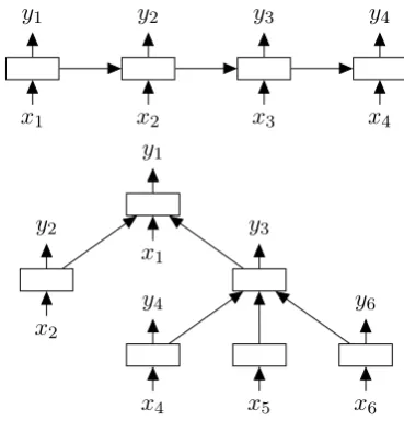
Figure 1: Top: A chain-structured LSTM net-work. Bottom: A tree-structured LSTM network with arbitrary branching factor.

Order-insensitive models are insufficient to fully capture the semantics of natural language due to their inability to account for differences in meaning as a result of differences in word order or syntactic structure (e.g., “cats climb trees” vs.

“trees climb cats”). We therefore turn to order-sensitive sequential or tree-structured models. In particular, tree-structured models are a linguisti-cally attractive option due to their relation to syn-tactic interpretations of sentence structure. A nat-ural question, then, is the following: to what ex-tent (if at all) can we do better with tree-structured models as opposed to sequential models for sen-tence representation? In this paper, we work to-wards addressing this question by directly com-paring a type of sequential model that has recently been used to achieve state-of-the-art results in sev-eral NLP tasks against its tree-structured gensev-eral- general-ization.

Due to their capability for processing arbitrary-length sequences, recurrent neural networks

(RNNs) are a natural choice for sequence model-ing tasks. Recently, RNNs with Long Short-Term Memory (LSTM) units (Hochreiter and Schmid-huber, 1997) have re-emerged as a popular archi-tecture due to their representational power and ef-fectiveness at capturing long-term dependencies. LSTM networks, which we review in Sec. 2, have been successfully applied to a variety of sequence modeling and prediction tasks, notably machine translation (Bahdanau et al., 2015; Sutskever et al., 2014), speech recognition (Graves et al., 2013), image caption generation (Vinyals et al., 2014), and program execution (Zaremba and Sutskever, 2014).

In this paper, we introduce a generalization of the standard LSTM architecture to tree-structured network topologies and show its superiority for representing sentence meaning over a sequential LSTM. While the standard LSTM composes its hidden state from the input at the current time step and the hidden state of the LSTM unit in the previous time step, the tree-structured LSTM, or Tree-LSTM, composes its state from an input vec-tor and the hidden states of arbitrarily many child units. The standard LSTM can then be considered a special case of the Tree-LSTM where each inter-nal node has exactly one child.

In our evaluations, we demonstrate the empiri-cal strength of Tree-LSTMs as models for repre-senting sentences. We evaluate the Tree-LSTM architecture on two tasks: semantic relatedness prediction on sentence pairs and sentiment clas-sification of sentences drawn from movie reviews. Our experiments show that Tree-LSTMs outper-form existing systems and sequential LSTM base-lines on both tasks. Implementations of our mod-els and experiments are available at https:// github.com/stanfordnlp/treelstm.

2 Long Short-Term Memory Networks

2.1 Overview

Recurrent neural networks (RNNs) are able to pro-cess input sequences of arbitrary length via the re-cursive application of a transition function on a

hidden state vector ht. At each time step t, the

hidden statehtis a function of the input vectorxt

that the network receives at timetand its previous hidden stateht−1. For example, the input vectorxt

could be a vector representation of thet-th word in body of text (Elman, 1990; Mikolov, 2012). The hidden state ht ∈ Rd can be interpreted as a d

-dimensional distributed representation of the se-quence of tokens observed up to timet.

Commonly, the RNN transition function is an affine transformation followed by a pointwise non-linearity such as the hyperbolic tangent function:

ht= tanh (W xt+Uht−1+b).

Unfortunately, a problem with RNNs with transi-tion functransi-tions of this form is that during training, components of the gradient vector can grow or de-cay exponentially over long sequences (Hochre-iter, 1998; Bengio et al., 1994). This problem with

explodingorvanishing gradientsmakes it difficult for the RNN model to learn long-distance correla-tions in a sequence.

The LSTM architecture (Hochreiter and Schmidhuber, 1997) addresses this problem of learning long-term dependencies by introducing a

memory cellthat is able to preserve state over long periods of time. While numerous LSTM variants have been described, here we describe the version used by Zaremba and Sutskever (2014).

We define the LSTMunitat each time steptto be a collection of vectors inRd_{: aninput gatei}

t, a forget gateft, anoutput gateot, amemory cellct

and a hidden state ht. The entries of the gating

vectorsit,ft andotare in[0,1]. We refer todas

thememory dimensionof the LSTM.

The LSTM transition equations are the follow-ing:

it=σ

W(i)xt+U(i)ht−1+b(i)

, (1)

ft=σ

W(f)xt+U(f)ht−1+b(f)

,

ot=σ

W(o)_x

t+U(o)ht−1+b(o)

,

ut= tanh

W(u)xt+U(u)ht−1+b(u)

, ct=itut+ftct−1,

ht=ottanh(ct),

wherextis the input at the current time step,σ

can learn to represent information over multiple time scales.

2.2 Variants

Two commonly-used variants of the basic LSTM architecture are the Bidirectional LSTM and the Multilayer LSTM (also known as the stacked or

deepLSTM).

Bidirectional LSTM. A Bidirectional LSTM (Graves et al., 2013) consists of two LSTMs that are run in parallel: one on the input sequence and the other on the reverse of the input sequence. At each time step, the hidden state of the Bidirec-tional LSTM is the concatenation of the forward and backward hidden states. This setup allows the hidden state to capture both past and future infor-mation.

Multilayer LSTM. In Multilayer LSTM archi-tectures, the hidden state of an LSTM unit in layer `is used as input to the LSTM unit in layer`+1in the same time step (Graves et al., 2013; Sutskever et al., 2014; Zaremba and Sutskever, 2014). Here, the idea is to let the higher layers capture longer-term dependencies of the input sequence.

These two variants can be combined as a Multi-layer Bidirectional LSTM (Graves et al., 2013).

3 Tree-Structured LSTMs

A limitation of the LSTM architectures described in the previous section is that they only allow for strictly sequential information propagation. Here, we propose two natural extensions to the basic LSTM architecture: the Child-Sum Tree-LSTM

and theN-ary Tree-LSTM. Both variants allow for richer network topologies where each LSTM unit is able to incorporate information from multiple child units.

As in standard LSTM units, each Tree-LSTM unit (indexed by j) contains input and output gates ij and oj, a memory cell cj and hidden

state hj. The difference between the standard

LSTM unit and Tree-LSTM units is that gating vectors and memory cell updates are dependent on the states of possibly many child units. Ad-ditionally, instead of a single forget gate, the Tree-LSTM unit contains one forget gate fjk for each

child k. This allows the Tree-LSTM unit to se-lectively incorporate information from each child. For example, a Tree-LSTM model can learn to em-phasize semantic heads in a semantic relatedness

h1

c1

u1

x1

c3

c2

h3

h2

f2

f3

i1 o1

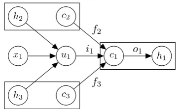
Figure 2: Composing the memory cellc1and

hid-den stateh1 of a Tree-LSTM unit with two

chil-dren (subscripts 2 and 3). Labeled edges cor-respond to gating by the indicated gating vector, with dependencies omitted for compactness.

task, or it can learn to preserve the representation of sentiment-rich children for sentiment classifica-tion.

As with the standard LSTM, each Tree-LSTM unit takes an input vectorxj. In our applications,

eachxj is a vector representation of a word in a

sentence. The input word at each node depends on the tree structure used for the network. For in-stance, in a Tree-LSTM over a dependency tree, each node in the tree takes the vector correspond-ing to the head word as input, whereas in a Tree-LSTM over a constituency tree, the leaf nodes take the corresponding word vectors as input.

3.1 Child-Sum Tree-LSTMs

Given a tree, let C(j) denote the set of children of nodej. The Child-Sum Tree-LSTM transition equations are the following:

˜

hj =

X

k∈C(j)

hk, (2)

ij =σ

W(i)_x

j+U(i)˜hj+b(i)

, (3)

fjk =σ

W(f)xj +U(f)hk+b(f)

, (4)

oj =σ

W(o)_x

j+U(o)h˜j+b(o)

, (5)

uj = tanh

W(u)xj+U(u)˜hj+b(u)

, (6) cj =ij uj +

X

k∈C(j)

fjkck, (7)

hj =ojtanh(cj), (8)

where in Eq. 4,k∈C(j).

unit, the inputxj, and the hidden stateshk of the

unit’s children. For example, in a dependency tree application, the model can learn parametersW(i)

such that the components of the input gateij have

values close to 1 (i.e., “open”) when a semanti-cally important content word (such as a verb) is given as input, and values close to 0 (i.e., “closed”) when the input is a relatively unimportant word (such as a determiner).

Dependency Tree-LSTMs. Since the Child-Sum Tree-LSTM unit conditions its components on the sum of child hidden states hk, it is

well-suited for trees with high branching factor or whose children are unordered. For example, it is a good choice for dependency trees, where the num-ber of dependents of a head can be highly variable. We refer to a Child-Sum Tree-LSTM applied to a dependency tree as aDependency Tree-LSTM.

3.2 N-ary Tree-LSTMs

TheN-ary Tree-LSTM can be used on tree struc-tures where the branching factor is at mostN and where children are ordered, i.e., they can be in-dexed from1toN. For any nodej, write the hid-den state and memory cell of itskth child ashjk

andcjkrespectively. TheN-ary Tree-LSTM

tran-sition equations are the following:

ij =σ W(i)xj+ N

X

`=1

U<sub>`</sub>(i)hj`+b(i)

! , (9)

fjk =σ W(f)xj+ N

X

`=1

U<sub>k`</sub>(f)hj`+b(f)

! ,

(10)

oj =σ W(o)xj+ N

X

`=1

U<sub>`</sub>(o)hj`+b(o)

! , (11)

uj = tanh W(u)xj+ N

X

`=1

U<sub>`</sub>(u)hj`+b(u)

! ,

(12)

cj =ijuj+ N

X

`=1

fj`cj`, (13)

hj =ojtanh(cj), (14)

where in Eq. 10, k = 1,2, . . . , N. Note that when the tree is simply a chain, both Eqs. 2–8 and Eqs. 9–14 reduce to the standard LSTM tran-sitions, Eqs. 1.

The introduction of separate parameter matri-ces for each childkallows theN-ary Tree-LSTM

model to learn more fine-grained conditioning on the states of a unit’s children than the Child-Sum Tree-LSTM. Consider, for example, a con-stituency tree application where the left child of a node corresponds to a noun phrase, and the right child to a verb phrase. Suppose that in this case it is advantageous to emphasize the verb phrase in the representation. Then the U_k`(f) parameters can be trained such that the components offj1are

close to 0 (i.e., “forget”), while the components of fj2are close to 1 (i.e., “preserve”).

Forget gate parameterization. In Eq. 10, we define a parameterization of the kth child’s for-get gate fjk that contains “off-diagonal”

param-eter matrices U<sub>k`</sub>(f), k 6= `. This parameteriza-tion allows for more flexible control of informa-tion propagainforma-tion from child to parent. For exam-ple, this allows the left hidden state in a binary tree to have either anexcitatoryorinhibitoryeffect on the forget gate of the right child. However, for large values ofN, these additional parameters are impractical and may be tied or fixed to zero.

Constituency Tree-LSTMs. We can naturally apply BinaryTree-LSTM units to binarized con-stituency trees since left and right child nodes are distinguished. We refer to this application of Bi-nary Tree-LSTMs as a Constituency Tree-LSTM. Note that in Constituency Tree-LSTMs, a nodej receives an input vectorxj only if it is a leaf node.

In the remainder of this paper, we focus on the special cases of Dependency Tree-LSTMs and Constituency Tree-LSTMs. These architectures are in fact closely related; since we consider only binarized constituency trees, the parameterizations of the two models are very similar. The key dif-ference is in the application of the compositional parameters: dependentvs. head for Dependency Tree-LSTMs, and left childvs.right child for Con-stituency Tree-LSTMs.

4 Models

We now describe two specific models that apply the Tree-LSTM architectures described in the pre-vious section.

4.1 Tree-LSTM Classification

parse tree could correspond to some property of the phrase spanned by that node.

At each node j, we use a softmax classifier to predict the labelyˆjgiven the inputs{x}j observed

at nodes in the subtree rooted atj. The classifier takes the hidden statehjat the node as input:

ˆ

pθ(y| {x}j) = softmax

W(s)_h

j+b(s)

,

ˆ

yj = arg max_y pˆθ(y| {x}j).

The cost function is the negative log-likelihood of the true class labelsy(k)_{at each labeled node:}

J(θ) =−_m1 Xm

k=1

log ˆpθ

y(k){x}(k)+λ₂kθk2₂,

where m is the number of labeled nodes in the training set, the superscriptkindicates thekth la-beled node, andλis an L2 regularization hyperpa-rameter.

4.2 Semantic Relatedness of Sentence Pairs

Given a sentence pair, we wish to predict a real-valued similarity score in some range[1, K], where K > 1 is an integer. The sequence {1,2, . . . , K} is some ordinal scale of similarity, where higher scores indicate greater degrees of similarity, and we allow real-valued scores to ac-count for ground-truth ratings that are an average over the evaluations of several human annotators.

We first produce sentence representations hL

and hR for each sentence in the pair using a

Tree-LSTM model over each sentence’s parse tree. Given these sentence representations, we predict the similarity scoreyˆusing a neural network that considers both the distance and angle between the pair(hL, hR):

h×=hLhR, (15)

h+=|hL−hR|,

hs=σ

W(×)_h

×+W(+)h++b(h)

,

ˆ

pθ = softmax

W(p)hs+b(p)

,

ˆ

y=rT_pˆ θ,

where rT _{= [1 2 . . . K]and the absolute value}

function is applied elementwise. The use of both distance measuresh× andh+ is empirically

mo-tivated: we find that the combination outperforms the use of either measure alone. The multiplicative measureh×can be interpreted as an elementwise

comparison of the signs of the input representa-tions.

We want the expected rating under the predicted distribution pˆθ given model parameters θ to be

close to the gold ratingy∈[1, K]:yˆ=rT_pˆθ≈y.

We therefore define a sparse target distribution1_p

that satisfiesy =rT_p:

pi =

    

y− byc, i=byc+ 1

byc −y+ 1, i=byc

0 otherwise

for1 ≤ i ≤ K. The cost function is the regular-ized KL-divergence betweenpandpˆθ:

J(θ) = _m1

m

X

k=1

KLp(k)pˆ(k)_θ + λ₂kθk2₂,

where m is the number of training pairs and the superscriptkindicates thekth sentence pair.

5 Experiments

We evaluate our Tree-LSTM architectures on two tasks: (1) sentiment classification of sentences sampled from movie reviews and (2) predicting the semantic relatedness of sentence pairs.

In comparing our Tree-LSTMs against sequen-tial LSTMs, we control for the number of LSTM parameters by varying the dimensionality of the hidden states2_{. Details for each model variant are}

summarized in Table 1.

5.1 Sentiment Classification

In this task, we predict the sentiment of sen-tences sampled from movie reviews. We use the Stanford Sentiment Treebank (Socher et al., 2013). There are two subtasks: binary classifica-tion of sentences, and fine-grained classificaclassifica-tion over five classes: very negative, negative, neu-tral, positive, and very positive. We use the stan-dard train/dev/test splits of 6920/872/1821 for the binary classification subtask and 8544/1101/2210 for the fine-grained classification subtask (there are fewer examples for the binary subtask since 1_{In the subsequent experiments, we found that optimizing} this objective yielded better performance than a mean squared error objective.

Relatedness Sentiment

LSTM Variant d |θ| d |θ|

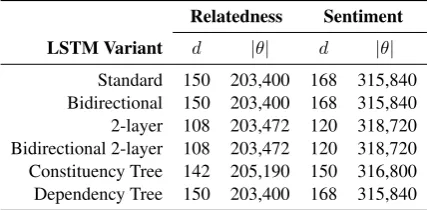
Standard 150 203,400 168 315,840 Bidirectional 150 203,400 168 315,840 2-layer 108 203,472 120 318,720 Bidirectional 2-layer 108 203,472 120 318,720 Constituency Tree 142 205,190 150 316,800 Dependency Tree 150 203,400 168 315,840

Table 1: Memory dimensions dand composition function parameter counts|θ|for each LSTM vari-ant that we evaluate.

neutral sentences are excluded). Standard bina-rized constituency parse trees are provided for each sentence in the dataset, and each node in these trees is annotated with a sentiment label.

For the sequential LSTM baselines, we predict the sentiment of a phrase using the representation given by the final LSTM hidden state. The sequen-tial LSTM models are trained on the spans corre-sponding to labeled nodes in the training set.

We use the classification model described in Sec. 4.1 with both Dependency Tree-LSTMs (Sec. 3.1) and Constituency Tree-LSTMs (Sec. 3.2). The Constituency Tree-LSTMs are structured according to the provided parse trees. For the Dependency Tree-LSTMs, we produce dependency parses3 _{of each sentence; each node}

in a tree is given a sentiment label if its span matches a labeled span in the training set.

5.2 Semantic Relatedness

For a given pair of sentences, the semantic relat-edness task is to predict a human-generated rating of the similarity of the two sentences in meaning.

We use the Sentences Involving Composi-tional Knowledge (SICK) dataset (Marelli et al., 2014), consisting of 9927 sentence pairs in a 4500/500/4927 train/dev/test split. The sentences are derived from existing image and video descrip-tion datasets. Each sentence pair is annotated with a relatedness score y ∈ [1,5], with 1 indicating that the two sentences are completely unrelated, and 5 indicating that the two sentences are very related. Each label is the average of 10 ratings as-signed by different human annotators.

Here, we use the similarity model described in Sec. 4.2. For the similarity prediction network (Eqs. 15) we use a hidden layer of size 50. We 3_{Dependency parses produced by the Stanford Neural} Network Dependency Parser (Chen and Manning, 2014).

Method Fine-grained Binary

RAE (Socher et al., 2013) 43.2 82.4 MV-RNN (Socher et al., 2013) 44.4 82.9 RNTN (Socher et al., 2013) 45.7 85.4 DCNN (Blunsom et al., 2014) 48.5 86.8 Paragraph-Vec (Le and Mikolov, 2014) 48.7 87.8 CNN-non-static (Kim, 2014) 48.0 87.2 CNN-multichannel (Kim, 2014) 47.4 88.1

DRNN (Irsoy and Cardie, 2014) 49.8 86.6

LSTM 46.4 (1.1) 84.9 (0.6)

Bidirectional LSTM 49.1 (1.0) 87.5 (0.5) 2-layer LSTM 46.0 (1.3) 86.3 (0.6) 2-layer Bidirectional LSTM 48.5 (1.0) 87.2 (1.0) Dependency Tree-LSTM 48.4 (0.4) 85.7 (0.4) Constituency Tree-LSTM

– randomly initialized vectors 43.9 (0.6) 82.0 (0.5) – Glove vectors, fixed 49.7 (0.4) 87.5 (0.8) – Glove vectors, tuned 51.0(0.5) 88.0 (0.3)

Table 2: Test set accuracies on the Stanford Sen-timent Treebank. For our experiments, we report mean accuracies over 5 runs (standard deviations in parentheses). Fine-grained: 5-class sentiment classification. Binary: positive/negative senti-ment classification.

produce binarized constituency parses4_and

depen-dency parses of the sentences in the dataset for our Constituency LSTM and Dependency Tree-LSTM models.

5.3 Hyperparameters and Training Details

The hyperparameters for our models were tuned on the development set for each task.

We initialized our word representations using publicly available 300-dimensional Glove vec-tors5 _{(Pennington et al., 2014). For the sentiment}

classification task, word representations were up-dated during training with a learning rate of 0.1. For the semantic relatedness task, word represen-tations were held fixed as we did not observe any significant improvement when the representations were tuned.

Our models were trained using AdaGrad (Duchi et al., 2011) with a learning rate of 0.05 and a minibatch size of 25. The model parameters were regularized with a per-minibatch L2 regularization strength of 10−4_{. The sentiment classifier was}

additionally regularized using dropout (Srivastava et al., 2014) with a dropout rate of 0.5. We did not observe performance gains using dropout on the semantic relatedness task.

4_{Constituency parses produced by the Stanford PCFG} Parser (Klein and Manning, 2003).

5_{Trained on 840 billion tokens of Common Crawl data,}

Method Pearson’sr Spearman’sρ MSE

Illinois-LH (Lai and Hockenmaier, 2014) 0.7993 0.7538 0.3692 UNAL-NLP (Jimenez et al., 2014) 0.8070 0.7489 0.3550 Meaning Factory (Bjerva et al., 2014) 0.8268 0.7721 0.3224

ECNU (Zhao et al., 2014) 0.8414 – –

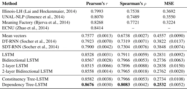
Mean vectors 0.7577 (0.0013) 0.6738 (0.0027) 0.4557 (0.0090) DT-RNN (Socher et al., 2014) 0.7923 (0.0070) 0.7319 (0.0071) 0.3822 (0.0137) SDT-RNN (Socher et al., 2014) 0.7900 (0.0042) 0.7304 (0.0076) 0.3848 (0.0074) LSTM 0.8528 (0.0031) 0.7911 (0.0059) 0.2831 (0.0092) Bidirectional LSTM 0.8567 (0.0028) 0.7966 (0.0053) 0.2736 (0.0063) 2-layer LSTM 0.8515 (0.0066) 0.7896 (0.0088) 0.2838 (0.0150) 2-layer Bidirectional LSTM 0.8558 (0.0014) 0.7965 (0.0018) 0.2762 (0.0020) Constituency Tree-LSTM 0.8582 (0.0038) 0.7966 (0.0053) 0.2734 (0.0108) Dependency Tree-LSTM 0.8676 (0.0030) 0.8083 (0.0042) 0.2532 (0.0052)

Table 3: Test set results on the SICK semantic relatedness subtask. For our experiments, we report mean scores over 5 runs (standard deviations in parentheses). Results are grouped as follows: (1) SemEval 2014 submissions;(2)Our own baselines;(3)Sequential LSTMs;(4)Tree-structured LSTMs.

6 Results

6.1 Sentiment Classification

Our results are summarized in Table 2. The Con-stituency Tree-LSTM outperforms existing sys-tems on the fine-grained classification subtask and achieves accuracy comparable to the state-of-the-art on the binary subtask. In pstate-of-the-articular, we find that it outperforms the Dependency Tree-LSTM. This performance gap is at least partially attributable to the fact that the Dependency Tree-LSTM is trained on less data: about 150K labeled nodesvs. 319K for the Constituency Tree-LSTM. This difference is due to (1) the dependency representations taining fewer nodes than the corresponding con-stituency representations, and (2) the inability to match about 9% of the dependency nodes to a cor-responding span in the training data.

We found that updating the word representa-tions during training (“fine-tuning” the word em-bedding) yields a significant boost in performance on the fine-grained classification subtask and gives a minor gain on the binary classification subtask (this finding is consistent with previous work on this task by Kim (2014)). These gains are to be expected since the Glove vectors used to initial-ize our word representations were not originally trained to capture sentiment.

6.2 Semantic Relatedness

Our results are summarized in Table 3. Following Marelli et al. (2014), we use Pearson’s r, Spear-man’sρand mean squared error (MSE) as

evalua-tion metrics. The first two metrics are measures of correlation against human evaluations of semantic relatedness.

We compare our models against a number of non-LSTM baselines. The mean vector baseline computes sentence representations as a mean of the representations of the constituent words. The DT-RNN and SDT-RNN models (Socher et al., 2014) both compose vector representations for the nodes in a dependency tree as a sum over affine-transformed child vectors, followed by a nonlin-earity. The SRNN is an extension of the DT-RNN that uses a separate transformation for each dependency relation. For each of our baselines, including the LSTM models, we use the similarity model described in Sec. 4.2.

We also compare against four of the top-performing systems6 _{submitted to the SemEval}

2014 semantic relatedness shared task: ECNU (Zhao et al., 2014), The Meaning Factory (Bjerva et al., 2014), UNAL-NLP (Jimenez et al., 2014), and Illinois-LH (Lai and Hockenmaier, 2014). These systems are heavily feature engineered, generally using a combination of surface form overlap features and lexical distance features de-rived from WordNet or the Paraphrase Database (Ganitkevitch et al., 2013).

Our LSTM models outperform all these

0 5 10 15 20 25 30 35 40 45

sentence length

0.30 0.35 0.40 0.45 0.50 0.55 0.60 0.65 0.70

accuracy

DT-LSTM CT-LSTM LSTM Bi-LSTM

Figure 3: Fine-grained sentiment classification ac-curacy vs. sentence length. For each `, we plot accuracy for the test set sentences with length in the window [`−2, `+ 2]. Examples in the tail of the length distribution are batched in the final window (`= 45).

tems without any additional feature engineering, with the best results achieved by the Dependency LSTM. Recall that in this task, both Tree-LSTM models only receive supervision at the root of the tree, in contrast to the sentiment classifi-cation task where supervision was also provided at the intermediate nodes. We conjecture that in this setting, the Dependency Tree-LSTM benefits from its more compact structure relative to the Constituency Tree-LSTM, in the sense that paths from input word vectors to the root of the tree are shorter on aggregate for the Dependency Tree-LSTM.

7 Discussion and Qualitative Analysis

7.1 Modeling Semantic Relatedness

In Table 4, we list nearest-neighbor sentences re-trieved from a 1000-sentence sample of the SICK test set. We compare the neighbors ranked by the Dependency Tree-LSTM model against a baseline ranking by cosine similarity of the mean word vec-tors for each sentence.

The Dependency Tree-LSTM model exhibits several desirable properties. Note that in the de-pendency parse of the second query sentence, the word “ocean” is the second-furthest word from the root (“waving”), with a depth of 4. Regardless, the retrieved sentences are all semantically related to the word “ocean”, which indicates that the Tree-LSTM is able to both preserve and emphasize in-formation from relatively distant nodes. Addi-tionally, the Tree-LSTM model shows greater

ro-4 6 8 10 12 14 16 18 20

mean sentence length

0.78 0.80 0.82 0.84 0.86 0.88 0.90

r

DT-LSTM CT-LSTM LSTM Bi-LSTM

Figure 4: Pearson correlations r between pre-dicted similarities and gold ratings vs. sentence length. For each `, we plot r for the pairs with mean length in the window[`−2, `+2]. Examples in the tail of the length distribution are batched in the final window (`= 18.5).

bustness to differences in sentence length. Given the query “two men are playing guitar”, the Tree-LSTM associates the phrase “playing guitar” with the longer, related phrase “dancing and singing in front of a crowd” (note as well that there is zero token overlap between the two phrases).

7.2 Effect of Sentence Length

One hypothesis to explain the empirical strength of Tree-LSTMs is that tree structures help miti-gate the problem of preserving state over long se-quences of words. If this were true, we would ex-pect to see the greatest improvement over sequen-tial LSTMs on longer sentences. In Figs. 3 and 4, we show the relationship between sentence length and performance as measured by the relevant task-specific metric. Each data point is a mean score over 5 runs, and error bars have been omitted for clarity.

We observe that while the Dependency Tree-LSTM does significantly outperform its sequen-tial counterparts on the relatedness task for longer sentences of length 13 to 15 (Fig. 4), it also achieves consistently strong performance on shorter sentences. This suggests that unlike se-quential LSTMs, Tree-LSTMs are able to encode semantically-useful structural information in the sentence representations that they compose. 8 Related Work

Ranking by mean word vector cosine similarity Score a woman is slicing potatoes

a woman is cutting potatoes 0.96

a woman is slicing herbs 0.92

a woman is slicing tofu 0.92

a boy is waving at some young runners from the ocean

a man and a boy are standing at the bottom of some stairs , 0.92 which are outdoors

a group of children in uniforms is standing at a gate and 0.90 one is kissing the mother

a group of children in uniforms is standing at a gate and 0.90 there is no one kissing the mother

two men are playing guitar

some men are playing rugby 0.88

two men are talking 0.87

two dogs are playing with each other 0.87

Ranking by Dependency Tree-LSTM model Score a woman is slicing potatoes

a woman is cutting potatoes 4.82

potatoes are being sliced by a woman 4.70 tofu is being sliced by a woman 4.39

a boy is waving at some young runners from the ocean

a group of men is playing with a ball on the beach 3.79

a young boy wearing a red swimsuit is jumping out of a 3.37 blue kiddies pool

the man is tossing a kid into the swimming pool that is 3.19 near the ocean

two men are playing guitar

the man is singing and playing the guitar 4.08 the man is opening the guitar for donations and plays 4.01

with the case

two men are dancing and singing in front of a crowd 4.00

Table 4: Most similar sentences from a 1000-sentence sample drawn from the SICK test set. The Tree-LSTM model is able to pick up on more subtle relationships, such as that between “beach” and “ocean” in the second example.

Pennington et al., 2014) have found wide appli-cability in a variety of NLP tasks. Following this success, there has been substantial interest in the area of learning distributed phrase and sen-tence representations (Mitchell and Lapata, 2010; Yessenalina and Cardie, 2011; Grefenstette et al., 2013; Mikolov et al., 2013), as well as distributed representations of longer bodies of text such as paragraphs and documents (Srivastava et al., 2013; Le and Mikolov, 2014).

Our approach builds on recursive neural net-works (Goller and Kuchler, 1996; Socher et al., 2011), which we abbreviate as Tree-RNNs in or-der to avoid confusion with recurrent neural net-works. Under the Tree-RNN framework, the vec-tor representation associated with each node of a tree is composed as a function of the vectors corresponding to the children of the node. The choice of composition function gives rise to nu-merous variants of this basic framework. Tree-RNNs have been used to parse images of natu-ral scenes (Socher et al., 2011), compose phrase representations from word vectors (Socher et al., 2012), and classify the sentiment polarity of sen-tences (Socher et al., 2013).

9 Conclusion

In this paper, we introduced a generalization of LSTMs to tree-structured network topologies. The Tree-LSTM architecture can be applied to trees with arbitrary branching factor. We demonstrated the effectiveness of the Tree-LSTM by applying the architecture in two tasks: semantic relatedness

and sentiment classification, outperforming exist-ing systems on both. Controllexist-ing for model di-mensionality, we demonstrated that Tree-LSTM models are able to outperform their sequential counterparts. Our results suggest further lines of work in characterizing the role of structure in pro-ducing distributed representations of sentences.

Acknowledgements

We thank our anonymous reviewers for their valu-able feedback. Stanford University gratefully ac-knowledges the support of a Natural Language Understanding-focused gift from Google Inc. and the Defense Advanced Research Projects Agency (DARPA) Deep Exploration and Filtering of Text (DEFT) Program under Air Force Research Lab-oratory (AFRL) contract no. FA8750-13-2-0040. Any opinions, findings, and conclusion or recom-mendations expressed in this material are those of the authors and do not necessarily reflect the view of the DARPA, AFRL, or the US government.

References

Bahdanau, Dzmitry, Kyunghyun Cho, and Yoshua Bengio. 2015. Neural machine translation by jointly learning to align and translate. In Pro-ceedings of the 3rd International Conference on Learning Representations (ICLR 2015).

Bjerva, Johannes, Johan Bos, Rob van der Goot, and Malvina Nissim. 2014. The Meaning Fac-tory: Formal semantics for recognizing textual entailment and determining semantic similarity. In Proceedings of the 8th International Work-shop on Semantic Evaluation (SemEval 2014). Blunsom, Phil, Edward Grefenstette, Nal

Kalch-brenner, et al. 2014. A convolutional neural net-work for modelling sentences. InProceedings of the 52nd Annual Meeting of the Association for Computational Linguistics.

Chen, Danqi and Christopher D Manning. 2014. A fast and accurate dependency parser using neu-ral networks. InProceedings of the 2014 Con-ference on Empirical Methods in Natural Lan-guage Processing (EMNLP).

Collobert, Ronan, Jason Weston, L´eon Bottou, Michael Karlen, Koray Kavukcuoglu, and Pavel Kuksa. 2011. Natural language processing (al-most) from scratch. The Journal of Machine Learning Research12:2493–2537.

Duchi, John, Elad Hazan, and Yoram Singer. 2011. Adaptive subgradient methods for online learn-ing and stochastic optimization. The Journal of Machine Learning Research12:2121–2159. Elman, Jeffrey L. 1990. Finding structure in time.

Cognitive science14(2):179–211.

Foltz, Peter W, Walter Kintsch, and Thomas K Landauer. 1998. The measurement of textual coherence with latent semantic analysis. Dis-course processes25(2-3):285–307.

Ganitkevitch, Juri, Benjamin Van Durme, and Chris Callison-Burch. 2013. PPDB: The Para-phrase Database. In Proceedings of HLT-NAACL 2013.

Goller, Christoph and Andreas Kuchler. 1996. Learning task-dependent distributed representa-tions by backpropagation through structure. In

IEEE International Conference on Neural Net-works.

Graves, Alex, Navdeep Jaitly, and A-R Mohamed. 2013. Hybrid speech recognition with deep bidirectional LSTM. InIEEE Workshop on Au-tomatic Speech Recognition and Understanding (ASRU).

Grefenstette, Edward, Georgiana Dinu, Yao-Zhong Zhang, Mehrnoosh Sadrzadeh, and Marco Baroni. 2013. Multi-step regression

learning for compositional distributional se-mantics. In Proceedings of the 10th Interna-tional Conference on ComputaInterna-tional Semantics. Hochreiter, Sepp. 1998. The vanishing gradient problem during learning recurrent neural nets and problem solutions.International Journal of Uncertainty, Fuzziness and Knowledge-Based Systems6(02):107–116.

Hochreiter, Sepp and J¨urgen Schmidhuber. 1997. Long Short-Term Memory. Neural Computa-tion9(8).

Huang, Eric H., Richard Socher, Christopher D. Manning, and Andrew Y. Ng. 2012. Improv-ing word representations via global context and multiple word prototypes. In Annual Meeting of the Association for Computational Linguis-tics (ACL).

Irsoy, Ozan and Claire Cardie. 2014. Deep re-cursive neural networks for compositionality in language. In Advances in Neural Information Processing Systems.

Jimenez, Sergio, George Duenas, Julia Baquero, Alexander Gelbukh, Av Juan Dios B´atiz, and Av Mendiz´abal. 2014. UNAL-NLP: Combin-ing soft cardinality features for semantic textual similarity, relatedness and entailment. In Pro-ceedings of the 8th International Workshop on Semantic Evaluation (SemEval 2014).

Kim, Yoon. 2014. Convolutional neural networks for sentence classification. In Proceedings of the 2014 Conference on Empirical Methods in Natural Language Processing (EMNLP). Klein, Dan and Christopher D Manning. 2003.

Accurate unlexicalized parsing. InProceedings of the 41st Annual Meeting on Association for Computational Linguistics.

Lai, Alice and Julia Hockenmaier. 2014. Illinois-LH: A denotational and distributional approach to semantics. In Proceedings of the 8th Inter-national Workshop on Semantic Evaluation (Se-mEval 2014).

Landauer, Thomas K and Susan T Dumais. 1997. A solution to Plato’s problem: The latent se-mantic analysis theory of acquisition, induction, and representation of knowledge.Psychological review104(2):211.

Proceedings of the 31st International Confer-ence on Machine Learning (ICML-14).

Marelli, Marco, Luisa Bentivogli, Marco Ba-roni, Raffaella Bernardi, Stefano Menini, and Roberto Zamparelli. 2014. SemEval-2014 Task 1: Evaluation of compositional distributional semantic models on full sentences through se-mantic relatedness and textual entailment. In

Proceedings of the 8th International Workshop on Semantic Evaluation (SemEval 2014). Mikolov, Tom´aˇs. 2012.Statistical Language

Mod-els Based on Neural Networks. Ph.D. thesis, Brno University of Technology.

Mikolov, Tomas, Ilya Sutskever, Kai Chen, Greg S Corrado, and Jeff Dean. 2013. Distributed representations of words and phrases and their compositionality. InAdvances in Neural Infor-mation Processing Systems.

Mitchell, Jeff and Mirella Lapata. 2010. Composi-tion in distribuComposi-tional models of semantics. Cog-nitive science34(8):1388–1429.

Pennington, Jeffrey, Richard Socher, and Christo-pher D Manning. 2014. Glove: Global vectors for word representation. InProceedings of the 2014 Conference on Empiricial Methods in Nat-ural Language Processing (EMNLP).

Rumelhart, David E, Geoffrey E Hinton, and Ronald J Williams. 1988. Learning represen-tations by back-propagating errors. Cognitive modeling5.

Socher, Richard, Brody Huval, Christopher D Manning, and Andrew Y Ng. 2012. Seman-tic compositionality through recursive matrix-vector spaces. InProceedings of the 2012 Joint Conference on Empirical Methods in Natural Language Processing and Computational Nat-ural Language Learning (EMNLP).

Socher, Richard, Andrej Karpathy, Quoc V Le, Christopher D Manning, and Andrew Y Ng. 2014. Grounded compositional semantics for finding and describing images with sentences.

Transactions of the Association for Computa-tional Linguistics2.

Socher, Richard, Cliff C Lin, Chris Manning, and Andrew Y Ng. 2011. Parsing natural scenes and natural language with recursive neural net-works. InProceedings of the 28th International Conference on Machine Learning (ICML-11).

Socher, Richard, Alex Perelygin, Jean Y Wu, Jason Chuang, Christopher D Manning, An-drew Y Ng, and Christopher Potts. 2013. Re-cursive deep models for semantic composition-ality over a sentiment treebank. InProceedings of the 2013 Conference on Empirical Methods in Natural Language Processing (EMNLP). Srivastava, Nitish, Geoffrey Hinton, Alex

Krizhevsky, Ilya Sutskever, and Ruslan Salakhutdinov. 2014. Dropout: A simple way to prevent neural networks from overfit-ting. Journal of Machine Learning Research

15:1929–1958.

Srivastava, Nitish, Ruslan Salakhutdinov, and Ge-offrey Hinton. 2013. Modeling documents with a Deep Boltzmann Machine. InUncertainty in Artificial Intelligence.

Sutskever, Ilya, Oriol Vinyals, and Quoc VV Le. 2014. Sequence to sequence learning with neu-ral networks. In Advances in Neural Informa-tion Processing Systems.

Turian, Joseph, Lev Ratinov, and Yoshua Bengio. 2010. Word representations: A simple and gen-eral method for semi-supervised learning. In

Proceedings of the 48th Annual Meeting of the Association for Computational Linguistics. Vinyals, Oriol, Alexander Toshev, Samy Bengio,

and Dumitru Erhan. 2014. Show and tell: A neural image caption generator. arXiv preprint arXiv:1411.4555.

Yessenalina, Ainur and Claire Cardie. 2011. Com-positional matrix-space models for sentiment analysis. In Proceedings of the 2011 Confer-ence on Empirical Methods in Natural Lan-guage Processing (EMNLP).

Zaremba, Wojciech and Ilya Sutskever. 2014. Learning to execute. arXiv preprint arXiv:1410.4615.