Munich Personal RePEc Archive
Eurozone Real Output and Covered
Interest Parity Deviations: Can Stronger
Real Output Lessen the Deviations?
Ibhagui, Oyakhilome
3 January 2019
Online at
https://mpra.ub.uni-muenchen.de/92305/
On the EUR/USD Cross-Currency Basis Spread: A Theory of CIP Deviations Based on the Monetary Model
Eurozone Real Output and Covered Interest Parity Deviations: Can Stronger Real Output Lessen the Deviations?
Abstract
Evidence shows that covered interest parity deviations have expanded over time in the EUR/USD cross currency basis
swap market – the world’s largest basis swap market – even across the less erratic long-end of the basis swap curve. We
analyze the long-run impact and dynamic interdependencies of eurozone macroeconomic factors on the long-end of the
EUR/USD cross-currency basis swap spread, utilizing quarterly data from 2003–2018. Our stylized model predicts that
a rise in euro area real output relative to the US would lead to a tighter euro basis swap spread; however, an increase in
euro area money supply relative to the US as well as a depreciation of the euro would widen the euro basis in the long
run. Our model suggests that the magnitude of the effect of real output on the basis is particularly more pronounced than
the magnitude of the individual or combined effect of money supply increases and euro depreciation on the basis.
Interestingly, our empirical results are consistent with these predictions. In addition, after examining convergence to long
run, we find that among the eurozone variables, it is the cross-currency basis that is the predominant adjusting variable
in the event of a divergence from the estimated long-run relation. Finally, using accumulated impulse response, we show
that shocks to the exchange rate which strengthen the US dollar have permanent effects on the basis.
Keywords: eurozone, exchange rates, money supply, real output and euro cross-currency basis
JEL Classifications: E4, E5, E6, F3, G1, G2
I. Introduction
A major shift in the global financial markets over the last decade - one which has added an important variable to the
list of carefully monitored indicators in the financial markets - is the persistent breakdown of covered interest parity
(CIP). At its core, the CIP is a no arbitrage condition. In simple terms1, it states that, given two currencies $ and €,
the income realized when a $ holder invests in a € fixed income security and exchanges the € proceeds to $ must be
equivalent to the income generated had the $ holder invested in a similar $ security domestically. This also implies
that when a euro entity issues in $ and exchanges the cost of the $ funds raised to €, this cost must be equal to that
1How a pure arbitrage profit from CIP deviations - manifested as a negative cross-currency basis between the euro and U.S. dollars – can be made. We start
by assuming the arbitrageur has no dollar in hand. To arbitrage in the euro market, the U.S. dollar arbitrageur borrows one $1 at the interest rate i and converts the $1 into euro at a rate of $1 to S euro. This gives S euro. The arbitrageur then approaches the euro zone financial market, lends out the euro at the prevailing euro market interest rate i*, and then signs a forward contract on the same date to convert the euro proceeds to the U.S dollar at a future date when the deal expires, i.e. at maturity or end of investment horizon. At maturity, which is at the end of the investment horizon n, the arbitrageur receives 𝑆𝑒𝑛𝑖∗≃ 𝑆(1 + 𝑖∗)𝑛 in euros, and converts this sum into 𝑆𝑒𝑛𝑖∗/𝐹 = 𝑆(1 + 𝑖∗)𝑛/𝐹 U.S. dollars due to the forward contract 𝐹. At the end of the
incurred had the euro entity issued a similar product domestically in €. Otherwise, it would be possible to raise
cheaper € funds via issuing in $ or obtain a higher income in $ via €, with currency risk fully hedged. The CIP
breakdown became most visible in the last crises and has since persisted – offering the possibility to access cheaper
funds or make arbitrage profits than would have been possible had the CIP remained largely unbroken. The CIP
breakdown is encoded in what has now been known as the cross-currency basis swap spread. If CIP existed, this
spread would be zero. Thus, the non-zero nature of the spread captures the magnitude or extent of CIP breakdown.
This variable also indicates the level of stress in the financial market. For the euro basis, it is highly negative across
maturities, including at the low volatility and less erratic long end of the basis curve which is the focus of this paper.
Much of the recent studies on cross-currency basis swap spreads have been skewed towards explaining why
risk-free arbitrage still exists and why the spreads have not fizzled out, what the spreads imply about the credit risk in
currencies, how they relate to the general demand for dollar-based assets and how post-crisis regulations - which
impose balance sheet constraints that limit the size of exposures that banks and non-banks can take - have impacted
the basis spreads. One of the major findings in the literature is that the CIP breakdown persists because banks, and
other financial institutions that depend on them, are constrained, by increase regulations post crisis, from exploiting
the opportunities which the CIP breakdown affords. As a result, the opportunities remain, because they have not
been fully exploited, and the euro cross-currency basis remains deeply negative across maturities. But how do
macroeconomic factors contribute to the persistence of the cross-currency basis? The role of macroeconomic factors
in the persistence of the euro cross-currency basis has remained largely ignored in the literature. Since financial
markets necessarily rely on benign macroeconomic conditions, then information on cross-currency basis swap
spreads should be contained in some macroeconomic factors. The focus of this paper, therefore, is on what we can
learn about the euro cross-currency basis swap spread from macroeconomic factors in the euro area.
Another motivation for this study is that the limited existing literature on CIP breakdown has focused almost
exclusively on the strength of the dollar exchange rate as a major mechanism responsible for driving the
cross-currency basis wider, in line with the findings by Avdjiev et al. (2017). Although this is true and is confirmed in our
study, we believe this does not tell the full story. First, whilst it is true that an increase in dollar strength could reduce
the amount of dollar flows to other countries or dollar lending activities as the fear of potential default increases as
a stronger dollar burdens the ability of borrowers or counter parties to meet obligations, which would slow
cross-border dollar flows and appetite for non-dollar assets, it is also important to note that other factors, such as a more
favorable economic performance exist that could raise cross border dollar flows even amid an increasing dollar
strength. As such, the dollar will be dominant and exert the most considerable influence on the cross-currency basis
swap spreads only when other indicators of financial and economic health are less benign. Second, an exclusive
focus on the dollar neglects the potentially substantial impact of broader economic drivers on the cross-currency
basis swap spreads, an effect already emphasized by the low coefficient of determination for the dollar as the main
driver of the basis in existing studies. We seek to address these highlighted gaps in the literature by emphasizing the
role played not only by the exchange rate but also by the real and monetary aspects of the economy in determining
To understand the impact of eurozone macroeconomic factors on the euro cross-currency basis, we construct a model
relating the euro cross-currency basis with standard macroeconomic factors – exchange rate, money supply and real
output representing relative currency prices, monetary policy and performance of the real economy, respectively.
We model the cross-currency basis as a deviation from CIP, in line with the standard definition. Our model predicts
a tightening of the euro cross-currency basis in the long run when real output increases in the eurozone relative to
the U.S., but a widening of the basis following a rise in euro area money supply and a depreciation of the euro
exchange rate. We take these predictions to a euro data set and directly investigated their implications for the euro
cross-currency basis. We do this to make sure that our theoretical results are not a mere coincidence and that they
adequately fit and are consistent with the euro data. We first examine the non-stationarity and cointegration property
of the euro data. Our results show that the macroeconomic variables and euro cross-currency basis swap are
cointegrated, implying the existence of an estimable long-run relationship in levels. To estimate the long-run
relationship, we employ appropriate estimators for cointegrated time series such as dynamic OLS, fully modified
OLS and canonical cointegrating regression.
After estimating the coefficients on the macroeconomic variables, we find that our results are consistent with the
predictions of our model in that they show an economically and statistically significant long run relationship between
macroeconomic factors in the euro area and euro cross-currency basis swap spreads. The major finding of our paper
is that the theoretical model is strongly supported by euro area data. The key message from the model and data is
that macroeconomic factors play a significant role in the behavior of the euro cross-currency basis spreads in the
long run. In particular, we find that real output, money supply and the exchange rate are linked in the long run; the
linkage is such that i) an increase in Euro area output relative to US real output tightens the euro basis, ii) an increase
in euro money supply relative to US money supply widens the basis and iii) a depreciation of the EURUSD exchange
rate also widens the basis. We find that these results are generally true across all estimators employed. Thus, in the
long-run, deviations from CIP in the eurozone turn on the strength of the dollar relative to the euro and the scale of
money supply in the Euro area. When eurozone money supply increases and the dollar strengthens relative to the
euro, deviations from CIP become larger and the euro cross-currency basis swap spreads tend to widen in the long
run.
Our point estimates across all estimators considered indicate that, other things being equal, a 1 basis-point increase in
the eurozone real output relative to the U.S tightens the 10-year euro cross-currency basis by 7.70 – 9.44 basis points per
quarter, while a 1 basis-point depreciation in the EUR/USD exchange rate and an increase in euro area broad money
supply widens the 10-year euro cross-currency basis by 1.07 – 2.98 basis points and 2.32 – 5.11 basis points, respectively.
This indicates that in the long run, most of the tightening in the long end of the euro basis is driven by an improvement
in real output in the eurozone. Not only is this important, it is able to offset the widening pressure from currency
depreciation and money supply increases as our point estimates have shown.
We also investigate the dynamic impact of the error correction term on the changes of each of the variables in the
cointegrated vector in order to get a sense of the adjustment back to equilibrium following a temporary deviation. We
of adjustment implies a half-life for cross-currency misalignments of just over 5 quarters. With respect to the
macroeconomic variables, the error correction variable has either no explanatory power for their dynamics or yields a
positive sign unsupportive of convergence. Lastly, we show that shocks to the exchange rate, which strengthen the US
dollar, have permanent effects on the basis.
We have focused on the euro area for several reasons. First, there has been a significant increase of international
bond issuance in the euro since the launch of the European monetary union, Hale and Spiegel (2012). Also, Avdjiev
et al. (2017) find evidence that the euro has started to exhibit characteristics of a global funding currency. This makes
a study examining the link between eurozone macroeconomic factors and the EUR/USD cross-currency basis very
important especially given that the euro proceeds obtained are often of intermediate importance and the final currency
of need for a large amount of these issues, especially for large multilateral development institutions, is often in a
different currency from the euro and often swapped to a different currency, mostly the US dollars. Second, euro
cross-currency basis swap market is the most active basis swap market, accounting for 46% of volumes (see Barnes
(2017)). The EUR/USD basis is the largest cross-currency swap market. Moreover, the EUR/USD is a very liquid
currency pair and is the most traded foreign exchange pair among the G10 currencies, accounting for over 20% of
the total volume of transactions in the forex market, thus providing adequate and required variability in the data for
analysis. Third, the eurozone is the largest and best known monetary union which affords the region with
macroeconomic scale and size, a broader based, synchronized monetary policy, and increases the internationalization
of the euro in global payments and foreign exchange settlements.
To provide a graphical illustration of what turns out to support our model and empirical finding, Figure 1 below plots
the cross-currency (in blue) paired with the relative real output (ash), relative money supply (purple) and exchange
rate (black) over time. A cursory look at the graphs suggest that when the ash line goes down, which means the
eurozone real output underperforms the US output, the cross-currency basis (blue line) tends to widen. We also see
that when the purple line increases, which means that the eurozone money supply increases relative to the US money
supply, the cross-currency basis tends to widen. In fact, as it can be seen, the cross-currency basis, by and large, is
often the mirror image of the relative money supply. Lastly, the plot of the EUR/USD exchange rate are shown below
in black. When the lines go up, the dollar strengthens (or the euro weakens) and when they go down, the euro
strengthens, or the dollar weakens. Again, as with money supply, we see that the euro cross-currency basis is the
mirror image of the euro weakness or dollar strength. When the euro weakens (or the dollar strengthens), the
Figure 1a: 10-year cross-currency basis paired with relative output, money supply, spot and forward exchange rate
The rest of the paper is organized as follows. Section II reports some stylized facts about the euro basis while Section
III presents the baseline model framework which forms the basis of subsequent empirical analysis. Section IV
explains the data, empirical methodology as well as the empirical result while Section V analyzes the convergence
to long run via error-correction analysis. Section VI presents the dynamic interdependencies using VAR, and Section
VII provides a comparison with other empirical studies. The last section concludes.
II. The EUR Basis – Stylized Fact
Here, we present some stylized facts on the euro cross-currency basis swap spreads. We take a cursory look at the
basis at the 3-month, 5-year and 10-year maturity buckets and across notable periods over the past decades. The
tables below summarize the quarterly behavior of the basis across the three maturities over the i) whole sample
period (2013 to 2018), ii) global financial crisis period (2007 to 2009), iii) eurozone sovereign crisis period (2010 -0.86 -0.85 -0.84 -0.83 -0.82 -0.81 -0.8 -0.79 -0.78 -0.77 -0.76 -60 -50 -40 -30 -20 -10 0 10 3/1/2003
10/1/2003 5/1/2004 12/1/2004 7/1/2005 2/1/2006 9/1/2006 4/1/2007 11/1/2007 6/1/2008 1/1/2009 8/1/2009 3/1
/20
10
10/1/2010 5/1/2011 12
/1/2
01
1
7/1/2012 2/1/2013 9/1
/20 13 4/1/2014 11/1/2014 6/1 /20 15
1/1/2016 8/1/2016 3/1/2017 10/1/2017 5/1/2018
Cross-currency basis swap spread (LHS) Eurozone-US relative real output, in logs (RHS)
-0.25 -0.2 -0.15 -0.1 -0.05 0 -60 -50 -40 -30 -20 -10 0 10
3/1/2003 6/1/2004 9/1/2005 12/1/2006 3/1
/20
08
6/1/2009 9/1/2010
12/1/2011 3/1/2013 6/1/2014 9/1/2015 12/1/2016 3/1/2018
Cross-currency basis swap spread (LHS)
EURUSD spot exchange rate, in logs
-0.1 -0.08 -0.06 -0.04 -0.02 0 0.02 -60 -50 -40 -30 -20 -10 0 10 3/1/2003 7/1/2004
11/1/2005 3/1/2007 7/1/2008 11/1/2009 3/1/2011 7/1/2012 11/1/2013 3/1/2015 7/1/2016 11/1/2017
Cross-currency basis swap spread (LHS)
to 2012), iv) combined crisis periods (2007 to 2012) and, finally, v) the period post crisis (2003 to 2018),
[image:7.612.83.568.80.540.2]respectively.
Fig 1b: Evolution of the euro cross-currency basis swap spreads
We begin with the whole sample period. In this case, across the three maturities, the 3-month euro basis is the
widest, on average, and has the highest volatility. This is followed by the 5-year euro basis while the 10-year euro
basis is the tightest and has the least volatility across the three maturities. The 3-month EUR basis seems to diverge
significantly from the 5-year and 10-year basis, both of which appear to be well synchronized. The correlation
analysis presented below confirms this observation quite well. -200 -150 -100 -50 0 50 3 /1 /2 0 0 3 1 2 /1 /2 0 0 3 9 /1 /2 0 0 4 6 /1 /2 0 0 5 3 /1 /2 0 0 6 1 2 /1 /2 0 0 6 9 /1 /2 0 0 7 6 /1 /2 0 0 8 3 /1 /2 0 0 9 1 2 /1 /2 0 0 9 9 /1 /2 0 1 0 6 /1 /2 0 1 1 3 /1 /2 0 1 2 1 2 /1 /2 0 1 2 9 /1 /2 0 1 3 6 /1 /2 0 1 4 3 /1 /2 0 1 5 1 2 /1 /2 0 1 5 9 /1 /2 0 1 6 6 /1 /2 0 1 7 3 /1 /2 0 1 8
Whole Sample Period
10Y EUR 5Y EUR 3M EUR
-60 -50 -40 -30 -20 -10 0 3/1 /201 3 8/1 /201 3 1/1 /201 4 6/1 /201 4 11/ 1/20 14 4/1 /201 5 9/1 /201 5 2/1 /201 6 7/1 /201 6 12/ 1/20 16 5/1 /201 7 10/ 1/20 17 3/1 /201 8 8/1 /201 8
Post Global and Eurozone Crises Period
10Y EUR 5Y EUR 3M EUR
-200 -180 -160 -140 -120 -100 -80 -60 -40 -20 0 1 2 /1 /2 0 0 7 1 /1 /2 0 0 8 2 /1 /2 0 0 8 3 /1 /2 0 0 8 4 /1 /2 0 0 8 5 /1 /2 0 0 8 6 /1 /2 0 0 8 7 /1 /2 0 0 8 8 /1 /2 0 0 8 9 /1 /2 0 0 8 1 0 /1 /2 0 0 8 1 1 /1 /2 0 0 8 1 2 /1 /2 0 0 8 1 /1 /2 0 0 9 2 /1 /2 0 0 9 3 /1 /2 0 0 9 4 /1 /2 0 0 9 5 /1 /2 0 0 9 6 /1 /2 0 0 9 7 /1 /2 0 0 9 8 /1 /2 0 0 9 9 /1 /2 0 0 9 1 0 /1 /2 0 0 9 1 1 /1 /2 0 0 9 1 2 /1 /2 0 0 9
Global Financial Crisis Period
10Y EUR 5Y EUR 3M EUR
-120 -100 -80 -60 -40 -20 0 3 /1 /2 0 1 0 5 /1 /2 0 1 0 7 /1 /2 0 1 0 9 /1 /2 0 1 0 1 1 /1 /2 0 1 0 1 /1 /2 0 1 1 3 /1 /2 0 1 1 5 /1 /2 0 1 1 7 /1 /2 0 1 1 9 /1 /2 0 1 1 1 1 /1 /2 0 1 1 1 /1 /2 0 1 2 3 /1 /2 0 1 2 5 /1 /2 0 1 2 7 /1 /2 0 1 2 9 /1 /2 0 1 2 1 1 /1 /2 0 1 2
Eurozone Sovereign Crisis Period
Table 0a: Summary Statistics – Whole Sample Period
10 EUR 5 EUR 3M EUR
Mean -12.88 -15.62 -35.76
Median -7.04 -9.37 -27.75
Standard Dev 14.63 17.09 32.16
Range 51.21 69.33 176.63
Minimum -47.87 -66.55 -180.00
Maximum 3.34 2.78 -3.36
Notes: The table provides summary statistics for Q1 2003 to Q3 2018. The mean values show that there was tighter basis in the 10Y (Longer end basis) while 3M (short end basis) recorded the widest basis. Under the same period, we notice that 3M EUR is the most volatile (using the value of its standard deviation) compared to 10Y and 5Y. The highest value of 3.34 occurs in Q4 2006 for the long-end basis while the lowest value occurs in Q3 2008 for the short-end basis.
Correlation - Whole Sample Period
10Y 5Y 3M
10Y 1.00
5Y 0.96 1.00
3M 0.19 0.49 1.00
In the above correlations, the 5-year and 10-year basis swap spreads have the highest correlation of 0.96, compared
to the correlation between the 3-month basis and each of the 5-year and 10-year basis of 0.49 and 0.19
respectively, which are significantly smaller, confirming the weak harmonization between the short end of the
basis (3-month) and those at the longer end (10-year and 5-year).
Turning now to the two crises periods – that is, the global financial crisis and the eurozone sovereign crisis – the
account is largely similar. The short end of the basis curve is, on average, several times wider than the long end
and has the highest volatility in both periods of crises. The short end of the euro basis is the most volatile and
widest relative to the long end - which remains tighter, on average, and has the least volatility. The observed low
correlation pattern between the short and long end of the basis is also supported by the correlation values for both
periods of crises. In fact, the 3-month basis behaves so differently that its correlation with the 10-year basis turns
negative in the global financial crisis period, suggesting that there is some substitutability between the 3-month
versus the 10-year basis which also implies that the basis swaps could serve as a hedge for one another. For basis
trading, this outcome suggests the existence of a hedging opportunity for the euro basis with itself, where one basis
Table 0b: Summary Statistics - Global Financial Crisis and Eurozone Crisis Periods
Global Financial Crisis Eurozone Crisis Period
10Y 5Y 3M 10Y 5Y 3M
Mean -13.96 -22.24 -53.25 -23.30 -33.86 -49.62
Median -13.95 -20.55 -39.00 -22.57 -31.74 -39.12
Standard Dev 9.39 13.65 51.95 10.23 13.42 30.88
Range 33.12 44.70 164.50 38.28 48.80 93.41
Minimum -35.00 -48.00 -180.00 -47.00 -66.55 -114.25
Maximum -1.87 -3.30 -15.50 -8.71 -17.75 -20.83
Notes: The above summary represents the period of Global Financial Crisis (Q4 2007 to Q4 2009) and European Sovereign Crisis (Q1 2010 to Q4 2012)
Correlation Correlation
Global Financial Crisis Europe Sovereign Crisis
10Y 5Y 3M 10Y 5Y 3M
10Y 1 10Y 1
5Y 0.92 1 5Y 0.95 1
3M -0.083 0.22 1 3M 0.62 0.79 1
Interestingly, however, the correlation between the basis, particularly between the short and long end, rises several
times more in the eurozone crisis period compared to the global financial crisis period, suggesting that the association
of the euro basis across maturities in the eurozone sovereign crisis period is not exactly the same as in the global
financial crisis period. Nonetheless, in both instances, the previous theme remains – that there is a relatively low
correlation between the short end and long end of the euro basis.
The above pattern remains true when we look at the combined crisis period – that is a combination of the global
crisis and eurozone crisis periods as a whole –, see Table 0c, although the correlation between the short and long
end drops significantly, reflecting the relatively lower correlation in the global financial crisis period compared to
[image:9.612.77.579.602.713.2]eurozone crisis period.
Table 0c: Summary Statistics - Combined Crisis Period
10Y 5Y 3M
Mean -19.29 -28.88 -51.0736
Median -17.50 -29.25 -39.00
Range 45.125 63.25 164.5
Minimum -47.00 -66.55 -180
Maximum -1.87 -3.30 -15.50
Notes: The above summary statistics is a combined period of Global Financial Crisis and European Sovereign Crisis (which overs Q4 2007 – Q4 2012). From the table we notice that 5Y and 10Y tend to behave alike while 3M differs with the most volatile data and has the widest cross currency display.
Correlation – Combined Crisis Period
10Y 5Y 3M
10Y 1
5Y 0.95 1
3M 0.23 0.44 1
However, some slight changes seem to have occurred since after both crises. Indeed, looking at the after-crisis period,
the long end of the basis now appears slightly wider than the short end. Nonetheless, the evidence that the short end
has a higher volatility is unaltered as the basis continues to be more volatile in the short end than in the long end.
Moreover, the correlation between the basis at the long end remains larger than the correlation between the short and
long end of the basis, suggesting that the initial evidence that the correlation between the long and short end of the
basis is relatively low remains true. Despite this, it is also important to note that the correlation between the short
and long end has increased noticeably since after the crisis period. In fact, the behavior of the euro basis post crisis
[image:10.612.70.568.427.580.2]is similar to that in the eurozone crisis period.
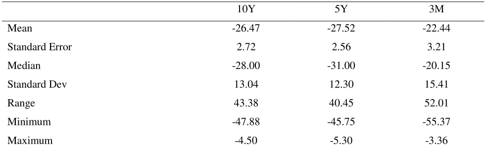
Table 0d: Summary Statistics - After-crisis period
10Y 5Y 3M
Mean -26.47 -27.52 -22.44
Standard Error 2.72 2.56 3.21
Median -28.00 -31.00 -20.15
Standard Dev 13.04 12.30 15.41
Range 43.38 40.45 52.01
Minimum -47.88 -45.75 -55.37
Maximum -4.50 -5.30 -3.36
Notes: The above summary statistics is for the post global crisis and eurozone crisis periods (which overs Q1 2013– Q3 2018). From the table we notice t
Correlation – After-crisis period
10Y 5Y 3M
10Y 1
5Y 0.98 1
In all, some interesting stylized facts arise from the summary statistics. First, the correlation between the short and
long end of the euro basis is relatively lower than the correlation between the long end. Second, the short end of
the basis is more volatile than the long end and has a mostly wider mean value relative to the long end. Third, the
behavior of the euro basis across maturities in the post crisis period is generally similar to the behavior in the
eurozone crisis period. If the long end of the euro basis behaves similarly and are more synchronized, do they also
respond to similar macroeconomic factors? We now move to the next section where we investigate the baseline
model that explains how macroeconomic factors drive the observed behavior of the basis at the long end.
III. Baseline Theoretical Model
To illustrate how relative real output, money supply and spot exchange rate may influence the long-term euro libor
cross-currency basis swap spread, we consider a continuously compounded n-year risk-free interest rates quoted in U.S. dollars and the euro – which is the foreign currency. Let 𝑖 and 𝑖∗be the continuously compounded n-year
risk-free interest rates at time t in the U.S dollars and euro, respectively. Let 𝑆 be the EURUSD spot exchange rate at
time t, where 𝑆 is expressed as the number of units of the euro per unit of the U. S dollars, so an increase in 𝑆 is
understood as an appreciation of the U.S. dollar or a depreciation of the euro, i.e. the U. S. dollar is the numeraire
currency. Furthermore, let 𝐹 denote the n-year forward exchange rate in euro per U. S. dollar at time t. Before we
proceed, let us consider two useful results which will be used to support our exposition.
1. Lemma
By definition,
log(1 + 𝛿) = ∫
1𝜃 1+𝛿
1
𝑑𝜃,
and
𝛿 ≈ 0
such that
𝛿
is in the interval
0 < 𝛿 < 1
, then
1𝜃
≈ 1
for
1 < 𝜃 < 1 + 𝛿
. Hence,
log(1 + 𝛿) ≈ ∫
11+𝛿𝑑𝜃 = 𝛿
. Moreover,
(1 + 𝛿)
𝑛≈ 𝑒
𝑛𝛿for each real
𝑛
. Hence,
for ease of computation, the amount realized from continuously compounding a risk-free interest rate
𝑖
,
0 < 𝑖 < 1,
after
n
periods is approximated as
(1 + 𝑖)
𝑛≈ 𝑒
𝑛𝑖. The same identity holds abroad, i.e.
(1 + 𝑖
∗)
𝑛≈ 𝑒
𝑛𝑖∗.
2. Lemma
If both the U.S. and Euro securities are risk-free and the forward contract bears negligible counter party risk, then
both strategies are the same and thus should yield equivalent payoffs, i.e.
𝑒𝑛𝑖 =𝑒𝑛𝑖
∗ 𝑆 𝐹
1
𝑛 (𝑓− 𝑠) = 𝑖∗− 𝑖 where 𝑓 and 𝑠 are log values.
Thus, if CIP holds, the equality in the above lemma must hold and the cross-currency basis swap spread is trivially zero.
On the other hand, suppose, however, that the CIP fails to hold. Then there is a deviation from covered interest rate
parity and 1𝑛(𝑓− 𝑠) ≠ 𝑖∗− 𝑖. This means that ∃ an 𝑥 ≠ 0, representing the deviations from CIP, such that
1
𝑛(𝑓− 𝑠) = (𝑖∗− 𝑖) + 𝑥 (1.0) 𝑥 is known as the cross-currency basis.
Now, continuing with our previous exposition, suppose there are no barriers to cross border capital and assets flows
between the euro area and the U.S., and a representative agent, with investible U.S. dollars, seeks to exploit the
markets to optimize her financial outcomes. For ease of exposition, let the investible dollars available to the agent
be $1. Two outcomes are possible. First, at time t, she could invest the $1 domestically and generate a total amount
of 𝑒𝑛𝑖 U. S. dollars n years from now. Second, she could exchange her $1 for the euro at the spot exchange rate 𝑆,
enter a swap contract agreement and then invest the 𝑆euro in the eurozone market. At the end of the n years, she
would own a total of 𝑒𝑛𝑖∗𝑆 euros. When she swaps the amount realized in the euro back to the U. S. dollars at the
forward rate 𝐹 previously agreed at time t, this amounts to 𝑒𝑛𝑖∗𝑆 /𝐹 in U. S. dollar terms. This is called synthetic
US dollars.
Meanwhile, suppose that the demand for real money balances in the U.S. and eurozone is characterized as a standard
function of real output and nominal interest rate, where for simplicity, we assume that the nominal interest rate is the
same as the US and euro risk-free interest rates 𝑖 and 𝑖∗ quoted at date t in US dollars and euro. The standard monetary
model can be written as –
𝑚 − 𝑝 = 𝜓1𝑖 + 𝜓2𝑦 (1.1)
𝑚∗− 𝑝∗= 𝜓
1𝑖∗+ 𝜓2𝑦∗ (1.2)
where 𝑚, 𝑝, 𝑖, and 𝑦 denote domestic money supply, price level, interest rate and output respectively in the U.S.,
while asterisks denote variables for the euro area. 𝜓1 and 𝜓2 denote interest rate semi-elasticity of money demand and
income elasticity of money demand, respectively, where 𝜓1> 0 and 𝜓2> 0 in line with Frankel (1979). Except for
interest rates, all other variables are expressed in logarithm.
(𝑚∗− 𝑚) − (𝑝∗− 𝑝) = 𝜓
1(𝑖∗− 𝑖) + 𝜓2(𝑦∗− 𝑦) (1.3)
Meanwhile, standard purchasing power parity implies that, if 𝑠 is the spot exchange rate, then
𝑠 = 𝑝∗− 𝑝, (1.4)
Combining (1.0), (1.3), and (1.4), we obtain
𝑥 = (𝜓1
1−
1
𝑛 ) 𝑠 −
1 𝜓1(𝑚
∗− 𝑚) +𝜓2
𝜓1(𝑦
∗− 𝑦 ) + 𝑓𝑓
𝑡 (1.5𝑎)
which links our variables of interest to the euro cross-currency basis swap spread, 𝑥. The model provides a simple
theoretical framework that leads to testable implications for the long-run relation between the euro cross-currency basis
swap spreads and macroeconomic indicators – relative money supply, relative real output and spot exchange rate.
First derivative of the model with respect to our variables of interest yields 𝜕𝑥
𝜕𝑠 = (
1 𝜓1−
1 𝑛 ) ,
𝜕𝑥
𝜕(𝑚∗− 𝑚) = −
1 𝜓1,
𝜕𝑥 𝜕(𝑦∗− 𝑦) =
𝜓2
𝜓1 (1.5𝑏)
Equation (1.5a) is the model governing the dynamics of the long run links between the euro cross currency basis and
the macroeconomic variables. The dependence of the euro basis swap spreads on the dollar spot exchange rate is in
line with the mirror effect of the dollar on the basis, first emphasized empirically by Avdjiev et al. (2017). However,
apart from Ibhagui (2018), we are not aware of any other studies that link the other variables, i.e. real output and money
supply dynamics, to the basis. Thus, our model simultaneously captures important potential drivers of the euro basis,
some of which have not been investigated for the eurozone in the extant literature.
Assume that2 𝜓
1> 0, and 𝜓2> 1 > 0, we have
𝜕𝑥
𝜕𝑠 = (
1
𝜓1−
1
𝑛 ) <> 0,
𝜕𝑥
𝜕(𝑚∗− 𝑚) = −
1 𝜓1< 0,
𝜕𝑥 𝜕(𝑦∗− 𝑦) =
𝜓2
𝜓1> 0, (1.6)
implying that, ceteris paribus, an increase in relative money supply would worsen CIP deviations in the eurozone and
widen the euro cross-currency basis swap, an increase in relative real output would tighten the deviations while euro
depreciation would either widen or tighten the cross-currency basis swaps. Also, as 𝜓2> 1, we have |𝜓2
𝜓1| > |
1 𝜓1| >
|𝜓1 1−
1
𝑛| > 0, suggesting that the magnitude of the impact of real output on the euro basis should be greater than the
impact of either money supply or exchange rate or the sum of both.
The empirical specification associated with our simple model can be written as
𝑥 = 𝛽0+ 𝛽1𝑠+ 𝛽2(𝑚∗− 𝑚) + 𝛽3(𝑦∗− 𝑦 ) + 𝜀𝑓𝑡 (1.7)
where 𝛽1<> 0, 𝛽2< 0 and 𝛽3 > 0.Equation (1.7) forms the basis for our empirical analysis to test the hypothesis
implied by the model.
IV. Data and Empirical Methodology
a. Data
The data for this study consists of quarterly observations for the cross-currency basis, the nominal exchange rate
(euro per U.S. dollar), the euro area money supply relative to the U.S., and euro real output relative to the U.S. from
Q1 2003 to Q3 2018, selected based on data availability for all variables. The cross-currency basis and nominal
exchange rate series are from Bloomberg data manager, and the money supply and real GDP series are from the
Federal Reserve Economic Data (FRED) economic data. Except for the cross-currency basis, all variables are
measured in log-levels.
b. Empirical Methodology
We focus on the long-run relation between our variables of interest – which are the macroeconomic factors – and the
long end of the euro cross-currency basis. In our time series analysis, we first provide exhaustive evidence that a
cointegrated relation exists among the components of the vector [𝑥, 𝑠, (𝑚∗− 𝑚), (𝑦∗− 𝑦 )] which enables us to
estimate and uncover the long-run relation among the variables, particularly how the macroeconomic factors impact
the euro cross-currency basis swap spreads in the long run. We estimate the cointegrating equation using the
appropriate time series estimators for cointegrated system of variables. These are the dynamic ordinary least squares
(DOLS), fully modified ordinary least squares (FMOLS) and canonical cointegrating regression (CCR). We also
include the ordinary OLS for comparison.
We begin the empirical analysis by first investigating the integration properties of our series.
c. Unit roots
We first investigate the integration properties of [𝑥, 𝑠, (𝑚∗− 𝑚), (𝑦∗− 𝑦 )] using the well-known augmented
dickey fuller (ADF) unit root test, as well as the DF-GLS and 𝑀𝑍𝛼 unit root tests which have been shown to have
good size and power properties Ng and Perron (2000). Table 1 reports the results for the unit root tests. Column (1)
of the first row of Table 1 shows the variable tested in levels; column 2 of the first row shows whether a linear trend
was included in the unit root tests while the second row reports the first difference. All our specifications include a
constant term.
We designate the variables in Table 1 as I(1) or I(0) using the following decision rule: If at least two of the tests
5 percent significance level, then we designate the corresponding variable I(0). If at least two of the tests do not
[image:15.612.46.612.96.252.2]reject the null hypothesis of nonstationarity at the 10 percent level or better, we designate the variable as I(1).
Table 1: Unit root test results
Variable in level ADF DF-GLS 𝑴𝒁𝜶 Variable in level (with trend)
ADF DF-GLS 𝑴𝒁𝜶 Decision
𝒙 -0.59 -1.34 -3.63 𝒙 -1.71 -2.54 -12.91 I(1)
𝒔 -2.27 -1.59 -4.42 𝒔 -2.66 -1.94 -6.08 I(1)
𝒎∗− 𝒎 -0.15 -0.33 -0.39 𝒎∗− 𝒎 -1.92 -0.85 -0.88 I(1)
𝒚∗− 𝒚 -0.91 0.96 0.63 𝒚∗− 𝒚 -1.64 -1.61 1.29 I(1)
Variable in first difference ADF DF-GLS 𝑴𝒁𝜶 Variable in first difference (with trend)
ADF DF-GLS 𝑴𝒁𝜶
𝒙 -3.34*** -10.09*** -28.45*** 𝒙 -3.31*** -10.09*** -28.45*** I(0)
𝒔 -7.67*** -6.11*** -28.77*** 𝒔 -7.71*** -7.43*** -30.36*** I(0)
𝒎∗− 𝒎 -2.84*** -2.86*** -8.90*** 𝒎∗− 𝒎
-3.23*** -3.17*** -10.01*** I(0)
𝒚∗− 𝒚 -7.43*** -3.57*** -16.59*** 𝒚∗− 𝒚
-7.35*** -7.00*** -30.08*** I(0) *, **, *** indicate significance at the 10, 5, and 1 percent levels, respectively; (trend) indicates test allows for both a constant and stationarity around a linear trend.
1. ADF critical values at the 10, 5, and 1 percent critical values are -2.59, -2.91 and -3.56, respectively; when a linear trend is included, the 10, 5, and 1 percent critical values become -3.17, -3.48 and -4.12, respectively.
2. DF-GLS critical values at 10, 5, and 1 percent levels are -1.61, -1.95 and -2.60; with linear trend included, they become -2.86, -3.15 and -3.73 respectively.
3. 𝑀𝑍𝛼 critical values at 10, 5, and 1 percent levels are -5.70, -8.10 and -13.81; with linear trend included, they become -14.20, -17.30 and -23.80 respectively 4. 𝐻0 in each case is the null hypothesis of nonstationarity or unit root.
Based on the unit root test results in Table 1, we conclude that all four of the variables, [𝑥, 𝑠, (𝑚∗− 𝑚), (𝑦∗− 𝑦 )]
are I(1). In this scenario, our long-run model strictly requires cointegration between the integrated variables over our
sample. Since these variables are all I(1), in the next subsection, we test for a cointegrating relationship among these
four variables. We report cointegrating estimates for the variables in Table 2.
d. Cointegration test results and coefficient estimation
Table 2 reports the Johansen trace and maximum eigen value cointegration tests. The test clearly indicates that the
null hypothesis of no cointegration is rejected, suggesting cointegrating relationship for the cross-currency basis and
Table 2: Johansen Cointegration tests
No trend
𝐻0 Trace Statistic 5% Critical Value Maximum Eigen Statistic 5% Critical Value
𝑟 = 0 57.22*** 47.21 37.86*** 27.58
𝑟 ≤ 1 28.25 29.68 19.25 21.13
𝑟 ≤ 2 11.64 15.41 1.69 14.26
𝑟 ≤ 3 1.00 3.76 2.82 3.84
With trend
𝐻0 Trace Statistic 5% Critical Value Maximum Eigen Statistic 5% Critical Value
𝑟 = 0 51.14*** 54.64 38.82*** 32.12
𝑟 ≤ 1 27.86 34.55 24.92 25.82
𝑟 ≤ 2 15.35 18.17 10.18 19.38
𝑟 ≤ 3 5.05 3.74 4.32 12.52
[image:16.612.73.575.301.428.2]r denotes the number of cointegrating vectors. The optimal lag lengths for the VARs were selected by minimizing the AIC. At this lag, the VAR produces results that exhibit no serial correlation. *** indicates rejection of the null hypothesis of no-cointegration at 5% level of significance or better.
Table 3 - Estimation of Coefficient of Cointegrating Equation
DOLS FMOLS CCR Static OLS
𝒔 -2.98*** -1.87*** -1.77*** -1.07**
(2.62) (2.46) (2.47) (2.25)
𝒎∗− 𝒎 -5.11*** -3.39** -3.34*** -2.32***
(2.56) (2.49) (2.68) (3.18)
𝒚∗− 𝒚 9.44*** 7.70*** 7.79*** 8.32***
(3.21) (3.64) (4.05) (12.16)
𝑹𝟐 0.75 0.43 0.33 0.52
Figures in brackets are t-statistics. (***) and (**) indicate statistical significance at the 1% and 5% level, respectively. Results are reported in
per basis point change in each of the original independent variable so that a 100 basis points change (a percentage change) in the original
independent variable will correspond to the reported estimated coefficients multiplied by 100. We specific DOLS (-1, 1).
Table 3 presents the empirical results for the estimation of the coefficients of the regressions, based on the
specification in equation (1.7). Overall, a number of stylized features of the data, consistent with our original model,
emerge from these regressions. First, there is a positive and strongly significant long-run relation between the
cross-currency basis swap spread and relative real output in the euro area, providing support for the existence of a
tightening effect of real output increases on the long-end of the euro basis. The magnitudes of the coefficients across
the different estimators are remarkably similar and in line with those predicted by the benchmark model. The size of
the relative real output effect on the basis is economically and statistically significant: according to the estimated
point coefficients, a 10-basis point increase in euro real output relative to the US implies a long-run basis tightening
of about 77 to 94 basis points. Second, the relation between cross-currency basis and relative real output is stronger
supply, again confirming the deduction from our simple model. This can be seen to be true across all estimators
employed, even across the OLS estimator which is especially the least efficient of all the estimators.
The results also show that there is a significant negative effect of euro depreciation on the cross-currency basis and
this result stands for the entire estimators, suggesting that a 10-basis point depreciation of the euro would widen the
cross-currency basis by about 11 to 30 basis point in the long run. In fact, the negative relation turns out both
statistically and economically very significant. Finally, relative money supply increases are associated with basis
spread widening as seen in Table 3, and the relation is economically and statistically significant. A 10-basis point
rise in euro money supply relative to the US would widen the euro cross currency basis by about 23 to 51 basis points
in the long run.
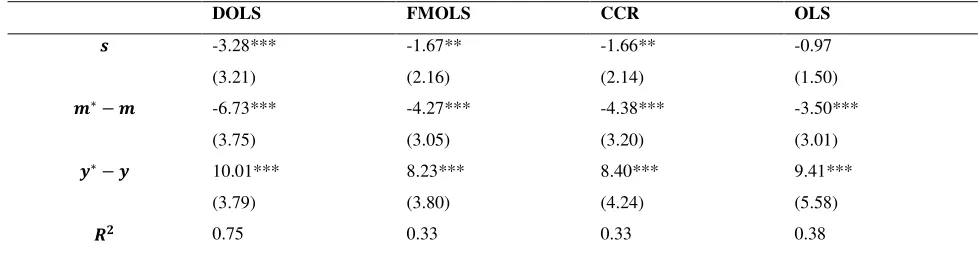
As a robustness check, we replace the 10-year basis with 5-year basis and re-estimate the model to check whether
our main results are robust to the choice of the long end of the euro basis. The result, reported in Table 4, shows that
previous findings are unaltered as all effects preserve their previous inclination and remain very significant
statistically and economically. Also, the magnitude of the effect of relative real output continues to be greater than
the magnitude of relative money supply, exchange rate as well as their sum, suggesting that an increase in relative
real output in the euro area is responsible for most of the tightening in the long end of the euro basis in the long run
[image:17.612.80.569.355.493.2]and more than offsets the combined widening pressures from money supply increases and currency depreciations.
Table 4: Robustness with an alternative long end basis – 5-year
DOLS FMOLS CCR OLS
𝒔 -3.28*** -1.67** -1.66** -0.97
(3.21) (2.16) (2.14) (1.50)
𝒎∗− 𝒎 -6.73*** -4.27*** -4.38*** -3.50***
(3.75) (3.05) (3.20) (3.01)
𝒚∗− 𝒚 10.01*** 8.23*** 8.40*** 9.41***
(3.79) (3.80) (4.24) (5.58)
𝑹𝟐 0.75 0.33 0.33 0.38
Figures in brackets are t-statistics. (***) and (**) indicate statistical significance at the 1% and 5% level, respectively. Results are reported in
per basis point change in each of the original independent variable so that a 100 basis points change (a percentage change) in the original
independent variable will correspond to the reported estimated coefficients multiplied by 100.
Fig. 2 presents graphs of the euro basis deviations from the level implied by our simple model for the four estimators
reported in Table 3. Vertical lines are drawn for the periods Q4 2007 and Q4 2012 to roughly depict different
historical regimes in the global financial markets: i) commencement of the global financial crisis and thereafter the
euro crisis, and ii) the end of the euro crisis and global financial crisis. The deviations based on each estimator have
a strong tendency for mean-reversion as shown in Fig 2. It is also from Fig 2 that the deviations from the level
implied by the identified macroeconomic fundamentals can be sizeable. However, except in few instances, they are
generally not very persistent. Consequently, it is plausible to detect the long-run relationship between the
Note that the period prior to the global financial crisis, particularly the 2004 to the 2006 period, stands out in Fig 2
as a period where the euro cross-currency basis diverges considerably from the underlying macroeconomic
fundamentals in our model. The euro cross-currency basis was little and mostly positive during this period, as is
widely known in the literature. Also, the deviations tend to be quite substantial and persistent, on average, in this
period and towards the end of the eurozone crisis. Because of this, it will be tough attempting to detect the long-run
[image:18.612.71.575.150.531.2]relationship between the cross-currency basis and macroeconomic fundamentals using data from these periods alone.
Fig 2: Deviations of the basis from the long run level implied by our simple model
Note: Vertical lines are drawn for the periods Q4 2007 and Q4 2012 to roughly depict different historical regimes in the global financial markets: i) commencement of the global financial crisis and thereafter the euro crisis, and ii) the end of the euro crisis and global financial crisis
To summarize the results of this section, we find considerable support for the predictions of our simple stylized
model of the long-run impact of macroeconomic fundamentals on the euro cross-currency basis swap spreads. Also,
Fig. 1 suggests that long data spans, which include substantial periods of negligible and less persistent deviations
from the identified macroeconomic factors, will generally be important to successfully detect the long-run
equilibrium relationship between macroeconomic variable and the basis implied by our stylized model. -40 -30 -20 -10 0 10 20 30 3/1 /200 3 2/1 /200 4 1/1 /200 5 12/ 1/20 05 11/ 1/20 06 10/ 1/20 07 9/1 /200 8 8/1 /200 9 7/1 /201 0 6/1 /201 1 5/1 /201 2 4/1 /201 3 3/1 /201 4 2/1 /201 5 1/1 /201 6 12/ 1/20 16 11/ 1/20 17
DOLS
-40 -30 -20 -10 0 10 20 303/1/2003 4/1/2004 5/1/2005 6/1/2006 7/1/2007 8/1/2008 9/1/2009
10/1/2010 11/1/2011 12/1/2012 1/1/2014 2/1/2015 3/1/2016 4/1/2017 5/1/2018
FMOLS
-40 -30 -20 -10 0 10 20 303/1/2003 4/1/2004 5/1/2005 6/1/2006 7/1/2007 8/1/2008 9/1/2009
10/1/2010 11/1/2011 12/1/2012 1/1/2014 2/1/2015 3/1/2016 4/1/2017 5/1/2018
CCR
-40 -30 -20 -10 0 10 20 30 3/1/2003 4/1 /20 045/1/2005 6/1/2006 7/1/2007 8/1/2008 9/1/2009 10/1/2010 11/1/2
01
1
12/1/2012 1/1/2014 2/1/2015 3/1/2016 4/1/2017 5/1/2018
We now provide some views on the process through which the identified macroeconomic factors influence the euro
basis in the long run. The tighter basis from increased eurozone real output suggests that in the long run, when
eurozone real output improves relative to the US, the eurozone becomes an attractive investment destination which
in turn induces demand for euro securities, particularly from US dollar entities. The demand for euro assets from US
dollar-based entities – with proceeds hedged into US dollar libor – encourages the issuance of euro denominated
bonds which accelerates the issuance of euro liabilities – i.e. reverse yankee bonds – by foreign issuers who
subsequently swap the euro liabilities into US dollars.
As demand for euro assets increases, euro spreads tend to shrink, and the basis tightens. From the supply side, this
encourages the issuance of euro liabilities as a combination of lower spreads and tighter basis is favourable to euro
issuers looking to swap to US dollars as this reduces their funding costs. Although the demand for euro assets stokes
issuance of euro denominated bond, our results suggest that in an improving eurozone economy, the issuance of euro
denominated bonds tends to fall behind the overall demand for euro assets hedged to dollars. The relatively lower
barrier could be driven by barriers to issuance which foreign entities often face. It could also be driven by strategic
decisions to limit issuance amid rising demand for euro securities – it is well known, issuers do not respond
proportionately to all demand for euro assets. Thus, supply of hedging activities – associated with demand for
dollar-hedged euro assets – outstrips demand for hedging activities, associated with issuance of euro liabilities swapped
into dollars, consequently tightening the cross-currency basis.
In all, our results reveals that even though tighter cross-currency basis should increase funding activities in the euro
area for foreign entities seeking dollars as it becomes cheaper to obtain dollars via euro, if the eurozone real output
remains relatively more favourable, then demand for euro assets hedged to dollars would rise at a faster pace than
issuance or funding in euro, causing the basis to tighten. This mechanism plausibly explains how an increase in
eurozone real output relative to the US can tighten the euro cross-currency basis.
Turning to relative money supply, a rise in eurozone money supply relative to the US, which signals a more
accommodative or less restrictive monetary stance in the eurozone, narrows eurozone spreads. This increases/induces
an increase in funding activities as foreign issuers increase the issuance of euro liabilities to latch on the lower cost
of euro debt. The relative abundance of money in supply attracts the interest of issuers who seek easy access to
abundant euro. Euro-based issuers might issue locally to take advantage of the abundant and cheaper euro for onward
carry trades and other high-return investments, with proceeds hedged into euro. Foreign issuers whose end currency
is the US dollar, would issue with the sole aim of swapping to the final currency of choice,mostly the US dollar.
Both activities would elevate demand for hedging activities
As the euro liabilities are swapped to the dollar, this increases the demand for hedging activities and puts a downward
pressure on the euro cross-currency basis swap spread. The increased issuance of euro liabilities is not driven by
demand for euro securities. Instead, it is driven by the availability and perceived reduction in the cost of euro debt
Since the supply of hedging activities, i.e. demand for euro assets hedged to dollars, becomes limited, this creates an
imbalance wherein demand for hedging dominates supply of hedging. The demand for euro assets hedged to dollars,
and hence supply of hedging activities, shrinks because the loose monetary stance generally makes it unattractive
for US dollar-based investors to demand or hold euro assets hedged into dollar libor. This lowers their demand for
euro securities as they seek better returns elsewhere. In this instance, the imbalance tilts towards a much higher
demand for hedging activities from the euro liability issuers relative to the supply of hedging activities from US
dollar-based holders of euro assets. Consequently, the euro cross-currency basis widens.
If the euro basis widens considerably, this may increase the funding cost associated with swapping euro into dollars
which, all else unchanged, should limit the issuing and swapping of the euro and possibly stabilize or even tighten
the basis. However, if the relative money supply continues to rise, credit spreads would tighten further, issuers would
remain attracted to funding via the euro, and the euro basis would continue to widen.
Moving now to the exchange rate, the result is in line with the view that an appreciation of the dollar is associated
with a wider cross-currency basis. Viewed from the perspective of supply of hedging activities (that is, the demand
for foreign assets), Avdjiev et al. (2017) argues that the US dollar serves as a risk barometer, “…. the dollar is a key
barometer of risk-taking capacity in global capital markets”. A stronger dollar reduces cross-border lending in dollars
as the risk of lending in dollars increases when the dollar strengthens relative to foreign currencies. This is because
a stronger dollar means foreign, non-dollar, entities become more burdened and could fail to meet maturing dollar
obligations; the dollar obligations become elevated in foreign currency terms even when the value of the obligations
in dollars remains unchanged. This reduces cross-border dollar lending and hence reduces demand for euro securities,
lowering supply of hedging activities.
From the issuance side, because of the appreciation of the dollar, more euro liabilities would need to be issued and
dollar-swapped to get the same amount of dollars. This increases the issuance of euro denominated bonds and puts
upward pressure on demand for hedging activities. In this scenario, demand for hedging dominates supply of hedging
as there are more euro liabilities being created (to be swapped for the same amount of dollars) than assets being
demanded (given lower dollar inflows and lower cross-border lending in dollars), resulting in lower demand for euro
assets from US dollar investors and consequently widens the euro basis.
V. Convergence to Long Run- Error-correction Mechanism
In this section, we seek to gain insight into how the long-run equilibrium is restored between the basis and the
identified macroeconomic variables by estimating vector error-correction models. By the Granger representation
long-run value. Accordingly, by inspecting the error correction mechanism (ECM), insight is gained into which variables
[image:21.612.73.579.99.304.2]endogenously adjust to ensure convergence to the long-run relation.
Table 5: Error correction coefficients (ECM) estimate
(1) (2) (3) (4)
A. 10-year basis
𝑥 𝑠 𝑚∗− 𝑚 𝑦∗− 𝑦
𝑬𝑪𝑴 -0.1382* -0.0002 0.0001 0.0001***
(1.78) (1.13) (1.10) (4.29)
𝑹𝟐 0.05 0.04 0.11 0.32
B. 5-year basis
𝑥 𝑠 𝑚∗− 𝑚 𝑦∗− 𝑦
𝑬𝑪𝑴 -0.1377* -0.0002 0.0001* 0.0001***
(1.71) (1.11) (1.73) (4.54)
𝑹𝟐 0.05 0.04 0.14 0.34
Note: ,*,**,*** indicate significance at the 10, 5, and 1 percent levels, respectively. A. is based on the 10-year basis and B. the 5 year basis
Table 5 reports the dynamic impact of the error correction term on the changes of each of the variables in the
cointegrated vector. We can see that for both the 5-year and 10-year basis, which are our measures for the long-end
of the euro basis, it is the euro basis that is the only predominant adjusting variable. In both cases, the error-correction
coefficient is negative and significant while for the other variables, the coefficients are mostly insignificant. This
implies that the macroeconomic variables are weakly exogeneous for the euro and when deviations from the implied
long-run equilibrium occur in the Eurozone, it is predominantly the basis, and not the macroeconomic factors, that
adjusts to restore long-run equilibrium over our sample period. In both cases, the speed of adjustment implies a
half-life for basis swap equilibrium misalignments of about 5 quarters, meaning that it should take around 5 quarters for
one half of shifts away from the equilibrium implied by our model to be restored. With respect to the other variables,
the ECM variable has no explanatory power for the dynamics of the relative money supply and exchange rate
positions, and actually has a positive sign in relative money supply and real output equation. Overall, the similar
adjustment mechanisms at work for both tenors over the last decade reflect robustness of our findings for the
VI. Dynamic Interdependencies using Vector Autoregressions
After establishing the long-run relationship between the euro basis and exchange rate, relative real output and
relative money supply, we now turn to the last part of our analysis where we investigate the dynamic
interdependencies between the euro basis and each of the identified drivers. Thus, in this section, we want to study
the effects of exchange rate shocks, money supply shocks and real output shocks on the cross-currency basis swap
spread. We do not impose any specific restrictions in our VAR. Instead, we allow the variables to speak for themselves.
We consider different orderings of our variables in a generalized impulse response (GIRF) framework which yields
results invariant to the chosen ordering. One major merit of the GIRF is that it generates unique impulse responses and
singles out shocks without resorting to restrictive identifying restrictions.
In order to explore the dynamic interdependencies between the basis and the main variables of interest, we
estimate a 4-variable VAR for 𝑍𝑡 = [∆𝑥𝑡, ∆𝑠𝑡, ∆(𝑦𝑡∗− 𝑦𝑡), ∆(𝑚𝑡∗− 𝑚𝑡) ]′ , specified as
𝐴0𝑍𝑡= 𝐵(𝐿)𝑍𝑡−1+ 𝐶𝑋𝑡+ 𝑢𝑡 (1.8)
where 𝑍𝑡 is a 4-variable vector of our endogenous variables, where the endogenous variables are as previously
defined, 𝐴0 is the matrix of contemporaneous coefficients, 𝐵(𝐿) is a polynomial of lagged coefficients, 𝑋𝑡 is a
vector with intercepts and linear trends, and 𝑢𝑡 is a vector of structural innovations.
Pre-multiplying by 𝐴0−1 gives the model in reduced form as
𝑍𝑡 = 𝐽(𝐿)𝑍𝑡−1+ 𝐾𝑋𝑡+ 𝑣𝑡 (1.9)
where 𝐽(𝐿) = 𝐴0−1𝐵(𝐿), 𝐾 = 𝐴0−1𝐶, 𝑣𝑡 = 𝐴0−1𝑢𝑡
Figure 5 reports the cumulative response for a one-time shock to changes in exchange rate, relative real output and
relative money supply. In general, the impulse responses are quantitatively different. Figure 5 displays the
cumulative impulse responses from our 4-variable specification and shows the effect of a positive shock to
exchange rate, interpreted as a stronger dollar or weaker euro, widens the basis. The cumulative impulse response
function plots the accumulation of the impact of the shock to our variables across time, unlike the impulse response
function which provides the impact of a shock at a single point in time. We concentrate on the dynamics of the shocks
Figure 5: Cumulative impulse response functions of EUR/USD cross-currency basis swap spread (𝒙) to a shock in US dollar exchange rate (𝒔), relative money supply (𝒎∗− 𝒎) and relative real output (𝒚∗− 𝒚 )
Response of 𝒙 to 𝒙 Response of 𝒙 to 𝒔
Response of 𝒙 to 𝒎∗− 𝒎 Response of 𝒙 to 𝒚∗− 𝒚
The top left graph shows that the basis is positively affected by a one standard deviation shock of itself upon impact. It
tightens on impact. As time progresses, the basis continues to be positively affected by this one-time shock on itself.
The top right graph shows that the basis is negatively affected by a one standard deviation exchange rate shock upon
impact, and as time goes on the basis continues to be negatively affected by the shock. The responses show that the
exchange rate has a persistently negative and significant impact on the basis on impact and these negative
dynamics accumulate over time. This result is robust to alternative ordering of the variables estimated by the
generalized impulse response. The estimated negative impact is visible and remains significant for several quarters
after the occurrence of the shock. The bottom left, and right graphs show the effect on the basis of a shock to relative
real output and money supply, respectively. The real output shock positively affects the basis and this benefit is
marginal, quickly levels off about 6 quarters after the shock and largely unchanged over time. The money supply shock
continually remains in the negative. Both money supply and real output shocks have a statistically negligible effect on
the basis even on impact.
In all, we have shown that the exchange rate shock decreases the basis permanently while shocks to real output
increases the basis. We also see that the basis first increases in response to a money supply shock but falls below
zero, eventually decreasing the basis over time. In general, a shock to the exchange rate tends to produce a higher,
significant and more persistent negative effect on the basis than a shock to either of the other variables. These
results are largely robust to alternative ordering of the variables and the inclusion a deterministic time trend. In
general, the generalized impulse responses, which we employed, are invariant to the order of the variables in the
VAR system. Our main conclusion in this exercise on the dynamic interdependencies is that that irrespective of the
component, the response of the basis due to exchange rate shocks is more significant and persistent than those
caused by real output or money supply shocks and factors driving fluctuations are potentially largely external.
Juxtaposing with the long run evidence, our result proposes that while exchange rate has the least effect on the
long-end of the euro basis in the long run, the basis effects of exchange rate shocks in the short run appear to be
more persistent and relatively more pronounced.
VI. Relation to other studies
Although to our knowledge, there are no studies that have specifically addressed the links between our identified
macroeconomic variables and the cross-currency basis in a major monetary union such as the eurozone, we would
attempt to make a comparison of our findings with those obtained by the few related studies available.
Using a collection of G10 countries, Avdjiev et al. (2017) estimated a panel regression of the cross-currency basis
on the dollar exchange rate, with the variables expressed as changes in levels over the sample period. They obtained
a strong evidence of a wider basis when the dollar appreciates, with a significantly negative coefficient across most
currencies. In this paper, we have estimated the long-run links not only between exchange rate and cross-currency
basis for a longer span but also, we have done this in the presence of plausible macroeconomic drivers of the basis.
This enables us to control, as suggested by our theoretical model, for the effects of relative money supply and relative
real output. This is important, especially in view of the links between these variables and the exchange rate, the
strong and significant effect of relative money supply and relative real output on the euro basis at the long end, and
the fact that dollar exchange rate is not necessarily the only important driver for the basis in the long run. This is
relevant as it enables us to obtain the effect of each variable on the cross-currency basis whilst controlling for the
presence of the other variables. We found the effect of relative real output on the basis to be much stronger, and the
effect of relative money supply and exchange rate to be much weaker in our framework
With respect to long-run cointegrating relation, Baran and Whitzany (2017) estimates the long-run drivers of the
euro cross-currency basis, including in their cointegrating vector the exchange rate, measures of credit risk, volatility
index and credit spreads. They find that the cross-currency basis tends to be tighter in the long run when the euro
strengthens relative to the dollar. However, their study excludes standard macroeconomic variables as have been
the variables included in their cointegrating vectors as potential drivers of the basis. Du et al. (2017) estimate the
effect of regulation on cross-currency basis and find that the more stringent regulation that followed the crisis
explains why the cross-currency basis has persisted, and CIP deviations have not been arbitraged away. The key
issue in these studies is the complete neglect of the effects of other plausible macroeconomic factors on the
cross-currency basis. Moreover, ignoring these factors have possibly been responsible for the often-low explanatory power
of the drivers of the basis advanced so far in the literature.
Our paper is the first that directly studies the long-run relationship between the euro cross-currency basis and
standard macroeconomic variables in the eurozone. The only other paper that we are aware of, that specifically
studies the long-run drivers of the euro basis, is Baran and Whitzany (2017). However, their framework is purely
empirical, focuses on the short to mid end of the euro basis and does not provide a theoretical motivation. We present
instead a new empirical evidence motivated by a simple theoretical framework which enables us to directly test the
implications of our hypothesis without losing much degree of freedom in an environment of limited data, as that
would be the case if we aimlessly handpicked regressors as potential drivers of the basis. In a recent work, Ibhagui
(2018) derives a model based on the standard monetary model. This paper, which focuses on the eurozone, rather
than on a panel of countries like Ibhagui (2018), draws from that model as a benchmark to investigate the significance
of the identified macroeconomic factors for the euro basis in the long run. Thus, our results are specific to the
eurozone and we make no claim that they extend to other countries or currencies given the heterogeneity among
countries, even those with developed financial markets.
Finally, this paper has investigated long-run relations between the basis and macroeconomic factors, with a focus on
the eurozone. Our promising results suggest directions for future research. Thus, our next line of action would be to
extend this country specific research to include other G10 currencies and the broader emerging markets even as we
also seek to analyze the short run dynamic linkages between the basis and their associated macroeconomic drivers.
In countries for which there is support for our model, it would be interesting to compare the similarity of the support
to the eurozone and to examine the dynamics of the adjustment process to the long-run equilibrium relation implied
by the model by studying metrics such as the panel impulse responses and variance decompositions for the
cross-currency basis and macroeconomic fundamentals in these countries. It would also be interesting to undertake a
research to build a dynamic stochastic general equilibrium (DSGE) model that can replicate the dynamics of these
variables and extend this line of research to emerging market economies. However, the task could be complicated
by patchy data as the derivatives markets of some of these EM economies are much less developed. This paper has
taken the U.S. as the numeriare. Future research could utilize other major countries variables or even the eurozone
as the numeriare and investigate whether our model has support as a long-run anchor for characterizing the
cross-currency basis. Finally, it is plausible that the divergence of the basis from the identified underlying macroeconomic
factors could exhibit nonlinearity in reversion to mean. Thus, issues pertaining to exploring this possibility for the
euro zone and other countries for which we find support for our model have major relevance for derivatives policy
makers and rank high in the priority list for future research efforts in untangling the long-run macroeconomic anchors