Liquidity of General Motor Company due to their Internal and External factor

Munich Personal RePEc Archive

Liquidity of General Motor Company

due to their Internal and External factor

Lim, Wen Yi

Universiti Utara Malaysia

24 November 2019

Liquidity of General Motor Company due to their Internal and External factor

Lim Wen Yi

Universiti Utara Malaysia

ABSTRACT

GM is also known as General Motors Company is America famous high-end automobile producer. In September 2019 GM facing a strike by its employees about terms in a contract. To get employees back to work after more than a month on strike GM offers a 3 percent pay rise for two years of the four-year contract, and similar-sized bonuses for two years. They also hammered out a deal to make permanent temporary workers with three years on the job. This strike cause GM factories paralyzed across the country with losing $90 million a day and thousands of auto workers are draining their savings since they stop working on 16 September. This study aims to find out the internal and external factors affect liquidity in General Motor Company from 2014 to 2018. 5 years annual report of General Motors Company which starts from 2014 to 2018 is to calculate the relationship by using this formula (return on asset, current ratio, quick ratio, average-collection period, debt to income, operational ratio and operating margin) In this study, I have found out that strong corporate governance is applied in GM. However, it founds that quick ratio have a significant relationship with the liquidity of GM.

1.0: INTRODUCTION

1.1 Background of company

General Motors Company can defined as GM. 1908 GM formally established and turn into world’s largest automobile company. General Motors has been pushing the limits of transportation and technology for over 100 years. The multinational company from the United States has offered secured jobs to millions of people around the world. It was originally founded by William C. Durant on September 16, 1908 as a holding company. The GM has its base in nearly 35 advanced countries and manufactures trucks and cars. The cars and trucks are sold under different brand names such as Buick, Cadillac, Chevrolet, GM Daewoo, Hummer, Opal, Pontiac, etc.

In 1907 has a financial crisis and stock market panic but for William Durant, it is a golden opportunity to let him managed to take over many car companies that built car parts as well as car accessories. This process gave birth to General Motors in 1908. The history of General Motors thus began its journey in the automobile market. The successful period in history General Motor is from 1915 to 1920, in this period that Cadillac became successful around the world and the Chevrolet Motors created history in the automobile world. There were many ups and downs but still, GM stood firm in all situations. The GM had a lot of competition from Ford and Chrysler.

The Ford cars became the first choice of the people it makes GM had to face great challenges and make certain changes to compete with Ford. The genius engineer Alfred Sloan accepted this challenge and was quite successful in his attempt. The attractive colors, excellent features, and comfort brought GM back into the market. Many schemes were launched in the interest of the public, but the days never remain the same in 1929 the financial crisis was again set back in the history of General Motors but fortunately, GM managed to bounce back in 1930.

They included Electro-Motive Corporation, the internal combustion engine car builder. This step gave birth to diesel and petrol-fueled cars that were more efficient and comfortable. The year 1955 is another landmark in the history of General Motors. This year, GM became the first company to generate more than a billion dollars in a year. Anyway, the history of General Motors suggests that the company has gone through many difficult stages in the past. They have never given up and have always found their way back in the international market.

1.2 Aim

Propose of this study is to find out the liquidity of General Motor Company due to its internal and external factors.

1.3 Research Objectives:

2. To determine the relationship between external factor and liquidity of GM.

3. To determine the relationship between internal and external factor with liquidity of GM.

1.4 Research Question:

1. What is the relationship between internal factor and liquidity of GM? 2. What is the relationship between external factor and liquidity of GM?

2.0 LITERATURE REVIEW

As reported by, Corporate Governance and development interpretation that definitions of corporate governance very widely. They divided into two categories. The first definitions is related to a set of behavioral patterns—the actual behavior of corporations, in terms of such measures as efficiency, growth, treatment, financial structure, and performance of shareholders and other stakeholders. While the other is concerned with the normative framework—the rules under which firms are operating, with the rules coming from such sources as the legal system, the judicial system, financial markets, and factor (labor) markets.

John E. CoreRobert W. Holthausen, 1999 has been mentioned that the academic literature on corporate governance is to inspect the efficacy of alternative ownership structures and alternative structures for the board of directors. While the failure of certain governance structures is mounting evidence to motivate managers to improve firm performance, the empirical evidence to date is mixed and gives little coherent evidence for the shape of an optimal governance structure.

Refer to Williamson 1984, corporate governance structures are the set of institutional arrangements that objective is to align the interests of management and residual risk bearing shareholders to serve to economize on the transaction costs that accompany the specialization of organizational functions.

The BCBS definition of operational risk (BCBS, 2006) and the evidence provided by the literature (e.g. Cummins et al., 2006, Chernobai et al., 2011, Wang and Hsu, 2013) show that operational risk event announcements3 reveals serious problems in internal control systems, behavior of management and employees, and ultimately weak corporate governance mechanisms in financial firms. These problems uncovered in the announcements have important ramifications for investors as they indicate information that could potentially affect their expected return and variance (Markowitz, 1952), whilst allowing for investors to perceive their potential risk exposure to the event itself by

taking into consideration the levels of ‘controllability’ the institution has at its disposal to

limit exposure (March and Shapira, 1987, Slovic, 1987, Weber and Milliman, 1997).

Based on the standard definition, we divide operational risk into two types. Type one

corresponds to the risk of a loss due to the firm’s operating system, i.e., a failure in a

transaction or investment, either due to an error in the back office (or production) process or due to legal considerations. And, type two corresponds to the risk of a loss due to incentives, including both fraud and mismanagement.2 The second type of operational

risk represents an agency cost, due to the separation of a firm’s ownership and

management. Agency costs are recognized as a significant force in economics, and they have received significant study in the corporate finance literature as key determinants of

types of operational risk losses occur with repeated regularity, and they can be small or catastrophic.

Liquidity risk sent out from the nature of the banking business, from the macro factors that are exogenous to the bank, as well as from the financing and operational policies that are internal to the banking firm. The nature of sharia compatible contracts is an additional source of liquidity risk for Islamic banks, especially if the conventional financial infrastructure is maintained. Banks provide maturity transformation. Taking deposits that are callable on demand or that on average has shorter maturity than the average maturity of the financing contracts they sell. Liquidity insurance to the depositors will provide while maturity transformation, which is valued by them, and the liquidity risk will expose to banks. Since banks specialize in maturity transformation they take pool deposits and take care to match their cash inflows and outflows to solve the liquidity risk they face.

Individuals in advanced capitalist societies — OECD members, plus a few others including Israel and Argentina — are increasingly exposed to market risks. Cuts in unemployment insurance, privatization of state pension schemes, the decline of defined-benefit private pension plans, tightening of bankruptcy laws, and other developments have shifted market risks from collective agents — the state and large corporations — to individuals. In the U.S., this trend of increasing exposure to market risks is highlighted by the dramatic upturn in personal bankruptcy filings and increased income volatility in the middle class.1 Even social democracies such as Sweden have cut back on welfare state benefits by privatizing pensions.

Market risk, in turn, can be classified into interest-rate risks, equity risks, exchange rate risks, commodity price risks, and so on, depending on whether the risk factor is an interest rate, a stock price, or another random variable. Market risks can also be distinguished from other forms of financial risk, particularly credit risk (or the risk of loss arising from the failure of a counterparty to make a promised payment) and operational risk (or the risk of loss arising from the failures of internal system or the people who operate in them).

especially those who qualified in the global market and have to comply with foreign environmental standards and rules.

3.0: METHODOLOGY

3.1 Introduction

According to the book - Research Methodology: Methods and Techniques it means consisting of indicate the problem, formulating a hypothesis, gathering the facts or data, analyzing the facts and reaching certain conclusions either in the form of solutions towards the concerned problem or in certain generalizations for some theoretical formulation.

3.2 Sampling Technique

General Motor Company will publish annual report every year and 2014 until 2018 has been chosen as sample to study the relationship of dependent variable (current ratio) and independent variables (ROA, quick ratio, average collection period, operating margin, operational ratio, unemployment rate, CGI, standard deviation, exchange rate, GDP and interest rate). The multiple regression analysis can be shown as follows in the equation:

Equation 1: ai + a1CR + a2ROA + a3QR + a4ACP + a5OM + a7OR + e

Equation 2: ai + a1Exchange Rate + a2Interest Rate + a3GDP + a4CGI + a5Inflation + e

Equation 3: ai + a1External factor + a2Internal factor + e

3.3 Data Analysis

Seven independent variables (current ratio, quick ratio, average collection period, operating margin, operational ratio, unemployment rate, exchange rate, GDP and interest rate) and One dependent variable (corporate governance are used in this data. The table below shows the formula to calculate each value.

No Variables Formula

1 Return on asset (ROA)

2 Current Ratio

3 Quick Ratio

4 Average-collection period

Average Receivable Turnover Ratio :

5 Debt to income

6 Operational ratio

7 Operating Margin

3.4 IBS SPSS Statistic

4.0 ANALYSIS

4.1 Return on Asset (ROA)

Figure 1

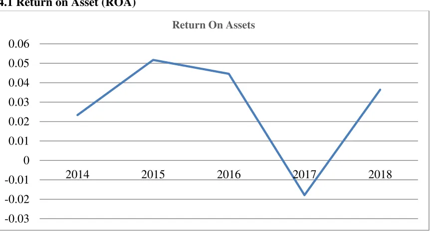
According to My Accounting Course, the return on assets also known as return on total assets, is a profitability ratio that measures the net income produced by total asset during a period by comparing net income to the average total assets. The propose of ROA is to measure how efficiently a company can manage assets to produce profits during a period. Figure 1 shows the return on assets or ROA from 2014 to 2018. The ROA in 2014 is 0.0234 and drastically rising to 0.0517 in 2015, but fall to 0.0446 in 2016. In 2017, ROA continues drop to -0.0179 however it rises to 0.036 in 2018.

The mean for ROA in these five years shows 0.0276 based on the descriptive statistics, it demonstrates that every 1 dollar that GM invest can get back 20%. The highest ROA is 0.0517 in 2015 is more than the average ROA, it means that GM can get back 5.17% in every 1 dollar they invest. In 2017 shows the lowest ROA -0.0179 which is lower than average ROA, whereby GM get a financial loss on that year. The standard deviation for ROA among these five years is 0.0275.

-0.03 -0.02 -0.01 0 0.01 0.02 0.03 0.04 0.05 0.06

2014 2015 2016 2017 2018

4.2 Current Ratio

Figure 2

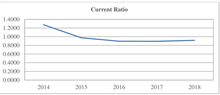
The formula of the current ratio is current assets divided by current liability, this is one of the liquidity ratios. The purpose of calculating the current ratio is to measure the ability of a company to pay back short term obligations. Figure 2 shows the current ratio within 5 years, from 2014 to 2018. The trend of current assets declines rapidly and continue to maintain at that level. In 2014, the current ratio of GM is 2.1737 and slightly decline to 0.9746 in 2015. It continues decline to 0.8946 in 2016 and meet the lowest current ratio in 2017 which is 0.8941.

The mean of the current ratio is 0.9905 according to the descriptive statistics. Every dollar of current liability has $0.9905 in current assets. In 2014 GM makes the highest current ratio which is 1.2737 and the lowest is in 2017 (0.8941). The standard deviation of current ratio is 0.1617 within these five years.

0.0000 0.2000 0.4000 0.6000 0.8000 1.0000 1.2000 1.4000

2014 2015 2016 2017 2018

4.3 Average Collection Period

Figure 3

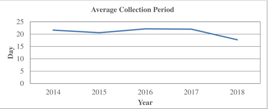
The formula of Average Collection Period is 365 days divided by average receivable turnover ratio, while the formula of the average receivable turnover ratio is net credit sales divided by average accounts receivable. This ratio is used to determine how quickly that credit purchase is collected. A lower average collection period is generally more favorable than a higher average collection period. The average collection period of 2014 is 22 days and it drops to 21 days in 2015. However in 2016 it rises to 22 days and maintain its until 2017, but it declines to 18 days in the following years.

From table X, it show that GM is efficiency in collect back all the bill from the majority customer. This is because the average collection period between these five years is 21 days, it also can be defined as GM need around 21days to collected back its debt. The highest average collection period is 22 days in 2014 while the lowest is 18 days in 2018. The lower collection is better because it means that lower credit risk and company can faster to collect back their debt. The standard deviation of the average collection period between 2014 until 2018 is 1.8371.

0 5 10 15 20 25

2014 2015 2016 2017 2018

Day

Year

4.4 Operating Margin

Figure 4

Operating Margin is to determine how much profit a company makes on a dollar sales. The method is calculation is using operating income divided by sales net sales. Figure 4 displays the value of the operating margin from 2014 to 2018. The lowest value of operating margin within these five years is .0099, its rise to 0.0376 in the following years. In 2016 operating margin continue increase to 0.0582 and hit the highest value in 2017 which is 0.0595, but it drops to 0.0302 in 2018.

The average the operating margin from 2014 to 2018 is 0.0391. The higher the operating margin the higher operating earnings example in 2017 every dollar of sales of GM can make $ 0.0595 operating earnings. The standard deviation of operating margin is .0207.

4.5 Gross Domestic Product (GDP)

Figure 5

0.0000 0.0200 0.0400 0.0600 0.0800

2014 2015 2016 2017 2018

Operating Margin

0 0.5 1 1.5 2 2.5 3 3.5

2014 2015 2016 2017 2018

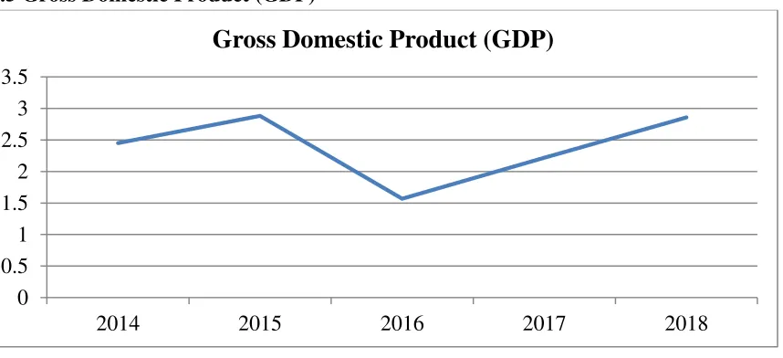
Gross Domestic Product (GDP) is monetary to measure the final goods and services produced in a specific time period. The growth of GDP will directly increase the demand for money because people will get more money to make the transaction necessary to purchase the new GDP. However, when GDP is slowing down or negative it will cause unemployment rate increase and decrease profit of the business. The figure shows that trend of GDP within these five years is fluctuate. GPD in 2014 is 2.4520 and increases to 2.8809 in the following years. However, it drops to 1.5672 in 2016, fortunately, it rises to 2.217 in 2017 and continues increases to 2.857 in 2018.

The mean of GDP within these five years is 2.3948. In 2015 GDP hit the highest value which is 2.8809 and it also above the average of a value. It can defined as America’s economy is healthy. While in 2016 it achieves the lowest GDP value which is 1.5672 and it is below than the average value. The standard deviation within these five years is 0.5408.

4.6 Inflation

Figure 6

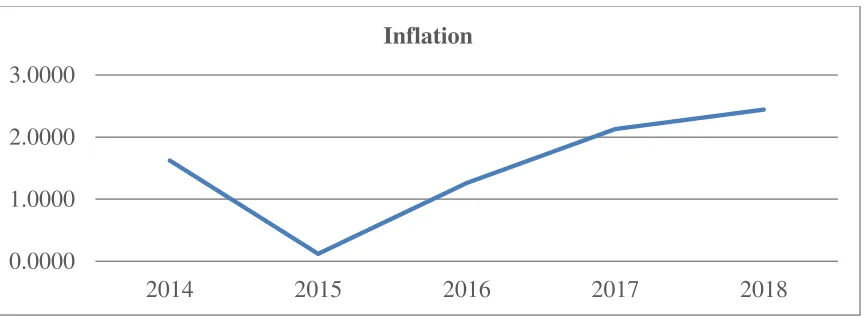
The inflation rate is to measure the average of average price level of a basket of selected goods and services in an economy increase over a while. An increase in the inflation rate directly increases the cost of living people and their living quality because they have to spend more time on working to support the family. The inflation rate of America in 2014 is 1.6222 and falls to 0.1186 in the following year. However, in 2016 it rises rapidly to 1.2616 and it continue increase to 2.1301 and 2.4426 in 2017 and 2018 respectively.

The average of inflation is from 2014 to 2018 is 1.51502. The inflation peaked at 2.4426 in 2018 within these five years, while the lowest inflation rate is in 2015 which is 0.1186 and it is below the average of inflation. The standard deviation for inflation is 0.9034.

0.0000 1.0000 2.0000 3.0000

2014 2015 2016 2017 2018

4.7 Exchange rate

Figure 7

Exchange rate is the different value between two country’s currency. The trend of exchange rate within these five years shows stable. In 2014 the exchange rate of America is 1.33 but it decline to 1.11 in the following years and it maintain until 2016. However it increase in 2017 which is 1.13 and it continue rise to 1.18 in 2018. The average of the exchange rate from 2014 to 2018 is 1.172, and the standard deviation is 0.0928. Peak of the exchange rate within these five years is in 2014 which is 1.33 and it is above the average rate, while the lowest rate is in 2015 and 2016 which is 1.11.

4.8 Interest rate

Figure 8

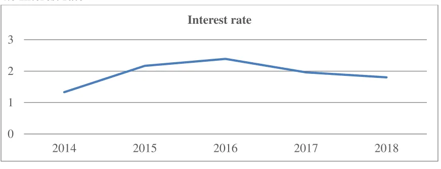
Interest rate is the amount change by lender for use of asset, the rate is depend on the lender. The trend of the interest rate in America from 2014 to 2018 shows rise and fall. In 2014 the interest rate show in figure 8 is 1.33 and it is the lowest rate within this five years. However, it rise rapid in 2015 which is 2.17, and it continue increase to the peak within these five years which is 2.39 in 2016. In 2017 it drop to 1.96, and continue drop

1 1.1 1.2 1.3 1.4

2014 2015 2016 2017 2018

Exchange rate

0 1 2 3

2014 2015 2016 2017 2018

to 1.8 in the following years. The average of interest rate within these five years is 1.93 and the standard deviation is 0.4022.

4.9 Descriptive Statistics

Descriptive Statistics

Variables (constant) Mean Std. Deviation N

Current Ratio .990503447315735 .161685589884879 5

ROA .027632095655830 .027536433090056 5

Quick Ratio 832760909526126 .131260811553008 5

Average-Collection Period 20.813508282372340 1.837113604585282 5

Debt to Income 22.937105888230610 14.204262269627957 5

Operational Ratio .980901397168703 .044515998133121 5

Operating Margin 039093145557299 .020702998038407 5

GDP 2.394819200000000 . 540762342867641 5

Inflation Rate 1.500 .8916 5

Interest Rate 1.9300 .40218 5

Exchange Rate 1.1720 .09284 5

STDV .70639700 .150308183 5

Unemployment Rate 4.940 .8792 5

Index .800 .0000 5

Descriptive Statistics is a summary statics of a collection of data and information and then analyse it. The propose of descriptive statistic is to summarize a sample, rather then use the data to learn about the population. The ROA for mean and standard deviation of General motor is 0.276 and 0.276 respectively. The mean of current ratio is 0.991 while standard deviation is 0.162. The average of quick ratio is 0.823 and standard deviation is 0.131. The average collection period for GM is 21 days while standard deviation is 1.837. Debt to income’s mean is 22.937 and the standard deviation is 14.204. The average of operational ratio and operating margin is 0.981 and 0.0391 respectively, while the standard deviation is 0.0445 and 0.207 respectively. Inflation rate, exchange rate, GDP, standard deviation, CGI, interest rate and unemployment rate are positive mean and standard deviation.

Correlation

Variables CR ROA QR ACP DTI OR OM GDP INF IR ER STDV UR CGI

Pearson CR 1.000 .029 .984 .191 .875 .546 -.805 .201 -.096 -.811 .918 .675 .853 .

Correlation ROA .029 1.000 -.012 -.342 .005 .498 -2.60 .161 -.580 .307 -.121 .325 .187 .

QR .984 -.012 1.000 .140 .924 .418 -.854 .145 .063 -.857 .968 .656 .775 .

ACP .191 -.342 .140 1.000 -.229 -.173 .352 -.705 -.291 .166 -.018 -.555 .536 .

DTI .875 .005 .924 -.229 1.0000 .384 -.940 .380 .280 -.942 .975 .813 .505 .

OR .546 .498 .418 -.173 .384 1.000 -.654 .686 -.692 -.284 .290 .750 .598 .

OM -.850 -.260 -.854 .352 -.940 -.654 1.000 -.579 -.006 .832 -.863 -.949 -.548 .

GDP .201 .161 .145 -.705 .380 .686 -.579 1.000 -.104 -.418 .206 .799 -.055 .

INF -.096 -.580 .063 -.291 .280 -.692 -.006 -.104 1.000 -.409 .293 -.064 -.520 .

IR -.811 .307 -.857 .166 -.942 -.284 .832 -.418 -.409 1.000 -.941 -.726 -.402 .

ER .918 -.121 .968 -.018 .975 .290 -.863 .206 .293 -.941 1.000 .682 .593 .

STDV .675 .325 .656 -.555 .813 .750 -.949 .799 -.064 -.726 .682 1.000 .369 .

UR .853 .187 .775 .536 .505 .598 -.548 -.055 -.520 -.402 .593 .369 1.000 .

CGI . . . 1.000

Sig. CR . .481 .001 .379 .026 .171 .034 .373 .439 .048 .014 .106 .033 .000

(1-tailed) ROA .481 . .492 .287 .497 .197 .336 .398 .153 .307 .423 .297 .382 .000

QR .001 .492 . .411 .012 .242 .033 .408 .460 .032 .003 .114 .062 .000

ACP .379 .287 .411 . .355 .390 .281 .092 .317 .395 .489 .166 .176 .000

DTI .026 .497 .012 .355 . .261 .009 .264 .324 .008 .002 .047 .193 .000

OR .171 .197 .242 .390 .261 . .116 .101 .098 .321 .318 .072 .143 .000

OM .034 .336 .033 .281 .009 .116 . .153 .496 .040 .030 .007 .170 .000

GDP .373 .398 .408 .092 .264 .101 .153 . .434 .242 .370 .052 .465 .000

INF .439 .153 .460 .317 .324 .098 .496 .434 . .247 .316 .459 .185 .000

IR .048 .07 .032 .395 .008 .321 .040 .242 .247 . .009 .083 .251 .000

ER .014 .423 .003 .489 .002 .318 .030 .370 .316 .009 . .103 .146 .000

STDV .106 .297 .114 .166 .047 .072 .007 .052 .459 .083 .103 . .271 .000

UR .033 .382 .062 .176 .193 .143 .170 .465 .185 .251 .146 .271 . .000

CGI .000 .000 .000 .000 .000 .000 .000 .000 .000 .000 .000 .000 .000 -

N CR 5 5 5 5 5 5 5 5 5 5 5 5 5 5

ROA 5 5 5 5 5 5 5 5 5 5 5 5 5 5

QR 5 5 5 5 5 5 5 5 5 5 5 5 5 5

ACP 5 5 5 5 5 5 5 5 5 5 5 5 5 5

DTI 5 5 5 5 5 5 5 5 5 5 5 5 5 5

OR 5 5 5 5 5 5 5 5 5 5 5 5 5 5

OM 5 5 5 5 5 5 5 5 5 5 5 5 5 5

GDP 5 5 5 5 5 5 5 5 5 5 5 5 5 5

INF 5 5 5 5 5 5 5 5 5 5 5 5 5 5

IR 5 5 5 5 5 5 5 5 5 5 5 5 5 5

ER 5 5 5 5 5 5 5 5 5 5 5 5 5 5

STDV 5 5 5 5 5 5 5 5 5 5 5 5 5 5

UR 5 5 5 5 5 5 5 5 5 5 5 5 5 5

Correlation is analysis show a connection or relationship between two thing or variable.

Table 1 demonstrate how the dependent variable (ROA) reacts with the independent

variable (quick ratio, current ratio, average collection period, operating margin,

operational ratio, exchange rate, GDP, inflation and interest rate). + sign means that have

a positive relationship, it also can be defined as the two variable will increase or decrease

together. However – sign is showing a negative relationship, means that when one

variable increase the other one will decrease.

According to table 1, current assets shows a high positive correlation which is 1. ROA

(0.029), quick ratio (0.984), average collection period (0.191), debt to income (0.875),

operational ratio (0.546), GDP (0.201), Exchange rate (0.918), standard deviation (0.675)

and unemployment rate (0.853) obtain positive correlation. However operating margin

(-0.850), Inflation rate (-0.096), Interest rate (-0.811) shows a negetive correlation

Significance means how they are truly connected, and the number must not more than

0.10. It divided into three-level, the first level means which is correlated with significance

and the number should less than 0.10. The second level also known as two stars is the

number should less than 0.05 means that is moderate significance with correlated. The

last level is the most significantly correlated variable and it is three stars.

According to correlation above, it demonstrate quick ratio (0.001), debt to income (0.026),

operating margin (0.034), interest rate (0.048), exchange rate (0.014) and unemployment

rate (0.033) is significance variable with current ratio, since the value is below 0.1.

However quick ratio is the most significance because the value is 0.001 and is the

smallest value. ROA (0.481), average collection period (0.379), operational ratio (0.171),

GDP (0.373), Inflation rate (0.439) and STDV (0.106) is belong to not significant value

because the value is over 0.1.

4.11 Model Summary

Model Summaryb

Model R R Square Adjusted R Square Std. Error of the Estimate Durbn-Wastson

1 .984a .969 .958 .033120352845925 2.016

ANOVAa

Model Sum of Square df Mean Square F Sig.

1 Regression .101 1 .101 92.326 .002b

Residual .003 3 .001

Total .105 4

a. Dependent Variable: Current Ratio

b. Predictors: (Constant), Quick Ratio

From the table we notice that the adjusted R square of model summary is 0.958 At the

same time, the sum of squares for regression and residual of ANOVA is 0.101 and 0.003

respectively. Thus, the mean square of regression and residual is 0.101 and 0.001

respectively. From these two table, it shows that quick ratio has significant connection

with current ratio, the movement of quick ratio will effect on the current ratio. The

liquidity of GM will effect by the quick ratio.

4.12 Coefficients

Coefficientsa

Model

Unstandardized Coefficients

Standardized Coefficients

95.0% Confidence Interval for B

Collinearity Statistics

B Std. Error Beta t Sig Lower

Bound

Upper Bound

Tolerance VIF

1 (Constant) -.019 .106 -.179 .869 -.357 .319

QR 1.212 .126 .984 .9609 .002 . 811 1.614 1.000 1.000

a. Dependent Variable : Current Ratio

The quick ratio stated that 1.212for confidence interval of B from the table above. In the

other hand, the dependent variable or constant variable is current ratio is recorded as

-0.019, it also can defined as it is the positive relationship between constant variable with

4.13 Rasiduals Statistics

Residuals Statisticsa

Minimum Maximum Mean Std. Deviation N

Predicted Value .89669573307 1.2731302976 .99050344731 .15912105972 5

Residual -.03061985783 .04644212499 .00000000000 .02868306694 5

Std. Predicted Value

-.590 1.776 .000 1.00 5

Std. Residual -.925 1.402 .000 .866 5

a. Dependent Variables : Current Ratio

The table above show forcast the value of general motor based on the dependent variable

(current ratio) is 0.992 while the standard deviation residual, residual and standard

5.0 CONCLUSION

5.1 Introduction

The study aims is to find out the internal and external factor affect performance in

General Motor Company from 2014 to 2018. Internal factor has been selected is current

ratio, quick ratio, average collection period, operational ratio and operating marginal

while the external factor has been included in this study is GDP, exchange rate and

interest rate.

5.2 Discussion on Result

Generally the liquidity of General Motor Company has a significant relationship between

current ratio with quick ratio, debt to income, operating margin, interest rate, exchange

rate and unemployment rate. For instant, the loss of bankruptcy of a company can cause

by a failure of corporate governance. This can been notice by the descriptive analysis

section. Thus the principle of corporate governance must be aware by the management

team and the board of director. Besides, based on table one the most significance

independent variable is quick ratio. Quick ratio is one of the internal factors shows most

significance variable because it has the lowest value which is 0.001.

5.3 Limitation

The limitation in this study is only five years General Motor Company’s annual report to

be investigated in this study which is from 2014 to 2018 and no comparison with other

companies. Directly it causes the limitation of data especially in calculating coefficient

and model summary in this report since only 5 years of data can be collected.

5.4 Recommendations

Based on this study has been dine, General Motors Company shows the current ratio

between these five years is continuing decline. It means that GM should increase their

assets and don’t hold too much debt, so it can increase the current ratio. The higher

current ratio can ensure the company have enough fund to cover all operating expenses

and also can decrease liquidity risk. By manage better liquidity in a company, the profit

and revenue will increase because profit has a positive relationship with liquidity. So that

REFERENCE

Core, J. E., Holthausen, R. W., & Larcker, D. F. (1999). Corporate governance, chief

executive officer compensation, and firm performance. Journal of financial economics, 51(3), 371-406.,

https://www.sciencedirect.com/science/article/pii/S0304405X98000580

Claessens, S. (2006). Corporate governance and development. The World bank research observer, 21(1), 91-122, from

https://academic.oup.com/wbro/article/21/1/91/1725521

Barakat, A., Ashby, S., Fenn, P., & Bryce, C. (2019). Operational risk and reputation in

financial institutions: Does media tone make a difference?. Journal of Banking & Finance, 98, 1-24, from

https://www.sciencedirect.com/science/article/pii/S0378426618302310

Jarrow, R. A. (2008). Operational risk. Journal of Banking & Finance, 32(5), 870-879, from

https://www.sciencedirect.com/science/article/pii/S0378426607002671

Ali, S. S. (2004, February). Islamic modes of finance and associated liquidity risks.

In conference on Monetary Sector in Iran: Structure, Performance & Challenging Issues, February, Tehran, Iran, from

http://www.sbp.org.pk/departments/ibd/lecture_6_islamic_modes_finance_liquidit

y.pdf

Dowd, K. (2007). Measuring market risk. John Wiley & Sons, from

https://books.google.com.my/books?hl=en&lr=&id=wL7hwpuTa9sC&oi=fnd&pg

=PR5&dq=market+risk+&ots=b_2zfIjdLF&sig=LdUgEA0jZSSni5Kw1D241KMI

n-M&redir_esc=y#v=onepage&q=market%20risk&f=false

Zhu, Q., Sarkis, J., & Lai, K. H. (2007). Green supply chain management: pressures,

https://scihub.tw/https://www.sciencedirect.com/science/article/pii/S09291199080

00242?via%3Dihub#

Year ROA Current Ratio

Quick Ratio

Average-Collection Period

Debt To Income

Operational Ratio

2014 0.023370996 1.2737 1.0659 21.6346 45.3399 1.0099

2015 0.051715931 0.9746 0.7813 20.5714 15.7409 1.0425

2016 0.044554693 0.8946 0.7650 22.1266 11.3350 0.9418

2017 -0.017882314 0.8941 0.7554 22.0183 13.6425 0.9405

2018 0.036401172 0.9156 0.7962 17.7165 28.6272 0.9698

Year Operating Margin

GDP Inflation Interest Rate

Exchange Rate

STDV Unemployment rate

Index

2014 0.0099 2.45 1.60 1.33 1.33 0.859777 6.2 0.8

2015 0.0376 2.88 0.10 2.17 1.11 0.771492 5.3 0.8

2016 0.0582 1.57 1.30 2.39 1.11 0.529465 4.9 0.8

2017 0.0595 2.22 2.10 1.96 1.13 0.562257 4.4 0.8