Modeling and forecasting inflation in Philippines using ARIMA models

Munich Personal RePEc Archive

Modeling and forecasting inflation in

Philippines using ARIMA models

NYONI, THABANI

UNIVERSITY OF ZIMBABWE

25 February 2019

Online at

https://mpra.ub.uni-muenchen.de/92429/

Modeling and Forecasting Inflation in Philippines using ARIMA models

Nyoni, Thabani Department of Economics

University of Zimbabwe Harare, Zimbabwe

Email: nyonithabani35@gmail.com

ABSTRACT

This research uses annual time series data on inflation rates in the Philippines from 1960 to 2017, to model and forecast inflation using ARIMA models. Diagnostic tests indicate that P is I(1). The study presents the ARIMA (1, 1, 3). The diagnostic tests further imply that the presented optimal ARIMA (1, 1, 3) model is stable and acceptable for predicting inflation in the Philippines. The results of the study apparently show that P will fall down from 5.6% in 2018 to approximately 0.3% in 2027. The Bangko Sentral ng Pilipinas is expected to continue implementing it inflation targeting policy framework since it proves to work well for the economy.

Key Words: Forecasting, Inflation, Philippines

JEL Codes: C53, E31, E37, E47

INTRODUCTION

Inflation is the sustained increase in the general level of prices and services over time (Blanchard, 2000). The negative effects of inflation are widely recognized (Fenira, 2014). Inflation is one of the central terms in macroeconomics (Enke & Mehdiyev, 2014) as it harms the stability of the acquisition power of the national currency, affects economic growth because investment projects become riskier, distorts consuming and saving decisions, causes unequal income distribution and also results in difficulties in financial intervention (Hurtado et al, 2013). The monetary authorities of a large number of countries recognize that price stability, that is, an environment of low and stable inflation rate, is the main contribution that monetary policy can give to economic growth (Allon, 2015).

In the case of Philippines, price stability is the ultimate objective of monetary policy under the inflation targeting (IT) framework which was adopted in 2002 (Allon, 2015) and such a dynamic change was to be complimented by the ability to forecast the future path of inflation in the Philippines. To avoid adjusting policy and models by not using an inflation rate prediction can result in imprecise investment and saving decisions, potentially leading to economic instability (Enke & Mehdiyev, 2014). Thus, in support of the new 2002 IT framework by the Bangko Sentral ng Pilipinas, modeling and forecasting inflation has become compulsory. In this study, we seek to model and forecast inflation in Philippines using ARIMA models.

LITERATURE REVIEW

Kock & Terasvirta (2013) forecasted Finnish consumer price inflation using Artificial Neural Network models with a data set ranging over the period March 1960 – December 2009 and established that direct forecasts are more accurate then their recursive counterparts. Allon (2015) forecasted inflation in Philippines using ARIMA models and basically established that ARIMA models were suitable for predicting inflation in the Philippines and that one-to-two months ahead forecasts from these models could be used as initial estimates to inform or initialize structural models. Kharimah et al (2015) analyzed the CPI in Malaysia using ARIMA models with a data set ranging over the period January 2009 to December 2013 and revealed that the ARIMA (1, 1, 0) was the best model to forecast CPI in Malaysia. Nyoni (2018k) studied inflation in Zimbabwe using GARCH models with a data set ranging over the period July 2009 to July 2018 and established that there is evidence of volatility persistence for Zimbabwe’s monthly inflation data. Nyoni (2018n) modeled inflation in Kenya using ARIMA and GARCH models and relied on annual time series data over the period 1960 – 2017 and found out that the ARIMA (2, 2, 1) model, the ARIMA (1, 2, 0) model and the AR (1) – GARCH (1, 1) model are good models that can be used to forecast inflation in Kenya. Nyoni & Nathaniel (2019), based on ARMA, ARIMA and GARCH models; studied inflation in Nigeria using time series data on inflation rates from 1960 to 2016 and found out that the ARMA (1, 0, 2) model is the best model for forecasting inflation rates in Nigeria.

MATERIALS & METHODS

One of the methods that are commonly used for forecasting time series data is the Autoregressive Integrated Moving Average (ARIMA) (Box & Jenkins, 1976; Brocwell & Davis, 2002; Chatfield, 2004; Wei, 2006; Cryer & Chan, 2008). For the purpose of forecasting inflation rate in Philippines, ARIMA models were specified and estimated. If the sequence ∆dPt satisfies an

ARMA (p, q) process; then the sequence of Pt also satisfies the ARIMA (p, d, q) process such

that:

∆𝑑_𝑃

𝑡 = ∑ 𝛽𝑖∆𝑑𝑃𝑡−𝑖+ 𝑝

𝑖=1

∑ 𝛼𝑖𝜇𝑡−𝑖 𝑞

𝑖=1

+ 𝜇𝑡… … … . … … … … . … … . [1]

which we can also re – write as:

∆𝑑_𝑃

𝑡 = ∑ 𝛽𝑖∆𝑑𝐿𝑖𝑃𝑡 𝑝

𝑖=1

+ ∑ 𝛼𝑖𝐿𝑖𝜇𝑡 𝑞

𝑖=1

where ∆ is the difference operator, vector β ϵⱤp and ɑ ϵⱤq.

The Box – Jenkins Methodology

The first step towards model selection is to difference the series in order to achieve stationarity. Once this process is over, the researcher will then examine the correlogram in order to decide on the appropriate orders of the AR and MA components. It is important to highlight the fact that this procedure (of choosing the AR and MA components) is biased towards the use of personal judgement because there are no clear – cut rules on how to decide on the appropriate AR and MA components. Therefore, experience plays a pivotal role in this regard. The next step is the estimation of the tentative model, after which diagnostic testing shall follow. Diagnostic checking is usually done by generating the set of residuals and testing whether they satisfy the characteristics of a white noise process. If not, there would be need for model re – specification and repetition of the same process; this time from the second stage. The process may go on and on until an appropriate model is identified (Nyoni, 2018).

Data Collection

This study is based on a data set of annual rates of inflation in the Philippines (PhINF or simply P) ranging over the period 1960 – 2017. All the data was adapted from the World Bank online database.

Diagnostic Tests & Model Evaluation

Stationarity Tests: Graphical Analysis

Figure 1

The Correlogram in Levels

0 5 10 15 20 25 30 35 40 45 50 55

Autocorrelation function for PhINF ***, **, * indicate significance at the 1%, 5%, 10% levels. Table 1

LAG ACF PACF Q-stat. [p-value]

1 0.3703 *** 0.3703 *** 8.3702 [0.004] 2 0.0487 -0.1024 8.5179 [0.014] 3 0.2309 * 0.2915 ** 11.8908 [0.008] 4 0.2619 ** 0.0815 16.3119 [0.003] 5 0.2060 0.1311 19.0972 [0.002] 6 0.1710 0.0456 21.0533 [0.002] 7 0.1973 0.1006 23.7088 [0.001] 8 0.0735 -0.1169 24.0848 [0.002] 9 0.0392 0.0074 24.1939 [0.004] 10 0.3234 ** 0.2817 ** 31.7743 [0.000] 11 0.1549 -0.1590 33.5503 [0.000]

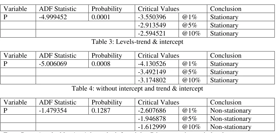
The ADF Test in Levels

Table 2: Levels-intercept

Variable ADF Statistic Probability Critical Values Conclusion P -4.999452 0.0001 -3.550396 @1% Stationary

-2.913549 @5% Stationary -2.594521 @10% Stationary Table 3: Levels-trend & intercept

Variable ADF Statistic Probability Critical Values Conclusion P -5.006069 0.0008 -4.130526 @1% Stationary

-3.492149 @5% Stationary -3.174802 @10% Stationary Table 4: without intercept and trend & intercept

Variable ADF Statistic Probability Critical Values Conclusion P -1.479354 0.1287 -2.607686 @1% Non-stationary

-1.946878 @5% Non-stationary -1.612999 @10% Non-stationary From figure 1 and tables 1 – 4, it can be inferred that P is non-stationary in levels.

Autocorrelation function for d_PhINF ***, **, * indicate significance at the 1%, 5%, 10% levels.

Table 5

LAG ACF PACF Q-stat. [p-value]

1 -0.2516 * -0.2516 * 3.8020 [0.051] 2 -0.4012 *** -0.4959 *** 13.6434 [0.001] 3 0.1245 -0.2142 14.6083 [0.002] 4 0.0710 -0.2287 * 14.9281 [0.005] 5 -0.0214 -0.1304 14.9578 [0.011] 6 -0.0447 -0.1655 15.0895 [0.020] 7 0.1202 0.0538 16.0617 [0.025] 8 -0.0749 -0.0669 16.4467 [0.036] 9 -0.2512 * -0.3312 ** 20.8663 [0.013] 10 0.3682 *** 0.1195 30.5669 [0.001] 11 0.0435 0.0208 30.7054 [0.001]

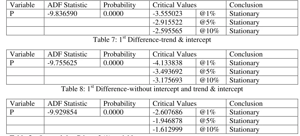
ADF Test in 1st Differences

Table 6: 1st Difference-intercept

Variable ADF Statistic Probability Critical Values Conclusion P -9.836590 0.0000 -3.555023 @1% Stationary

-2.915522 @5% Stationary -2.595565 @10% Stationary Table 7: 1st Difference-trend & intercept

Variable ADF Statistic Probability Critical Values Conclusion P -9.755625 0.0000 -4.133838 @1% Stationary

-3.493692 @5% Stationary -3.175693 @10% Stationary Table 8: 1st Difference-without intercept and trend & intercept Variable ADF Statistic Probability Critical Values Conclusion P -9.929854 0.0000 -2.607686 @1% Stationary

Evaluation of ARIMA models (without a constant)

Table 9

Model AIC ME MAE RMSE MAPE ARIMA (1, 1, 1) 402.2285 -0.09846 4.6289 7.7679 95.478 ARIMA (1, 1, 0) 417.289 -0.035411 5.296 9.0783 107.45 ARIMA (0, 1, 1) 401.632 -0.10523 4.6827 7.8583 97.245 ARIMA (2, 1, 1) 398.5884 -0.12047 4.56 7.3791 78.495 ARIMA (1, 1, 2) 400.0143 -0.10957 4.5765 7.482 84.095 ARIMA (2, 1, 2) 400.2586 -0.11921 4.5398 7.3586 77.676 ARIMA (1, 1, 3) 397.3587 -0.17487 4.6835 7.2097 83.941 ARIMA (1, 1, 4) 399.1992 -0.17072 4.6311 7.1957 83.041 ARIMA (3, 1, 1) 400.417 -0.11889 4.561 7.3688 78.171 A model with a lower AIC value is better than the one with a higher AIC value (Nyoni, 2018). The study will only consider the AIC as the criteria for choosing the best model for predicting inflation in Philippines. Hence, the ARIMA (1, 1, 3) model is finally chosen.

95% Confidence Ellipse & 95% 95% Marginal Intervals

Figure 2 [AR (1) & MA (1) components]

Figure 3 [AR (1) & MA (2) components]

-2.2 -2 -1.8 -1.6 -1.4 -1.2 -1 -0.8 -0.6 -0.4

0.2 0.3 0.4 0.5 0.6 0.7 0.8 0.9 1 1.1 0.692, -1.36

phi_1

Figure 4 [AR (1) & MA (3) components]

-0.8 -0.6 -0.4 -0.2 0 0.2 0.4 0.6 0.8

0.2 0.3 0.4 0.5 0.6 0.7 0.8 0.9 1 1.1 0.692, -0.0359

phi_1

95% confidence ellipse and 95% marginal intervals

0 0.1 0.2 0.3 0.4 0.5 0.6 0.7 0.8 0.9 1

0.2 0.3 0.4 0.5 0.6 0.7 0.8 0.9 1 1.1 0.692, 0.516

phi_1

Figure 5 [MA (1) & MA (2) components]

Figure 6 [MA (1) & MA (3) components]

-0.8 -0.6 -0.4 -0.2 0 0.2 0.4 0.6 0.8

-2.2 -2 -1.8 -1.6 -1.4 -1.2 -1 -0.8 -0.6 -0.4 -1.36, -0.0359

theta_1

95% confidence ellipse and 95% marginal intervals

0 0.1 0.2 0.3 0.4 0.5 0.6 0.7 0.8 0.9 1

-2.2 -2 -1.8 -1.6 -1.4 -1.2 -1 -0.8 -0.6 -0.4 -1.36, 0.516

theta_1

Figure 7 [MA (2) & MA (3) components]

Figures 2 – 7 indicate that the accuracy of our forecast is satisfactory since it falls within the 95% confidence interval.

Residual & Stability Tests

ADF Tests of the Residuals of the ARIMA (1, 1, 3) Model

Table 10: Levels-intercept

Variable ADF Statistic Probability Critical Values Conclusion Rt -7.370142 0.0000 -3.555023 @1% Stationary

-2.915522 @5% Stationary -2.595565 @10% Stationary Table 11: Levels-trend & intercept

Variable ADF Statistic Probability Critical Values Conclusion Rt -7.448820 0.0000 -4.133838 @1% Stationary

-3.493692 @5% Stationary

0 0.1 0.2 0.3 0.4 0.5 0.6 0.7 0.8 0.9 1

-0.8 -0.6 -0.4 -0.2 0 0.2 0.4 0.6 0.8

-0.0359, 0.516

theta_2

-3.175693 @10% Stationary Table 12: without intercept and trend & intercept

Variable ADF Statistic Probability Critical Values Conclusion Rt -7.428858 0.0000 -2.607686 @1% Stationary

-1.946878 @5% Stationary -1.612999 @10% Stationary

Tables 10, 11 and 12 show that the residuals of the ARIMA (1, 1, 3) model are stationary and hence the ARIMA (1, 1, 3) model is suitable for forecasting inflation in Philippines.

Stability Test of the ARIMA (1, 1, 3) Model

Figure 8

Since the corresponding inverse roots of the characteristic polynomial lie in the unit circle, it illustrates that the chosen ARIMA (1, 1, 3) model is stable and suitable for predicting inflation in Philippines over the period under study.

FINDINGS

Descriptive Statistics

Table 13 Description Statistic

Mean 8.7448

Median 6.4

Minimum 0.7

-1.5 -1.0 -0.5 0.0 0.5 1.0 1.5

-1.5 -1.0 -0.5 0.0 0.5 1.0 1.5 AR roots

MA roots

Maximum 50.3 Standard deviation 8.4039 Skewness 2.7432 Excess kurtosis 9.6451

As shown above, the mean is positive, i.e. 8.7448%. The minimum is 0.7% and the maximum is 50.3%. The skewness is 2.7432 and the most striking characteristic is that it is positive, indicating that the inflation series is positively skewed and non-symmetric. Excess kurtosis was found to be 9.6451; implying that the inflation series is not normally distributed.

Results Presentation1

Table 14

ARIMA (1, 1, 3) Model:

∆𝑃𝑡−1= 0.691749∆𝑃𝑡−1−1.35594𝜇𝑡−1− 0.0359261𝜇𝑡−2+ 0.516476𝜇𝑡−3… … … . [3]

P: (0.0000) (0.0000) (0.8951) (0.0048) S. E: (0.157) (0.3025) (0.2724) (0.1831)

Variable Coefficient Standard Error z p-value AR (1) 0.691749 0.157026 4.405 0.0000*** MA (1) -1.35594 0.302517 -4.482 0.0000*** MA (2) -0.0359261 0.272426 -0.1319 0.8951 MA (3) 0.516476 0.183146 2.82 0.0048***

Predicted Annual Inflation in Philippines

Table 15

Year Prediction Std. Error 95% Confidence Interval 2018 5.6 6.98 -8.1 - 19.3

2019 5.6 7.36 -8.8 - 20.0 2020 3.9 7.45 -10.7 - 18.5 2021 2.7 7.45 -11.9 - 17.3 2022 1.9 7.51 -12.8 - 16.6 2023 1.3 7.66 -13.7 - 16.3 2024 0.9 7.89 -14.5 - 16.4 2025 0.7 8.20 -15.4 - 16.7

1

2026 0.5 8.54 -16.3 - 17.2 2027 0.3 8.90 -17.1 - 17.8

Table 15, with a forecast range from 2018 – 2027; clearly show that inflation in the Philippines is projected to fall from 5.6% in 2018 to approximately 0.3% in 2027, ceteris paribus. This could be attributed to the success of the Bangko Sentral ng Pilipinas’s inflation-targeting (IT) framework.

CONCLUSION

The ARIMA model was employed to investigate annual inflation rates in Philippines from 1960 to 2017. The ARIMA (1, 1, 3) model, which was found to be the best model, was also found to be stable. Based on the results, policy makers in the Philippines should continue to engage proper economic policies in order to suppress persistent inflationary pressures in the economy. In this regard, the Bangko Sentral ng Pilipinas is encouraged to stick to its mandated inflation-targeting framework because it has proved to be fruitful over the study period.

REFERENCES

[1] Allon, J. C. S (2015). Forecasting Inflation: A Disaggregated Approach Using ARIMA Models, Research Department, Bangko Sentral ng Pilipinas.

[2] Blanchard, O (2000). Macroeconomics, 2nd Edition, Prentice Hall, New York.

[3] Box, G. E. P & Jenkins, G. M (1976). Time Series Analysis: Forecasting and Control,

Holden Day, San Francisco.

[4] Brocwell, P. J & Davis, R. A (2002). Introduction to Time Series and Forecasting,

Springer, New York.

[5] Buelens, C (2012). Inflation modeling and the crisis: assessing the impact on the performance of different forecasting models and methods, European Commission, Economic Paper No. 451.

[6] Chatfield, C (2004). The Analysis of Time Series: An Introduction, 6th Edition, Chapman & Hall, New York.

[7] Cryer, J. D & Chan, K. S (2008). Time Series Analysis with Application in R, Springer, New York.

[8] Enke, D & Mehdiyev, N (2014). A Hybrid Neuro-Fuzzy Model to Forecast Inflation,

Procedia Computer Science, 36 (2014): 254 – 260.

[10] Hector, A & Valle, S (2002). Inflation forecasts with ARIMA and Vector Autoregressive models in Guatemala, Economic Research Department, Banco de Guatemala.

[11] Hurtado, C., Luis, J., Fregoso, C & Hector, J (2013). Forecasting Mexican Inflation Using Neural Networks, International Conference on Electronics, Communications and Computing, 2013: 32 – 35.

[12] Kharimah, F., Usman, M., Elfaki, W & Elfaki, F. A. M (2015). Time Series Modelling and Forecasting of the Consumer Price Bandar Lampung, Sci. Int (Lahore)., 27 (5): 4119 – 4624.

[13] King, M (2005). Monetary Policy: Practice Ahead of Theory, Bank of England.

[14] Kock, A. B & Terasvirta, T (2013). Forecasting the Finnish Consumer Price Inflation using Artificial Network Models and Three Automated Model Section Techniques, Finnish Economic Papers, 26 (1): 13 – 24.

[15] Mcnelis, P. D & Mcadam, P (2004). Forecasting Inflation with Think Models and Neural Networks, Working Paper Series, European Central Bank.

[16] Nyoni, T & Nathaniel, S. P (2019). Modeling Rates of Inflation in Nigeria: An Application of ARMA, ARIMA and GARCH models, Munich University Library – Munich Personal RePEc Archive (MPRA), Paper No. 91351.

[17] Nyoni, T (2018). Modeling and Forecasting Inflation in Kenya: Recent Insights from ARIMA and GARCH analysis, Dimorian Review, 5 (6): 16 – 40.

[18] Nyoni, T (2018). Modeling and Forecasting Inflation in Zimbabwe: a Generalized Autoregressive Conditionally Heteroskedastic (GARCH) approach, Munich University Library – Munich Personal RePEc Archive (MPRA), Paper No. 88132.

[19] Nyoni, T. (2018). Box – Jenkins ARIMA Approach to Predicting net FDI inflows in Zimbabwe, Munich University Library – Munich Personal RePEc Archive (MPRA), Paper No. 87737.

[20] Wei, W. S (2006). Time Series Analysis: Univariate and Multivariate Methods, 2nd Edition, Pearson Education Inc, Canada.