Group Sparse CNNs for Question Classification with Answer Sets

Proceedings of the 55th Annual Meeting of the Association for Computational Linguistics (Short Papers), pages 335–340 Vancouver, Canada, July 30 - August 4, 2017. c2017 Association for Computational Linguistics

Proceedings of the 55th Annual Meeting of the Association for Computational Linguistics (Short Papers), pages 335–340 Vancouver, Canada, July 30 - August 4, 2017. c2017 Association for Computational Linguistics

Group Sparse CNNs for Question Classification with Answer Sets

Mingbo Ma Liang Huang

School of EECS Oregon State University Corvallis, OR 97331, USA {mam,liang.huang}@oregonstate.edu

Bing Xiang Bowen Zhou

IBM Watson Group T. J. Watson Research Center Yorktown Heights, NY 10598, USA

{bingxia,zhou}@us.ibm.com

Abstract

Question classification is an important task with wide applications. However, tra-ditional techniques treat questions as gen-eral sentences, ignoring the corresponding answer data. In order to consider answer information into question modeling, we first introduce novel group sparse autoen-coders which refine question representa-tion by utilizing group informarepresenta-tion in the answer set. We then propose novel group sparse CNNs which naturally learn ques-tion representaques-tion with respect to their answers by implanting group sparse au-toencoders into traditional CNNs. The proposed model significantly outperform strong baselines on four datasets.

1 Introduction

Question classification has applications in many domains ranging from question answering to di-alog systems, and has been increasingly popular in recent years. Several recent efforts (Kim,2014; Kalchbrenner et al., 2014;Ma et al., 2015) treat questions as general sentences and employ Con-volutional Neural Networks (CNNs) to achieve re-markably strong performance in the TREC ques-tion classificaques-tion task.

We argue, however, that those general sentence modeling frameworks neglect two unique proper-ties of question classification. First, different from the flat and coarse categories in most sentence classification tasks (i.e. sentimental classification), question classes often have a hierarchical struc-ture such as those from the New York State DMV FAQ1_{(see Fig.1). Another unique aspect of} ques-tion classificaques-tion is the well prepared answers for each question or question category. These answer 1_{Crawled fromhttp://nysdmv.custhelp.com/app/home.} This data and our code will be athttp://github.com/cosmmb.

1: Driver License/Permit/Non-Driver ID

a:Apply for original (49 questions)

b:Renew or replace (24 questions)

...

2: Vehicle Registrations and Insurance

a:Buy, sell, or transfer a vehicle (22 questions) b:Reg. and title requirements (42 questions) ...

3: Driving Record / Tickets / Points

...

Figure 1: Examples from NYDMV FAQs. There are 8 top-level categories, 47 sub-categories, and 537 questions (among them 388 areunique; many questions fall into multiple categories).

sets generally cover a larger vocabulary (than the questions themselves) and provide richer informa-tion for each class. We believe there is a great po-tential to enhance question representation with ex-tra information from corresponding answer sets.

To exploit the hierarchical and overlapping structures in question categories and extra infor-mation from answer sets, we consider dictionary learning (Cand`es and Wakin, 2008; Rubinstein et al.,2010) which is a common approach for rep-resenting samples from many correlated groups with external information. This learning pro-cedure first builds a dictionary with a series of grouped bases. These bases can be initialized ran-domly or from external data (from the answer set in our case) and optimized during training through Sparse Group Lasso (SGL) (Simon et al.,2013).

To apply dictionary learning to CNN, we first develop a neural version of SGL, Group Sparse Autoencoders (GSAs), which to the best of our knowledge, is the first full neural model with group sparse constraints. The encoding matrix of GSA (like the dictionary in SGL) is grouped into different categories. The bases in different groups can be either initialized randomly or by

the sentences in corresponding answer categories. Each question sentence will be reconstructed by a few bases within a few groups. GSA can use either linear or nonlinear encoding or decoding while SGL is restricted to be linear. Eventually, to model questions with sparsity, we further pro-pose novel Group Sparse Convolutional Neural Networks(GSCNNs) by implanting the GSA onto CNNs, essentially enforcing group sparsity be-tween the convolutional and classification layers. This framework is a jointly trained neural model to learn question representation with group sparse constraints from both question and answer sets.

2 Group Sparse Autoencoders

2.1 Sparse Autoencoders

Autoencoder (Bengio et al.,2007) is an unsuper-vised neural network which learns the hidden rep-resentations from data. When the number of hid-den units is large (e.g., bigger than input dimen-sion), we can still discover the underlying struc-ture by imposing sparsity constraints, using sparse autoencoders (SAE) (Ng,2011):

Jsparse(ρ) =J +α

s

X

j=1

KL(ρ_kρˆj) (1)

whereJ is the autoencoder reconstruction loss,ρ

is the desired sparsity level which is small, and thus Jsparse(ρ) is the sparsity-constrained version

of loss J. Here α is the weight of the sparsity

penalty term defined below:

KL(ρ_kρˆj) =ρlog ρ

ˆ

ρj

+ (1₋ρ) log 1−ρ 1₋ρˆj (2)

where

ˆ

ρj = 1 m

m

X

i=1

hi_j

represents the average activation of hidden unitj

overmexamples (SAE assumes the input features

are correlated).

As described above, SAE has a similar objec-tive to traditional sparse coding which tries to find sparse representations for input samples. Besides applying simple sparse constraints to the network, group sparse constraints is also desired when the class categories are structured and overlapped. In-spired by group sparse lasso (Yuan and Lin,2006) and sparse group lasso (Simon et al., 2013), we propose a novel architecture below.

2.2 Group Sparse Autoencoders

Group Sparse Autoencoder (GSA), unlike SAE, categorizes the weight matrix into different groups. For a given input, GSA reconstructs the input signal with the activations from only a few groups. Similar to the average activation ρˆj for

sparse autoencoders, GSA defines each grouped average activation for the hidden layer as follows:

ˆ

ηp=

1

mg m

X

i=1

g

X

l=1

khi_p,lk2 (3)

wheregrepresents the size of each group, andηˆj

first sums up all the activations withinpth group,

then computes the average pth group respond

across different samples’ hidden activations. Similar to Eq. 2, we also use KL divergence to measure the difference between estimated intra-group activation and global intra-group sparsity:

KL(η_kηˆp) =ηlog η

ˆ

ηp

+ (1₋η) log 1−η 1₋ηˆp (4)

whereGis the number of groups. Then the

objec-tive function of GSA is:

Jgroupsparse(ρ, η) =J+α

s

X

j=1

KL(ρ_kρˆj)

+β G

X

p=1

KL(ηkηˆp)

(5)

where ρ and η are constant scalars which are

our target sparsity and group-sparsity levels, resp. When α is set to zero, GSA only considers the

structure between difference groups. When β is

set to zero, GSA is reduced to SAE.

2.3 Visualizing Group Sparse Autoencoders

In order to have a better understanding of GSA, we use the MNIST dataset to visualize GSA’s internal parameters. Fig. 2 and Fig. 3 illustrate the pro-jection matrix and the corresponding hidden acti-vations. We use 10,000 training samples. We set the size of the hidden layer to 500 with 10 groups. Fig.2(a) visualizes the input image for hand writ-ten digit0.

(a)

1 2 3 4 5 6 7 8 9 10

(b) (c)

Figure 2: The input figure with hand written digit0is shown in (a). Figure (b) is the visualization of trained projection matrixWon MNIST dataset. Different rows represent different groups ofWin Eq.5.

For each group, we only show the first 15 (out of 50) bases. The red numbers on the left side are the indices of 10 different groups. Figure (c) is the projection matrix from basic autoencoders.

1 | 2 | 3 | 4 | 5 | 6 | 7 | 8 | 9 | 10

(a) (b)

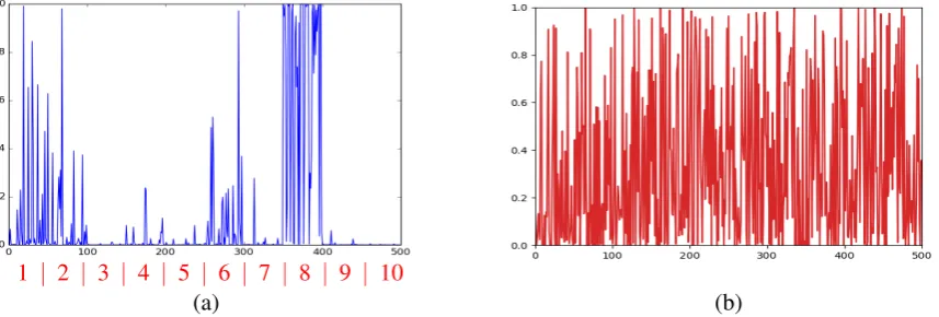
Figure 3: (a): the hidden activationshfor the input image in Fig.2(a). The red numbers corresponds to

the index in Fig.2(b). (b): the hidden activationshfor the same input image from basic autoencoders.

Fig.3(a) shows the hidden activations with re-spect to the input image of digit 0. The patterns of the 10th _{row in Fig.2(b) are very similar to digit}

1 which is very different from digit 0 in shape.

Therefore, there is no activation in group 10 in Fig.3(a). The majority of hidden layer activations are in groups 1, 2, 6 and 8, with group 8 being the most significant. When compared to the projection matrix visualization in Fig.2(b), these results are reasonable since the 8th _{row has the most similar}

patterns of digit 0. However, we could not find any meaningful pattern from the hidden activations of basic autoencoder as shown in Fig.3(b).

GSA could be directly applied to small image data (e.g. MINIST dataset) for pre-training. How-ever, in tasks which prefer dense semantic rep-resentations (e.g. sentence classification), we still need CNNs to learn the sentence representation automatically. In order to combine advantages from GSA and CNNs, we propose Group Sparse

Convolutional Neural Networks below.

3 Group Sparse CNNs

CNNs were first proposed by (LeCun et al.,1995) in computer vision and adapted to NLP by ( Col-lobert et al., 2011). Recently, many CNN-based techniques have achieved great successes in sen-tence modeling and classification (Kim, 2014; Kalchbrenner et al.,2014).

Following sequential CNNs, one dimensional convolutions operate the convolution kernel in se-quential order xi,j = xi ⊕ xi+1 ⊕ · · · ⊕ xi+j,

wherexi ∈Rerepresents theedimensional word

representation for the i-th word in the sentence,

and ⊕ is the concatenation operator. Therefore

xi,j refers to concatenated word vector from the i-th word to the(i+j)-th word in sentence.

A convolution operates a filter w ∈ Rn×e _to

Any interesting places to visit in Lisbon

…

…

…

… …

…

N

fi

lte

rs

(

Pooling Feed

into NN

Group Sparse Auto-Encoder

Convolutional Layer

W

z

h

z

W,

W

b

(

·

,

b

)

(

·

)

h

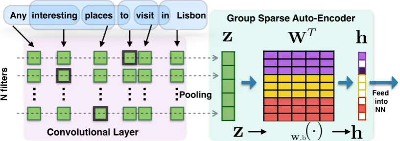
Figure 4: Group Sparse CNN. We add an extra dictionary learning layer between sentence representation

zand the final classification layer.Wis the projection matrix (functions as a dictionary) that convertsz

to the group sparse representationh(Eq.5). Different colors in the projection matrix represent different

groups. We showW|instead ofWfor presentation purposes. Darker colors inh mean larger values

and white means zero.

functionσ to produce a new feature. The filterw

is applied to each word in the sentence, generating the feature mapa = [a1, a2,· · · , aL]whereLis

the sentence length. We then useˆa= max_{a_}to

represent the entire feature map after max-pooling. In order to capture different aspects of patterns, CNNs usually randomly initialize a set of filters with different sizes and values. Each filter will generate a feature as described above. To take all the features generated by N different filters into

count, we use z = [ ˆa1,· · ·,aˆN]as the final

rep-resentation. In conventional CNNs, thisz will be directly fed into classifiers after the sentence rep-resentation is obtained, e.g. fully connected neural networks (Kim,2014). There is no easy way for CNNs to explore the possible hidden representa-tions with underlaying structures.

In order to exploit these structures, we pro-pose Group Sparse Convolutional Neural Net-works (GSCNNs) by placing one extra layer be-tween the convolutional and the classification lay-ers. This extra layer mimics the functionality of GSA from Section 2. Shown in Fig.4, after the conventional convolutional layer, we get the fea-ture mapzfor each sentence. In stead of directly

feeding it into a fully connected neural network for classification, we enforce the group sparse con-straint on z in a way similar to the group sparse

constraints on hidden layer in GSA from Sec. 2. Then, we use the sparse hidden representation h

in Eq.5as the new sentence representation, which is then fed into a fully connected neural network for classification. The parametersWin Eq.5will

also be fine tunned during the last step.

Different ways of initializing the projection ma-trix in Eq.5can be summarized below:

• Random Initialization: When there is no an-swer corpus available, we first randomly ini-tializeN vectors to represent the group

infor-mation from the answer set. Then we clus-ter theseN vectors into Gcategories withg

centroids for each category. These centroids from different categories will be the initial-ized bases for projection matrix W which will be learned during training.

• Initialization from Questions: Instead of using random initialized vectors, we can also use question sentences for initializing the projection matrix when the answer set is not available. We need to pre-train the sentences with CNNs to get the sentence representa-tion. We then selectG largest categories in

terms of number of question sentences. Then we getg centroids from each category byk

-means. We concatenate theseG×gvectors

to form the projection matrix.

• Initialization from Answers: This is the most ideal case. We follow the same proce-dure as above, with the only difference being using the answer sentences in place of ques-tion sentences to pre-train the CNNs.

4 Experiments

suit-Datasets Ct Cs Ndata Ntest Nans Multi-label TREC 6 50 5952 500 - No INSURANCE - 319 1580 303 2176 Yes

DMV 8 47 388 50 2859 Yes YAHOOAns 27 678 8871 3027 10365 No Table 1: Summary of datasets. Ct and Cs are

the numbers of top-level and sub- categories, resp.

Ndata, Ntest, Nans are the sizes of data set, test set, and answer set, resp. Multilabel means each question can belong to multiple categories.

able datasets which are publicly available. We collected two datasets ourselves and also used two other well-known ones. These datasets are summarized in Table 1. INSURANCE is a pri-vate dataset we collected from a car insurance company’s website. Each question is classified into 319 classes with corresponding answer data. All questions which belong to the same category share the same answers. The DMV dataset is col-lected from New York State the DMV’s FAQ web-site. The YAHOO Ans dataset is only a subset of the original publicly available YAHOOAnswers dataset (Fleming et al.,2012;Shah and Pomerantz, 2010). Though not very suitable for our frame-work, we still included the frequently used TREC dataset (factoid question type classification) for comparison.

We only compare our model’s performance with CNNs for two following reasons: we consider our “group sparsity” as a modification to the general CNNs for grouped feature selection. This idea is orthogonal to any other CNN-based models and can be easily applied to them; in addition, as dis-cussed in Sec.1, we did not find any other model in comparison with solving question classification tasks with answer sets.

There is crucial difference between the INSUR -ANCEand DMV datasets on one hand and the YA -HOO set on the other. In INSURANCEand DMV, all questions in the same (sub)category share the same answers, whereas YAHOOprovides individ-ual answers to each question.

For multi-label classification (INSURANCE and DMV), we replace the softmax layer in CNNs with a sigmoid layer which predicts each category independently while softmax is not.

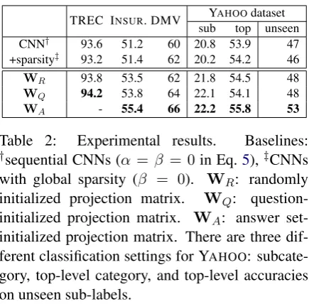
All experimental results are summarized in Ta-ble 2. The improvements are substantial for IN -SURANCE and DMV, but not as significant for YAHOO and TREC. One reason for this is the

TREC INSUR. DMV _subYAHOO_{top unseen}dataset

CNN† _{93.6 51.2 60 20.8 53.9 47}

+sparsity‡ _{93.2 51.4 62 20.2 54.2 46} WR 93.8 53.5 62 21.8 54.5 48

WQ 94.2 53.8 64 22.1 54.1 48

WA - 55.4 66 22.2 55.8 53 Table 2: Experimental results. Baselines: †_{sequential CNNs (α = β = 0in Eq.5),}‡_CNNs with global sparsity (β = 0). WR: randomly

initialized projection matrix. WQ:

question-initialized projection matrix. WA: answer

set-initialized projection matrix. There are three dif-ferent classification settings for YAHOO: subcate-gory, top-level catesubcate-gory, and top-level accuracies on unseen sub-labels.

questions in YAHOO/TREC are shorter, which makes the group information harder to encode. Another reason is that each question in YA -HOO/TREC has a single label, and thus can not fully benefit from group sparse properties.

Besides the conventional classification tasks, we also test our proposed model on an unseen-label case. In these experiments, there are a few sub-category labels that are not included in the training data. However, we still hope that our model could still return the correct parent cate-gory for these unseen subcategories at test time. In the testing set of YAHOOdataset, we randomly add 100 questions whose subcategory labels are unseen in training set. The classification results of YAHOO-unseen in Table 2 are obtained by map-ping the predicted subcategories back to top-level categories. The improvements are substantial due to the group information encoding.

5 Conclusions

In order to better represent question sentences with answer sets and group structure, we first presented a novel GSA framework, a neural version of dic-tionary learning. We then proposed group sparse convolutional neural networks by embedding GSA into CNNs, which result in significantly better question classification over strong baselines. Acknowledgment

References

Yoshua Bengio, Pascal Lamblin, Dan Popovici, and Hugo Larochelle. 2007. Greedy layer-wise training of deep networks. InAdvances in Neural Informa-tion Processing Systems 19.

Emmanuel J. Cand`es and Michael B. Wakin. 2008.

An Introduction To Compressive Sampling. In

Signal Processing Magazine, IEEE. volume 25.

http://dx.doi.org/10.1109/msp.2007.914731. R. Collobert, J. Weston, L. Bottou, M. Karlen,

K. Kavukcuoglu, and P. Kuksa. 2011. Natural lan-guage processing (almost) from scratch. InJournal of Machine Learning Research. volume 12, pages 2493–2537.

Simon Fleming, Dan Chalmers, and Ian Wakeman. 2012. A deniable and efficient question and answer service over ad hoc social networks. InInformation Retrieval.

Nal Kalchbrenner, Edward Grefenstette, and Phil Blun-som. 2014. A convolutional neural network for modelling sentences. In Proceedings of the 52nd Annual Meeting of the Association for Computa-tional Linguistics. Association for Computational Linguistics.

Yoon Kim. 2014. Convolutional neural networks for sentence classification. InProceedings of the 2014 Conference on Empirical Methods in Natural Lan-guage Processing (EMNLP). Association for Com-putational Linguistics, Doha, Qatar, pages 1746– 1751.http://www.aclweb.org/anthology/D14-1181.

Y. LeCun, L. Jackel, L. Bottou, A. Brunot, C. Cortes, J. Denker, H. Drucker, I. Guyon, U. Mller, E. Sckinger, P. Simard, and V. Vapnik. 1995. Com-parison of learning algorithms for handwritten digit recognition. In International Conference on Artifi-cial Neural Networks. pages 53–60.

Mingbo Ma, Liang Huang, Bing Xiang, and Bowen Zhou. 2015. Dependency-based convolutional neu-ral networks for sentence embedding. In Proceed-ings of ACL 2015.

Andrew Ng. 2011. Sparse autoencoder. InCS294A Lecture notes. Stanford University, page 72. R. Rubinstein, A. M. Bruckstein, and M. Elad. 2010.

Dictionaries for sparse representation modeling. In

Neural Computation.

Chirag Shah and Jefferey Pomerantz. 2010. Evaluating and predicting answer quality in community qa. In

Proceedings of the 33rd International ACM SIGIR Conference on Research and Development in Infor-mation Retrieval. ACM, New York, NY, USA. Noah Simon, Jerome Friedman, Trevor Hastie, and

Rob Tibshirani. 2013. A sparse-group lasso. In

Journal of Computational and Graphical Statistics. Ming Yuan and Yi Lin. 2006. Model selection and

es-timation in regression with grouped variables. In