J. Range Manage.
55: 235-241 May 2002
Evaluation of
atechnique for measuring canopy volume of shrubs
MARK S. THORNE, QUENTIN D. SKINNER, MICHAEL A. SMITH, J. DANIEL RODGERS, WILLIAM A.
LAYCOCK, AND SULE A. CEREKCI
Authors are Graduate Research Assistant, Department of Rangeland Ecosystem Science, Colorado State University, Fort Collins, Cob, Professors, Assistant Professor, and Professor Emeritus, Department of Renewable Resources, University of Wyoming, Laramie, Wyo., and Project Engineer, Ministry of Agriculture and Rural Affairs, Eastern Anatolia Watershed Rehabilitation Project, Turkey. At the time of research, the senior author was a Graduate Research Assistant, Department of Renewable Resources, University of Wyoming, Laramie, Wyo.
Abstract
Cover methods quantify vegetative communities in only 2 dimensions. The addition of height measurements to cover data, resulting in canopy volume estimates, provide a more practical level of description for shrub communities. We evaluated a tech- nique to estimate canopy volume of shrubs that used a formula [2/3tH (A12 x B/2)] derived from the basic ellipsoid volume for- mula. Objectives of this study were to determine if there were significant differences among means of repeated observations on sample units: (1) among observers; (2) within observers; and (3) between sample periods when using this technique. At 2 locations in Wyoming, 10 planeleaf willow (Salix planifolia var. planifolia Pursh) plants along each of 5 randomly established transects were sampled during 2 consecutive periods by 4 observers.
Differences among observers were significant at both sites (P <
0.05). However, within observer variation between sample peri- ods was not significant (P > 0.05) at either site. Mean canopy vol- ume did not vary significantly (P > 0.05) between sample periods when averaged across observers. Estimated sample sizes ranged between 2 and 31 transects depending on the desired sampling precision and confidence level. The average time per transect among all observers decreased from 13 minutes (SD = 3.7) in sample period 1 to 9 minutes (SD =1.3) in sample period 2. Using this method, managers can better describe and monitor trends in the structural diversity of shrub communities. This canopy vol- ume technique can be applied with minimal training and is pre- cise, efficient, and repeatable.
Key Words: willow (Salix spp.), measurement variability, sam- pling techniques, sample size
Resumen
Los metodos de cobertura cuantifican las comunidades vegeta- tivas en solo 2 dimensiones. La adicion de mediciones de altura a los datos de cobertura resultan en estimaciones del volumen de la copa y proveen un nivel mas practico de descripcion de las comunidades de arbustos. Evaluamos una tecnica para estimar el volumen de copa de los arbustos que utiliza una formula [
2/3tH (A/2 x B/2)] derivada de la formula basica para calcular el volumen de un elipsoide. Los objetivos de este estudio fueron determinar si hubo diferencias significativas entre las medias de observaciones repetidas en unidades de muestreo: (1) entre observadores; (2) dentro de observadores y (3) entre periodos de muestreo cuando se utiliza esta tecnica. En 2 localidades de Wyoming, 10 plantas de "Planeleaf willow" (Salix planifolia var.
planifolia Pursh), situadas a to largo de cada uno de 5 transecto establecidos aleatoriamente, se muestrearon por 4 observadores durante 2 periodos consecutivos. Las diferencias entre obser- vadores fueron significativas en ambos sitios (P < 0.05). Sin embargo, la variacion dentro de observadores entre los periodos de muestro no fue significativa (P > 0.05) en ningun sitio.
Cuando la media del volumen de la copa se promedio entre observadores esta no vario significativamente (P > 0.05) entre los periodos de muestreo. Los tamanos de muestra estimados van- anon entre 2 y 31 transecto, dependiendo de la precision de muestreo y nivel de confianza deseados. El tiempo promedio por transecto entre todos los observadores disminuyo de 13 minutos (DS = 3.7) en el periodo de muestreo 1 a 9 minutos (DS =1.3) en el periodo de muestreo 2. Usando este metodo los manejadores pueden describir y monitorear mejor las tendencias en la diversi- dad estructural de las comunidades de arbustos. Esta tecnica de volumen de copa puede ser aplicada con un entrenamiento mini- mo y es precisa, eficiente y repetible.
Early researchers realized that temporal changes in plant cover were often a reflection of management practices and developed appropriate techniques to quantify those changes (Nelson 1930, Pickford and Stewart 1935, Bauer 1936, Parker 1951, Cooper 1957, Daubenmire 1959). Other investigators noted that plant
Research was funded in part by the Wyoming Water Resources Center, the Hyatt Ranch, the Pitchfork Ranch, the WesMar Grazing Management Trust Fund, and the SRM Hyatt Trust. Authors wish to thank Dr. Robert S. Cochran of the Statistics Department at the University of Wyoming for assistance in statistical analyses. We would also like to thank Dr. J. Brummer and 2 anonymous reviewers for their insightful comments and suggestions on drafts of this manuscript.
Manuscript accepted 22 Aug. Ol.
cover estimates varied between methods, observers, and vegeta- tion types (Smith 1944, Johnston 1957, Heady et al. 1959, Kinsinger et al. 1960, Fisser 1961). Despite problems with preci- sion, repeatability, and efficiency, these methods remain in com- mon use.
Cover methods quantify vegetative communities in only 2
dimensions. Daubenmire (1968) noted that the omission of the vertical dimension was the largest limitation to cover data. He also pointed out that, since height was a structural parameter, it could be used to determine and compare dominance of plant species in a community. Zamora (1981) modified Daubenmire's
JOURNAL OF RANGE MANAGEMENT 55(3) May 235
(1959) quadrat frame with the addition of a vertical dimension and suggested that it could be used to quantify canopy volume in shrub communities. Recently, Myers (1989) suggested that the addition of height measurements might be a more practical level of description for riparian shrub communities. In addition, canopy volume estimates have been used for pre- dicting biomass or current-year twig pro- duction of shrubs (Lyon 1968, Peek 1970, Rittenhouse and Sneva 1977, Uresk et al.
1977, Bryant and Kothmann 1979, Creamer 1991).
More recently, several investigators have used canopy volume to quantify other attributes of shrub communities. For example, Taylor (1986) used canopy vol- ume to define nesting habitat suitability for passerine birds in willow (Salix spp.) communities along the Blitzen River in Oregon. Manoukian (1994) used canopy volume to describe seasonal changes in Montana willow communities subjected to wildlife and livestock herbivory.
Although prior studies have focused on estimating plant volume, all used different measures of the volume components.
Likewise, a variety of mathematical for- mulas have been used to calculate volume.
Therefore, comparing canopy volume esti- mates among different studies and man- agement programs is difficult. Since canopy volume is an important attribute in shrub communities and its estimation is becoming more common, it may be appro- priate to standardize an approach to mea- sure it. It would also be convenient to use a mathematical formula that is elastic in its ability to absorb a wide range of canopy shapes. Several factors could define the usefulness of a standard method of mea- suring canopy volume such as ease of application, efficiency, precision, and repeatability.
Ease of application is related to the sim- plicity of the methodology. Efficiency is a function of the time it takes to make a pre- cise and repeatable estimate where as, pre- cision and repeatability of an estimate are controlled by the inherent variation in the vegetative community and error caused by the method and observer. Error imposed by the method and variation in the vegeta- tive community are uncontrollable. Since vegetative communities are the object of study, controlling this source of variation in the estimate is only desirable for sources not related to the community or temporal factors of interest. Conversely, error in accuracy imposed by a method
designed to measure vegetative attributes is always undesirable. If a method (assum- ing no observer error) continuously over- or underestimates an attribute of interest, then it is a less desirable technique.
Canopy Volume Formula
In estimating plant canopy volumes, the largest source of methodological error lies in the volume formula. Lyon (1968), Peek (1970), Creamer (1991), and Manoukian (1994) used mathematically equivalent formulas for an elliptical cylinder to esti- mate canopy volume of different shrub species. The elliptical cylinder formula, V
= t(H)[Major axis/2 x Minor axisl21, where H is the plant height, assumes right angles at both the base and crest of the shape for which volume is being estimat- ed. This formula may overestimate plant canopy volume because it does not inte- grate changing radial distances along the vertical axis of the plant. Shrub canopy volume estimates have also been calculat- ed using the rectangular volume formula (H x W x L) reported by Uresk et al.
(1977). Since plants tend to be bounded by a spherical or elliptical form, the rectangu- lar volume formula may overestimate plant canopy volume by a factor of r.
Conversely, the conical volume formula reported by Bryant and Kothmann (1978), V = (t r2 H)13, where H is the plant height, may underestimate canopy vol- ume. The conical formula assumes that the junction of the central vertical axis and the
Basic ellipsoid volume formula
V=413itABC
widest radial plane is a right angle, and that the radial distances are equal across all horizontal axes. Most plants, even when severely hedged, would not meet these requirements, and averaging unequal radial distances of the horizontal axes forces the plant into a contrived canopy shape thus altering the estimate of volume.
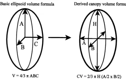
The ellipsoid volume formula [2I3tH (A12 x B12)] used in this study is not sub- ject to the limitations described above (Fig. 1). Changing radial distances along the vertical axes are accounted for within the formula. The formula is elastic and accurately accommodates a wide range of plant shapes and sizes. Specifically, the formula can absorb plant shapes that are non-concentric about the horizontal axis and either compressed or elongated along the vertical axis. Thorne (1998) found that the ellipsoid volume formula was sensitive to changes in plant dimensions over time.
Importantly, growth, utilization, and twig death do not affect the application of the formula. Because the ellipsoid form
"adjusts" to the varying sizes and shapes of plants, consecutive observations closely reflect what has been gained or lost over time.
The purpose of this study was to describe and evaluate the efficiency, preci- sion, and repeatability of a technique to estimate canopy volume of shrubs. The objectives were to determine if there were significant differences among means of repeated observations on sample units: (1)
Derived canopy volume formula
CV=213irH(AI2xBl2)
Fig. 1. The canopy volume formula used in this study was derived from the basic ellipsoid volume formula. In the canopy volume (CV) formula, H is substituted for A and is the height of the plant from the base to the top of the photosynthetically active material. Both A and B in the CV formula are diameter readings taken at 50% of the plant height across the plane of photosynthetically active material. Because height and diameter meaurements are used, it is necessary to divide the components of the basic volume formula by 2 so that volume will be properly estimated.
236 JOURNAL OF RANGE MANAGEMENT 55(3) May 2002
among observers, (2) within observers, and (3) between sample periods (means pooled across observers). Secondarily, we asked; could the variability be reduced if observers were trained and the plants were well defined and easy to distinguish?
Materials and Methods
Study Areas
This study was conducted in a planeleaf willow (Salix planifolia var. planifolia Pursh) community located on the Paintrock Grazing Allotment (Willow Swamp; 44°21 N, 107° 21' W), Paintrock District, Bighorn National Forest, Wyo. in July 1997. The allotment was approxi- mately 24 km east of Hyattville, Wyo. and ranged in elevation from 2,150 m to over 3,700 m. Annual precipitation ranged from 380 mm at the lower elevations to 1,020 mm at the higher elevations. The shrub component of Willow Swamp (elev. 2,675 m) was actually dominated by bog birch (Betula glandulosa Michx.), but a substan- tial amount of planeleaf willow was pre- sent (Meiman 1996).
A second set of observations were taken among potted planeleaf willows in August 1997 in a common garden at the Greenhouse Facility of the University of Wyoming (41°19' N, 105°35 W). All plants used in this study were established from stem cuttings of planeleaf willow collected from Willow Swamp in May 1994 for a frequency of clipping study (Thorne 1998).
The observations taken at the Willow Swamp site represented a "worst case"
scenario where observers were not trained and the plants were not easily distinguish- able. At this site, willows and bog birch grew in close proximity to each other, often with branches intertwined. In other cases, 2 or 3 separately rooted willow plants grew on the same hummock making it difficult to separate plants for the pur- pose of estimating canopy volume. The observations taken at the garden site repre- sented a "best case" scenario where the plants were easily distinguishable and the observers were more familiar with the technique. Since the plants at the garden were potted separately (i.e., 1 plant per pot) on a 1 x 2 m grid, distinguishing between plants was not a problem.
Further, the same observers were used for both sites and, in effect, had become trained at Willow Swamp for the observa- tions at the Garden site.
Experimental Design
A completely randomized, repeated measures sample design was used at both sites. At the Willow Swamp site, a base line was established from the northeast corner of a U. S. Forest Service wildlife and livestock exclosure and continued eastward for 100 m. Along the base line, 5
perpendicular sub-transects were estab- lished at random distances running south to north. From each sub-transect, one mea- surement transect was randomly estab- lished that ran east to west if the distance up the sub-transect from the base line was an even value or west to east if the value was odd. Along each of the measurement transects, 10 random distances between 0 and 35 m were selected. Pin flags were placed in the vicinity of each plant along each transect to assist in locating plants during observations. Canopy volume was estimated on the willow nearest to each pin flag along each of the 5 measurement transects.
At the Garden site, five, 10 plant transects were randomly selected from a pool of all possible 10 plant combinations among 200 potted willows. This was done to provide continuity in sampling design between the Garden and Willow Swamp sites.
At both sites, canopy volume measure- ments along the set of transects, 1 through 5, were taken twice (sample periods 1 and 2) by each of 4 observers (A, B, C, and D). Each of the 5 transects was considered an observation. Both sample periods were conducted on the same day at both the Willow Swamp and Garden sites on their respective sampling dates. To estimate technique efficiency, the amount of time for each observer to complete a transect was recorded for sample periods 1 and 2 at the Willow Swamp site.
Canopy volume components were mea- sured by taking the height and 2 diameter readings at 50% of the willow height.
Willow height was defined as the distance from the base of the mainstem to the tallest extent of photosynthetically active plant material. Diameter readings were defined as the widest extent of photosyn- thetically active plant material that inter- sected a plane passing horizontally through the plant at 50% of the plant height. The 2 diameter readings were taken at right angles to each other (one parallel and the other perpendicular to the transect line). Willow canopy volume was estimated by applying the height and 2 diameter measurements to a derivative of the basic ellipsoid volume formula,
Canopy Volume = 2I3t Height (Al2 x B12), where Height is the distance from the base of the plant to the tallest photo- synthetically active material and A and B are the diameter readings taken at 50% of plant height with B perpendicular to A (Fig. 1).
The experiment was analyzed using a
repeated measures analysis of variance (AOV) with plants as the subject, transects as the within-subject term, and observers and sample period as the between-subject factors (Vonesh and Chinchilli 1997). The model included 2- and 3-way interactions of observers, transects, and sample peri- ods. Plants and transects were random terms. Observer was tested using the tran- sect x observer interaction as the error term. Sample period was tested with the
transect x sample period error term.
Observer x sample period was tested with the error term from the transect x observer x sample period interaction. Transect x observer x sample period, observer x plant within transect, and sample period x plant within transect were tested with the resid- ual error term. Since transects were ran- domly selected, the error terms testing transect, plant within transect, transect x
observer, and transect x sample period were estimated using the appropriate expected mean squares (Dowdy and Wearden 1991, Vonesh and Chinchilli 1997). Duncan's New Multiple Range (DNMR) Test was used to compare means among and within observers and sample
periods (Duncan 1955, Dowdy and Wearden 1991) when appropriate. All mean separations were conducted with an overall a of 0.05 and 12 degrees of free- dom.
To compare the consistency and preci- sion among and within observers, coeffi- cients of variation were calculated by sam- ple period for each observer. Since the coefficient of variation is a measure of the internal variability of an estimate, differ- ences among sequential coefficient values for the same sample unit reflect a shift in the degree of observer error. Thus, smaller coefficient of variation values were inter- preted to indicate greater precision in an estimate. Consistency across sample peri- ods was considered to be explained by the degree of similarity in coefficient of varia- tion values when AOV indicated non-sig- nificance.
Sample size calculations were conduct- ed to estimate the number of 10 plant tran- sects required to achieve a sampling preci- sion (E) of ± 10, 20, or 30% of the mean
JOURNAL OF RANGE MANAGEMENT 55(3) May 237
total canopy volume of the willow popula- tion at the study sites with confidence intervals of 80, 90, or 95%. Desired sample sizes were estimated using the average coefficient of variation for each of the 4 observers estimated for sample periods 1 and 2 at each study site. The formula used to estimate sample size was: n = t2 CV2IE2 where t is the critical t-value evaluated at al2 and oc degrees of freedom; CV is the
coefficient of variation; and E is the desired sampling precision (Zamora 1981).
Results
Willow Swamp Site
At the Willow Swamp site, differences among transects, and transect x observer, observer x sample period, and transect x observer x sample period interactions were not significant (P = 0.296, 0.846, 0.151, and 0.069, respectively). Observer A's estimate of mean canopy volume increased by 19% between sample periods
1 and 2, while the coefficients of variation changed from 26 to 29%, respectively (Table 1). Conversely, estimated mean canopy volume decreased by 3, 19, and 6% between sample periods 1 and 2 for observers B, C, and D, respectively (Table 1). Coefficients of variation also increased between sample periods 1 and 2 for observers B, C, and D (Table 1).
Observers varied significantly (P = 0.009) in their estimates of canopy volume at the Willow Swamp site. However, while the average canopy volume estimat- ed by observer B was significantly differ- ent from the other observers, estimates among observers A, C, and D were not different (Table 1). The transect x sample period interaction was not significant (P = 0.493) for Willow Swamp. When mean canopy volume was pooled across observers, sample period 1 (81,043 ± 6,626 cm3 SE; n = 20) did not vary (P = 0.814) from sample period 2 (79,599 ± 7,786 cm3 SE; n = 20).
The average time to measure canopy volume along a transect decreased from sample period 1 to 2 for all observers.
Observer D had the largest decrease aver- aging 17.2 minutes (SD = 5.07) per tran- sect during sample period 1 compared to 9.3 minutes (SD = 1.3) during sample period 2. Observers A, B, and C averaged 11.1 ± 1.03, 8.4 ± 2.1, and 13.2 ± 3 min- utes per transect to measure canopy vol- ume during sample period 1, respectively.
During sample period 2, the average time per transect decreased to 9.4 ± 0.5, 7.6 ± 2.1, and 9.6 ± 0.5 minutes for observers A, B, and C, respectively. The average time per transect among all observers for sam- ple period 1 was 12.5 minutes (SD = 3.7) and decreased to 9.3 minutes (SD =1.3) in sample period 2.
Garden Site
At the garden site, differences among transects, and transect x observer, observer x sample period, and transect x observer x sample period interactions were not signif- icant (P = 0.493, 0.604, 0.06, and 0.163,
respectively). Mean canopy volume decreased between sample periods 1 and 2 by 2, 10, and 5% for observers A, B, and D, respectively (Table 2). Conversely, the estimated mean canopy volume increased by nearly 17% for observer C.
Coefficients of variation at the Garden site remained constant at 23% for observer A,
increased for observers B and D, and decreased for observer C.
Observers varied significantly (P <
0.001) in their estimate of canopy volume for the Garden site (Table 2). Mean canopy volume estimates of observers A and D were similar and significantly dif- ferent from the average volume estimates of observers B and C which were also similar. At the Garden site, the transect x sample period interaction was not signifi- cant (P = 0.854). When canopy volume estimates were pooled across observers, sample period 1 (159,187 ± 24,993 cm3 SE; n = 20) did not vary (P = 0.510) from sample period 2 (157,512 ± 21,060 cm3 SE; n= 20).
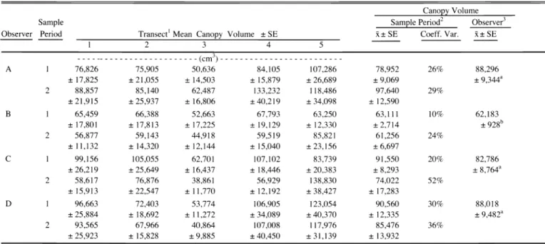
Table 1. Mean canopy volume (cm3) for each observer by transect and sample period for measurements taken at Willow Swamp, 17 Jul. 1997.
Canopy Volume
Sample Sample Period Observer3
Observer Period Transect' Mean Canopy Volume ± SE x± SE Var. SE
1 2 3 4 5
---(cm)--- 3
A 1 76,826 75,905 50,636 84,105 107,286 78,952 26% 88,296
±17,825 ±21,055 ± 14,503 ± 15,879 ± 26,689 ±9,069 ± 9,344a
2 88,857 85,140 62,487 133,232 118,486 97,640 29%
±21,915 ± 25,937 ±16,806 ±40,219 ±34,098 ± 12,590
B 1 65,459 66,388 52,663 67,793 63,250 63,111 10% 62,183
± 17,801 ± 17,813 ± 17,225 ± 19,129 ± 12,330 ±2,714 ± 928b
2 56,877 59,143 44,918 59,519 85,821 61,256 24%
±11,132 ±14,320 ±12,144 ±15,040 ±23,156 ± 6,697
C 1 99,156 105,055 62,701 107,102 83,739 91,550 20% 82,786
±26,219 ± 25,649 ± 16,437 ± 18,446 ± 20,383 ±8,293 ± 8,764a
2 58,617 76,876 38,861 56,929 138,830 74,022 52%
±15,913 ±22,547 ±11,770 ±12,192 ±38,427 ± 17,283
D 1 96,663 72,403 53,774 106,905 123,054 90,560 30% 88,018
±25,884 ± 18,692 ±11,272 ±34,089 ±40,370 ±12,335 ± 9,482a
2 93,565 67,966 40,864 107,008 117,976 85,476 36%
± 25,923 ± 15,828 ±9,885 ±40,450 ±31,139 ± 13,932
Transect mean canopy volume t standard error of the mean (cm3), n =10; within observer means at transect level were not significantly different (P > 0.05).
Sample period mean canopy volume ± standard error of the mean (cm3), n = 5 (average of 5 transects); within observer means at the sample period level were not significantly differ- ent (P > 0.05)
3Mean canopy volume ± standard error of the mean (cm3) by observer, n = 2 (average across sample periods); means among observers were significantly different (P < 0.05), likelet- tered means were not different using Duncan's New Multiple Range Test.
238 JOURNAL OF RANGE MANAGEMENT 55(3) May 2002
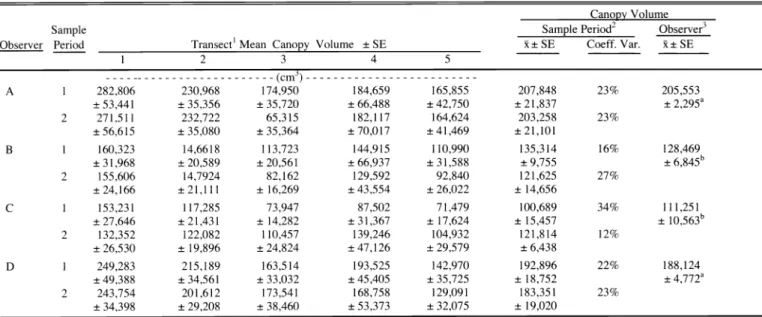
Table 2. Mean canopy volume (cm3) for each observer by transect and sample period for measurements taken at the Garden site, 29 Aug. 1997.
Canopy Volume
Sample Sample Period2 Observer3
Observer Period Transectl Mean Canopy Volume ± SE x ± SE Var. SE
1 2 3 4 5
A 1 282,806 230,968 174,950 184,659 165,855 207,848 23% 205,553
±53,441 ±35,356 ±35,720 ± 66,488 ± 42,750 ± 21,837 ± 2,295a
2 271,511 232,722 65,315 182,117 164,624 203,258 23%
± 56,615 ± 35,080 ± 35,364 ±70,017 ±41,469 ±21,101
B 1 160,323 14,6618 113,723 144,915 110,990 135,314 16% 128,469
± 31,968 t 20,589 ± 20,561 ± 66,937 ± 31,588 ± 9,755 ± 6,845b
2 155,606 14,7924 82,162 129,592 92,840 121,625 27%
± 24,166 ±21,111 ±16,269 ±43,554 ±26,022 ± 14,656
C 1 153,231 117,285 73,947 87,502 71,479 100,689 34% 111,251
± 27,646 ±21,431 ±14,282 ±31,367 ±17,624 ±15,457 ± 10,563b
2 132,352 122,082 110,457 139,246 104,932 121,814 12%
± 26,530 ±19,896 ±24,824 ±47,126 ±29,579 ±6,438
D 1 249,283 215,189 163,514 193,525 142,970 192,896 22% 188,124
± 49,388 ±34,561 ±33,032 ±45,405 ±35,725 ±18,752 ± 4,772a
2 243,754 201,612 173,541 168,758 129,091 183,351 23%
± 34,398 ± 29,208 ± 38,460 ± 53,373 ± 32,075 ± 19,020
'Transect mean canopy volume ± standard error of the mean (cm3), n =10; within observer means at transect level were not significantly different (P > 0.05).
2 Sample period mean canopy volume ± standard error of the mean (cm3), n = 5 (average of 5 transects); within observer means at the sample period level were not significantly differ- ent (P > 0.05).
MMean
canopy volume ± standard error of the mean (cm3) by observer, n = 2 (average across sample periods); means among observers were significantly different (P < 0.05), like let- tered means were not different using Duncan's New Multiple Range Test.
Sample Size
The average coefficient of variation among both sample periods for all observers was 28% (± 12.25 SD) for Willow Swamp and 22.5% (± 6.61 SD) for the Garden site. Our estimates of sample size were evaluated with the variation based on 5 transects comprised of 10
plants each. Consequently, the sample sizes reported here should be considered as the minimum estimated number of tran- sects with 10 plants each required to meet
experimental design restrictions. At Willow Swamp, sample sizes ranged between 2 and 31 transects depending on the level of desired precision and confi- dence level (Table 3). For the Garden site, the largest estimated sample size was 20 transects required to obtain an estimate within ± 10% of the population mean at the 95% confidence level (Table 3). The minimum viable number of transects esti- mated to be required at the Garden site was 2 (one transect does not provide an estimate of variability and, thus, is not a viable sample size).
ment plant, b) its photosynthetically active material, and c) where to place the mea- suring rods. Sampling error was com- pounded when several willows occurred on the same hummock together or with bog birch plants. Consequently, it was possible for an observer to mistakenly measure more or less plant, or a different plant at the second sample period. At the Garden site, these sources of observer error were controlled. Observers had gained experience from the Willow Swamp measurements and plant identifi- cation problems were eliminated.
Consistency, Precision, and Efficiency
The lack of significance in the AOV among the interaction terms at both sites
indicated that observers were consistent in
their estimates of mean canopy volume between sample periods. Observer consis- tency was also reflected by the degree of similarity in their respective canopy vol- ume estimates and coefficients of variation across sample periods. Although mean canopy volume estimates within observers remained similar, there was an increase in the coefficients of variation between sam- ple periods for all observers at Willow Swamp. While difficulty in identifying the same plant or the amount of plant mea- sured between sample periods may have contributed to these differences, fatigue may have been an important factor as well. For example, observer C became ill during the second sample period possibly
contributing to the larger difference
Discussion
At Willow Swamp, 3 of the 4 observers did not have experience with this tech- nique before taking measurements.
Training included only a brief introduction on the identification of: a) the measure-
Table 3. Estimated number of transects of 10 plants each required to achieve sampling precision (E) of ± 10, 20, and 30% of the mean total canopy volume of the willow populations at the Willow Swamp and Garden sites at confidence levels of 80, 90, and 95%.
Confidence Level
Site Sampling Precision 80% 90% 95%
Willow Swamp (CV = 28% ± 12.35)' ---(%)--- ---(Sample Size)---
±10 13 22 31
±20 4 6 8
±30 2 3 4
Garden (CV = 22.5% ± 6.61)
±10 9 14 20
±20 3 4 5
±30 12 2 3
'CV = coefficient of variation; coefficients presented in this table are the average CV of observers for both sample peri- ods at each site (n = 8).
Note that 1 transect does not provide an estimate of variability and, thus, is not a viable sample size.
JOURNAL OF RANGE MANAGEMENT 55(3) May 239