1
Extended State Dependent Parameter Modelling with a Data-Based
Mechanistic Approach to Nonlinear Model Structure Identification
David A. Mindham, Wlodzimierz Tych*, Nick A. Chappell Lancaster Environment Centre, Lancaster University Corresponding author: [email protected]
Abstract
A unified approach to Multiple and single State Dependent Parameter modelling, termed Extended State Dependent Parameters (ESDP) modelling, of nonlinear dynamic systems described by time-varying dynamic models applied to ARX or transfer-function model structures. Crucially, the approach proposes an effective model structure identification method using a novel Information Criterion (IC) taking into account model complexity in terms of the number of states involved. In ESDP, model structure involves not only the model orders, but also selection of the states driving the parameters, which effectively prevents the use of most current IC. This leads to a powerful
methodology for investigating nonlinear systems building on the Data-Based Mechanistic (DBM) philosophy of Young and expanding the applications of the existing DBM methods. The
methodologies presented are tested and demonstrated on both simulated data and on high frequency hydrological observations, showing how structure identification leads to discovery of dynamic relationships between system variables.
Keywords
Nonlinear dynamic systems, model identification, Data Based Mechanistic modelling, state-dependent parameters, hydrological modelling, information criterion
1.0 Introduction
The Data-Based Mechanistic methodology (DBM, Young, 1999a) is built on the premise that the model structure and parameters are to be determined through statistical analysis of observed data (‘data-based’) which then, along with model metrics leads to a physical interpretation of the model (‘mechanistic’).
The presented approach completes the nonlinear DBM modelling process by adding an objective identification stage to the nonlinear model selection. Multiple and single State Dependent Parameter (MSDP and SDP) modelling follows the DBM methodology by not parameterising the individual nonlinearities, however the selection of the model structure, including that of the nonlinear drivers, is the key element missing from the current method.
2
The new model structure identification procedure allows for the first time identification of nonlinear structural relationships in an objective manner using a robust and tested model form. This is
demonstrated in the paper using high frequency hydrological observations, where the output variable is thought to be affected by more than one nonlinear process.
The terminology, explanation and clarification for the above are laid out below in a logical and methodical manner designed to lead the reader first through existing SDP and MSDP methodologies, then through the process of updating and extending these methodologies into one methodology described in this paper (ESDP – Extended SDP) with useful output tools. Finally, through the process of producing a generalised Model Structure Identification (MSI) procedure to identify the structure from a given data set for the application of ESDP. The MSI procedure is generalised in that it considers - no state dependency for each parameter (linear model) and one or more state dependencies for one or more parameters (nonlinear model).
1.1 Objectives and Structure of this Paper
This paper presents three key updates and additions to the SDP and MSDP methodologies leading to their unification and generalisation (items 1,..,3), and one major development (item 4) for applying the DBM approach to model structure identification in this new setting:
1. Transition to a true state-space for parameter estimation by moving from equidistant states to arbitrary-distant states, based on the state values. The terms and context of ‘state-space’ and ‘states’ are clarified and discussed in section 1.4 and onwards. (Section 2.0) 2. Formation of multivariable parameter maps from M-dimensional state dependent
parameters for the purposes of basic model validation and more importantly, for forecasting, scenario investigation and on-line simulation of live events. (Section 2.1) 3. Use of model validation techniques to not only quantify the ability of the presented
algorithms in parameter estimation, but also to validate any models identified from the model structure identification development step below. (Section 2.2)
4. Development of a DBM approach for model structure identification (MSI) from a group of data sets for a given model type so that the data informs us which measured variables are more influential to the observed model output – importantly this methodology also considers a linear model, allowing for a ‘pure’ DBM approach. (Section 3.0)
The whole approach is then applied to a hydrological example using a dynamic model of streamflow generation, thus forming objective 5. (Section 4.0)
1.2 Applications
The methodologies presented are general and can be applied to any system as long as time-series data for all the required variables (including inputs, outputs and additional states) are available. In terms of specific environmental applications, we have evaluated the approach for data in the two applications below, and present the former in this paper:
3
• Water quality dynamics – how the dynamics of one output water quality variable (e.g., Dissolved Organic Carbon concentration) may be affected by more than one nonlinear process, related to separate effects of e.g., rainfall, soil temperature and solar radiation (Jones et al., 2014).
For clarity and in order to introduce the notation, this paper also briefly covers the progression from Transfer Function (TF) to SDP TF (for a more detailed account see Young, 2000) and MSDP TF, with the novel generalisation elements introduced. Significantly, the development of the structural identification methodology for this wide class of nonlinear models is then covered.
1.3 Background to SDP
There is extensive work on modelling input-output dynamic time-series data using Transfer
Functions (TF or equivalent Auto-Regressive with eXogenous inputs, or ARX models) where linear or approximated linear relationships are used (Ockenden and Chappell, 2011; Tych et al, 2014; Ampadu et al, 2015; Chappell et al., 2017) as well as extensions into Time Varying Parameter (TVP) TF (Gou, 1990) and further extensions into State Dependent Parameter (SDP) TF (Young et al, 2001) with latter approaches using nonlinear functional relationships between states of the system and the ARX or TF parameters.
SDP modelling assumes that the system is truly nonlinear in that the TF parameters are time varying; importantly, the rate of change of the parameters is at a rate related to the rate of change within the state variables. This is unlike the more commonly seen time varying parameter TF models, where the parameters change smoothly. Here, the parameters are functions of the input or other states of the system under study. SDP, as originally published by Young (2000) bears the assumption that each parameter is a function of one variable only, and has been successfully applied to many nonlinear systems (e.g. Young et al, 2007a; Taylor et al., 2009; McIntyre et al., 2011). However, many systems, particularly in the natural environment, are complex dynamic systems with many variables that have interlinking relationships, e.g. water quality (Jones et al., 2014), atmospheric chemistry (Seinfeld and Pandis, 2016), and climate change (Ashkenazy et al., 2003; Young and Garnier, 2006). The parameters of models describing these environmental systems, or even just their specific aspects, could be functions of more than one variable and hence the need to generalise SDP modelling into the of Multiple State Dependent Parameter (MSDP) modelling.
1.4 ARX - Transfer Function (TF) – Time Invariant and Time Varying Parameter (TVP) Issues We begin with a simple linear discrete time dynamic model with time varying parameters (ARX or equivalent TF structure (Young, 1999b)) that relates a single input variable (ut) to an output variable (yt) and can be written as a difference equation (1). Due to the time-varying character of parameters the standard backward shift TF models are not applicable.
𝑦"= −𝑎&,"𝑦"(&− ⋯ − 𝑎*,"𝑦"(*+ 𝑏-,"𝑢"(/+ 𝑏&,"𝑢"(/(&+ ⋯ + 𝑏0,"𝑢"(/(0+ 𝑒" (1) where δ is a pure time delay (measured at this stage in sampling intervals), 𝑒" is a zero mean, serially uncorrelated input with variance σ2 and Gaussian amplitude distribution. The latter (Normality)
4
Expressing (1) as a vector equation we obtain the TVP observation equation: 𝑦"= 𝒛"3𝒑"+ 𝑒" (2)
where,
𝒛"3 = [−𝑦
"(& −𝑦"(7 ⋯ −𝑦"(* 𝑢"(/ ⋯ 𝑢"(/(0]
𝒑" = 9𝑎&," 𝑎7," ⋯ 𝑎*," 𝑏-," ⋯ 𝑏0,":3
When 𝒑" changes slowly/smoothly there are methods to estimate these changes taking advantage of the smoothness assumption (see for example Dynamic Transfer Function or DARX models – Young, 2011).
However, many environmental systems can be described as complex and nonlinear, where the rates of change of the parameters vary at a rate commensurate to that of other, exogenous variables. This means the changes in 𝒑" are too rapid to apply the smoothness assumption (slow parametric changes) and so other estimation methods are required. If the parameters are varying at a rate similar to that of the rate of another system variable, then that system variable must be
incorporated into the model in some form. This leads to SDP modelling where it is assumed that each parameter is dependent on a system variable. For complex systems the number of variables could be large, for example in a streamflow generation (rainfall-runoff) system there is more to consider than just rainfall and streamflow - solar radiation (controlling evaporation), soil saturation or water table depth within a deep underlying rock aquifer, may also affect the processes in
nonlinear ways (e.g., Ockenden and Chappell, 2011; Deutscher et al., 2016). 1.5 State Dependent Parameter (SDP) Input-Output models
In (2) each of the parameters 𝒑" can be further defined as a function of identified, but in general arbitrarily chosen, independent variables treated as states 𝒔" of the same system, hence the name State Dependent Parameters. This is done in the SDP approach (Young, 2000) for a single
independent state variable.
Following Young (2000) and then Tych et al (2012), we describe the time varying model parameters (pt) using stochastic dynamic system definition, where the ith parameter (-ai for i≤n, bi-(n+1) if i>n) can be defined as a Generalised Random Walk process. Then, in the specific case of Integrated Random Walk every parameter is defined by a two-dimensional stochastic state vector xi,t = [li,t di,t]T,
where li,t and di,t are, respectively, the changing level and slope of the associated time varying
parameter (Young, 2011) model. Note that the state vector x in this context is used to formulate the estimation procedure and is not the same as the SDP vector s of states driving the parameters. These are states within different spaces – x is the state used to model and estimate the parametric change as a stochastic process, and s is a part of the SDP model.
5
estimated in an arbitrary order (k=1:N) along a trajectoryKwithin that state space (not the time sequence t). For a parameter driven by a single independent state variable (as in Young, 2000), typically the order is based upon the ascending order of the independent state.
These parameters can be then estimated recursively using a Kalman Filter (KF, Kalman 1960) and Fixed-Interval Smoothing (FIS) combination along the trajectory K resulting in the stochastic state space equation for the ith parameter (3), i = 1,…, n+m.
Variation along the trajectory in the state-space (SS) of each parameter i of the n+m model parameters is modelled as a stochastic state space model:
𝒙=> = 𝐹𝒙 =(& > + 𝐺𝜂
=(& > (3) with: 𝐹 = ⎣ ⎢ ⎢ ⎢ ⎢ ⎢
⎡1 1 & 7 0 1 1 0 0 1
⋯ & GH!
& (GH(&)!
& (GH(7)!
⋮ ⋱ ⋮
0 0 0 ⋯ 1 ⎦
⎥ ⎥ ⎥ ⎥ ⎥ ⎤
, 𝐺 = Q(G&
HR&)!
& GH!
& (GH(&)⋯ 1S
3
where, 𝐻>,=3 is a 1xn observation matrix (input variable corresponding to the ith parameter), 𝜂=(&is a (in general) q+1 dimensional vector of system disturbance, with q = 0,1,2… referring to
respectively; random walk, integrated random walk, double integrated random walk, etc. For the n+m parameter model this becomes a block-diagonal SS model of higher dimension. The observation equation for this SS is Equation 2 with parameters vector p being a subset of the above state vector xas in the original SDP approach (see e.g. Young, 2000).
The individual variance terms of 𝜂> form the state covariance matrix Q (diagonal in this case). With the univariate observation series the variance of the observation disturbance ratio of σi2 is a scalar
used to standardise the KF variance parameters (as in Young, 2011). The resulting Noise Variance Ratio (NVR) matrix – the meta-parameter of the filtering and smoothing process becomes:
𝑁𝑉𝑅 = 𝑄
𝜎7
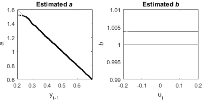
An example of a simple SDP is illustrated with a Nonlinear ARX (NARX) structure and is a forced logistic growth equation (4) similar to that found in Young (2000). In (4) and further on, s is defined as a vector variable that the parameter is dependent on, known as ‘state variable’ or ‘state’ vector.
𝑦" = 𝑎(𝒔𝒕)". 𝑦"(&+ 𝑏(1)". 𝑢"+ 𝑒" (4)
6
[image:6.595.122.474.140.314.2]standard deviations of approx. 5% of standard deviation of 𝑦". The SDP function from the Captain Toolbox (Young et al., 2007b) was used to estimate the parameters for this model (Figure 1).
Figure 1. Illustration of a simple SDP. Left hand plot, estimation of a, which is a function of yt-1. Right hand plot, estimation of b, which is a constant of 1. Light grey shows the actual values, black - the
estimated values.
To avoid any confusion in the sequel, which would be due to the estimation technique using state-space approach of the state-dependent parameters, we use 𝒔" reordered from the temporal sequence into 𝒔= along the trajectory K to denote the exogenous, independent variables affecting the input-output model parameters, and 𝒙= - the estimates of parameters sequence 𝒑= tracked by the variable step KF/FIS algorithm based on (3).
As already mentioned the SDP approach only considers one state per parameter and in more complex nonlinear systems it is likely that more than one state will influence each parameter. This leads to the extension into Multiple SDP (MSDP).
1.6 Multiple State Dependent Parameter Models
The approach taken in SDP applies to MSDP with two exceptions; ordering along trajectory K based on multiple states 𝒔=, and for robustness, 𝑥= is averaged over the closest points along its trajectory in the multi-dimensional state space (Tych et al., 2012).
7
Figure 2. Illustration of a simulated sequence within the hyper-cube for 2-dimensions also showing the predecessors and successors sequence. When k=35, upwards-pointing triangles are the closest four predecessors (23,26,31,32) and downwards-pointing triangles
are the closest four successors (38,39,42,44).
Parameter estimates (𝒑>,=) are no longer based on x1:(k-1) in filtering or x1:N-k in smoothing but on the average of estimates from the nearest preceding states or succeeding states within the multi-dimensional space (Figure 2), _∑ _𝑥&:f (&:=bc)dee /𝑗 or _∑ _𝑥&:f (&:i(=)dee /𝑗, where j = number of
closest states to xk.
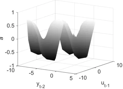
A simple example, similar to that found in Tych et al., 2010, is illustrated in Figure 3 with similar structure and variables to (4) but with the A parameter being a function of two states (5)
8
Figure 3. Illustration of a MSDP. Left hand side, simulated a parameter (offset for clarity). Right hand side, estimated a parameter.
2.0 Arbitrary Sampling within the State Space (OBJECTIVE 1)
For TVP the distance between each parameter value ∆ is based on the temporal distance between each sample and is typically uniform where ∆"=1. For both MSDP and SDP, despite the shift from temporal ordering to arbitrary ordering in the state-space, this is still the case and 𝒑>,= is still estimated with ∆==1. It should be apparent that this is incorrect and ∆= should in fact vary depending on the changing distances between the ordered state values.
This leads to two key changes in the (M)SDP methodology, the first is the calculation of ∆>,= for 𝒑>,= and the second a modification to the random walk models (3) that incorporate a changing ∆. Going back to the equations in (3) focusing on single parameter estimation and defining 𝑎 as 𝒑&,=: if 𝑎s(𝒔
=) is the vth derivative of 𝑎(𝒔=), and the form of the function a(.) is not specified, a data point distant from 𝒔= provides very little information about 𝑎(𝒔=) (Sadeghi, 2006). Using the local polynomial modelling reasoning (e.g. Fan and Gijbels, 1996) only the local data points in the vicinity of 𝒔= are used. Assuming 𝑎(𝒔=) has derivative of order (q+1) at the point 𝒔=, then following Taylor’s expansion for 𝒔 in the local neighbourhood of 𝒔= we have:
𝑎(𝒔) = 𝑎(𝒔=) + 𝑎t(𝒔
=)(𝒔 − 𝒔=) +u
vv(𝒔 w)
7! (𝒔 − 𝒔=)
7+ ⋯ +ux(𝒔w)
G! (𝒔 − 𝒔=)
9
If the value of parameter a and its derivatives with respect to its driving state s are known at the kth
point as 𝒙𝒌= [a(ςk) a’(ςk) a’’(ςk) ⋯ a (q)(ςk)]T and the highest derivative of a(s) with respect to s with sk= ςk : a(q+1)(ςk) = 𝜂
= , where 𝜂=~𝒩|0, 𝜎}7~ and ςk is the approximation point (knot) at sample k, then Taylor’s expansion (6) can be applied in the local neighbourhood of ςk for all derivatives of aresulting in the GRW model with equations:
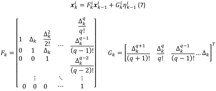
𝒙=> = 𝐹
=>𝒙=(&> + 𝐺=>𝜂=(&> (7)
𝐹= =
⎣ ⎢ ⎢ ⎢ ⎢ ⎢ ⎢ ⎢ ⎡
1 ∆=
∆=7 2!
0 1 ∆=
0 0 1
⋯
∆=G 𝑞! ∆=G(& (𝑞 − 1)!
∆=G(7 (𝑞 − 2)!
⋮ ⋱ ⋮
0 0 0 ⋯ 1 ⎦⎥
⎥ ⎥ ⎥ ⎥ ⎥ ⎥ ⎤
𝐺= = € ∆= GR&
(𝑞 + 1)! ∆=G
𝑞!
∆=G(&
(𝑞 − 1)!… ∆=‚ 3
Where, ∆== ‖ς=− ς=(&‖ is the Euclidean distance between the points ς= and ς=(&.
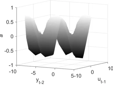
With this generalisation, we now have extended the State Dependent Parameter methodology and to demonstrate the improvement of the addition of arbitrary distance RW algorithm the previous two examples (Figure 1 and 3) are used as comparisons (Figure 4 and 5). We refer to, R2 as the
[image:9.595.123.472.161.309.2]coefficient of determination for a linear regression, or proportion of variance explained by the model.
Figure 4. Comparing equidistant SDP with the arbitrary distance ESDP. Left hand side, equidistant SDP (𝑅7 of 0.9985) from Figure 1. Right hand side, arbitrary distance ESDP (𝑅7 of 1.000). Light grey
10
Figure 5. Comparing A parameter estimates of equidistant MSDP with arbitrary distance ESDP. Left hand side, equidistant MSDP (𝑅7 of 0.9775) from Figure 3 (offset for clarity). Right hand side,
arbitrary distance ESDP (𝑅7 of 0.9810).
Generally, the introduction of arbitrary distance algorithm improves the parameter estimates but with a sizable improvement in the periphery estimates from single states (noticeable from Figure 4) and a reasonable improvement in densely populated estimates from multiple states (reduction of poor estimation in the middle of the saddle shapes from Figure 5).
2.1 Parameter Mapping (OBJECTIVE 2)
Once an ESDP model has been estimated, the surface formed with its driving states can be
interpolated to form a parameter map where using a different data-set of the driving states as the coordinates of the parameters on the map can be used to find a suitably interpolated value of the state-dependent parameter. For SDP this had been done before (Ratto et al., 2007), however it had not been done for MSDP. For example, one of our validation procedures consisted of estimating the MSDP 𝑎…(𝒔&,, 𝒔7) for the training (estimation) subset of temporal samples te=1,..,500 and finding the interpolant to form the parameter map 𝑎†(𝒔&, 𝒔7) followed by using the validation subset samples tv=501,..,1000 to find the interpolated values of 𝑎s(𝒔&,"‡, 𝒔7,"‡) from coordinates 𝒔&,"‡, 𝒔7,"‡.
11
To demonstrate this model validation and data visualisation tool, the model from (5) was used to simulate data for n=2000 where the first half (te=1,..,1000) was used to estimate 𝑎…(𝒔&,"ˆ, 𝒔7,"ˆ) and
then interpolated to find map 𝐴Š(𝒔&, 𝒔7). The second half of the data (tv=1001,..,2000) was then used to interpolate 𝑎s(𝒔&,"‡, 𝒔7,"‡) (Figure 6) and combined with the estimated B parameter from the first
[image:11.595.93.500.184.479.2]half of the data; these two methods of validation can be used to fully validate the ESDP procedure.
Figure 6. Interpolated a parameter for the second half of the data. Left hand side, simulated A (offset for clarity). Right hand side, interpolated a (𝑅7 of 0.9787).
2.2 Model Validation (OBJECTIVE 3)
There are four levels of testing that can be applied to validate the performance of these types of models at the stage of their development. The first two support the DBM model development phase, where the suitability of the model structure becomes apparent, while the third and fourth levels constitutes the final validation steps.
1. Within-sample model fit – 𝑅7 of: model output, estimated A parameter and estimated B parameter (the latter two – for simulated models).
2. One-step ahead prediction model fit 𝑅7 – where the simulation output (y
t) is recalculated
using the estimated parameters instead of the function of states to form the estimated output (𝑦‹") with the regressor values (yt-1, ut-1) still used as above.
3. Full input-output model simulation fit (𝑅"7 )– again where (yt) is calculated but not only using
12
4. Monte Carlo simulations of the full-simulated model using the estimated parameter standard errors with normally distributed parametric variation – generating error bands for the full input-output model simulation to check model sensitivity and uncertainty.
The first of these tests has been done with the 𝑅7 of the estimated parameter for each model supplied within the relevant figure caption and the overall model fit 𝑅7was 0.9943 for (Figure 4) and 0.9959 for (Figure 5). The middle two tests were implemented first for the first half of the data and then secondly for the second half of the data from the previous section; first half, one-step ahead and full model simulation produced 𝑅7 of 0.9973 and 𝑅
"7 of 0.9950 respectively. Second half, one-step ahead and the full model simulation produced 𝑅7 of 0.9908 and 𝑅
[image:12.595.122.474.283.576.2]"7 of 0.9869 respectively. The MC simulations were also implemented on both halves of the data and shows the model stability (Figure 7).
Figure 7. Uncertainty of the full model simulation, validation on the second half of data: 95% percentile band of MC simulations using the estimated parameter standard error with normally distributed parametric variation (zoomed-in for visibility). Rt2 for the first half of the data (training
set) was 0.995.
13
The identification process for estimation period takes into account the prevailing conditions (such as soil saturation), and if they do not change, they are made constant (not an SDP) in the model. These same conditions may be different during the validation period. Enlarging the model would be needed for covering both periods, but this is prohibited by the efficient identification process selecting the parsimonious model for the estimation period.
2.3 Extended State Dependent Parameter (ESDP) Methodology
With updating the variable state-space distancing, addition of multiple dimensional parameter maps and introduction of the latter 2 steps of model validation, the MSDP and SDP methodologies have been updated to perform better (in terms of parameter estimation and model fit) and extended to include more tools for system analysis. This, with the observation that MSDP is a generalisation of SDP to include more than one state, leads to term what is presented here as Extended State Dependent Parameters (ESDP) methodology.
With the inclusion of the following model structure identification procedure, ESDP will have all the tools necessary for analysis of nonlinear dynamic systems in a complete DBM setting.
3.0 Model Structure Identification (MSI) for ESDP (OBJECTIVE 4)
It has to be stated at this point, that the work presented in this section is, by its very nature, a step towards the general structure identification for a very general class of models. Therefore, it should be treated as a pragmatic study, providing constructive directions and effective solutions for a specific class of models, but not the ‘final’ and general answer to the question.
Since the general MSI algorithms for linear TF models are such a useful tool in investigating system dynamics, it is logical to assume MSI for nonlinear SDP models would be just as useful. Historically, SDP has been employed to study specific interactions where the main model structure is pre-selected by the researcher, and the nonlinearity was the main subject of identification.
However, within the realm of nonlinear systems, identification of model structure is not as clearly defined as within the class of LTI (Linear Time-Invariant) models and no well-defined general approach has been developed so far. While model selection within the Nonlinear ARX class (1) is slightly better defined due to the constraints on the TF models, in general model structure identification largely remains an open topic for nonlinear systems.
Most existing approaches to tackling nonlinear structure identification involve assuming some aspect of linearity (Haber and Unbehauen, 1990):
• Breaking a nonlinear system into parallel subsystems with different degrees of nonlinearity (usually static) with at least one dynamic linear subsystem.
• Box models containing static nonlinear and dynamical linear terms such as simple Hammerstein or Wiener models.
• Cascade models with single-valued static (no memory) nonlinear terms, such as the Wiener-Hammerstein cascade model.
• A nonlinear process that can be described by a semi-linear system with signal-dependent parameters where a static polynomial function is assumed for the parameters.
14
The simplifying assumptions for these five types of nonlinear systems lead to easier model
estimation and identification, as the nonlinearities are typically stationary and single-valued (with no memory) whereas for general nonlinear systems these assumptions cannot be made.
For more general nonlinear systems, there are a few structural identification methods:
• Fuzzy Model approach where a linear model is first identified and then fuzzified (Sugeno and Kang, 1988)
• Neural Networks approach, which involves adjusting the weights of layers of ‘neurons’ (that form a network) to identify model structures (Narendra and Parthasarathy, 1990), effectively creating a large number of parametric nonlinear regressions.
• Genetic Algorithms (GA) and Genetic Programming (GP) involves the creation and evolution of model structure from a dataset and; in the former, a set of adaptive algorithms (Whitley, 1994) and in the latter, an existing function library that is chosen by the researcher (Gray, et al., 1998), with Evolutionary Algorithms effectively selecting the ‘fittest’ model structure. This family of techniques could apply to MSDP and will be evaluated in this context in the forthcoming studies.
The issue with Neural Networks and Fuzzy Models is that due to their complexity, even for simple models, they can be unreliable for making model-based predictions because of their high
parameterisation leading to potentially large parametric uncertainty, not to mention the resulting long execution times. By contrast, the aim of this paper is to study a robust and generally usable method with a wide range of applications.
In general, when identifying the structure of a model an important assumption is made prior to choosing the MSI method: is the system linear or nonlinear? If the system is assumed to be linear, then any possible nonlinear aspect of that system will be ignored, and likewise if the system is assumed to be nonlinear, then the dominance of its linear modes may be overlooked, and an overly complex structure may be assumed. The methodology presented here considers both linearity and nonlinearity when identifying the structure of a system. This is particularly important when
investigating state dependencies as the proposed MSI has the flexibility to consider the case of no-state dependency, i.e. a linear system, for a particular dataset. In addition, the methodology presented here considers true nonlinearity, in that the system is nonstationary / time variable. In general, the TF model MSI algorithms find the statistically optimal model structure from the available time-series data by evaluating each possible model through the following process (Young, 2011):
• Estimate the parameters and output of a model candidate.
• Calculate an identification index value that statistically represents the likelihood that this model is the correct one for this data set, or a different model quality index.
• Repeat the above steps for all possible structure combinations.
• The highest or lowest, depending on type of identification index used, is considered the statistical optimum model structure for this data set.
For linear TF models the number of possible models depends on the maximum model polynomial orders (POmax), the number of inputs and the maximum time-delay (δmax) with MSI only needing to
15
For nonlinear ESDP models the number of possible candidate models depends, in addition to the above, on the maximum number of potential states which could drive each of the parameters (S), and on the maximum number of dimensions (Mmax), with MSI required to find the statistically
optimum model polynomial orders and time delay, as well as how many, and which, states drive each parameter.
This additional complexity of model selection creates a non-trivial identification problem, potentially generating numbers of models which would be unrealistic to evaluate in finite time. This is why the polynomial orders are kept pragmatically low as not to introduce headaches and over-complicated models.
3.1 Number of Candidate Model Structures (NCM) to Evaluate
Before an algorithm can be developed for MSI, an understanding of how many models are possible (in the sequel termed number of candidate models (NCM) for more clarity) from a given configuration
of hyper-parameters is required; number of regressors (R), S, Mmax and δmax. Note, to avoid
over-complication the number of n+m parameters from differing polynomial orders is restrained to n=m. In full implementation this need not be the case. This means R gives the number of parameters to estimate (1 parameter per regressor). If polynomial orders were not restrained to n=m, POmax
would also be a hyper-parameter to determine the n+m parameters per model.
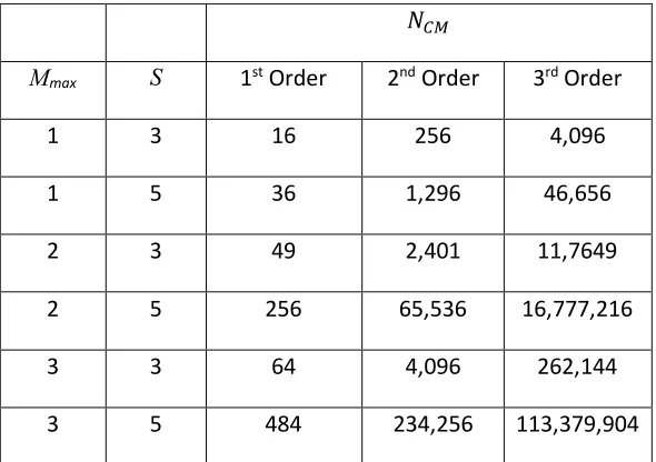
The total number of candidate models for a given set of hyper-parameters is given by (8) and Table 1 illustrates just how quickly the complexity of MSI becomes, as more state variables and higher polynomial orders are considered.
𝑁Œ• = 𝛿0u•× _𝑆 + 1 + ∑ ‘(𝑆 + 1 − 𝑖) ×(“(>) 7 ” ••–—(&
>˜& e
[image:15.595.151.446.549.757.2]™ (8)
Table 1. Showing how the number of candidate models (𝑁Œ•) varies depending on the maximum dimensional space and the number of possible state variables. Polynomial orders are restrained to n=m and δmax=1
𝑁Œ•
Mmax S 1st Order 2nd Order 3rd Order
1 3 16 256 4,096
1 5 36 1,296 46,656
2 3 49 2,401 11,7649
2 5 256 65,536 16,777,216
3 3 64 4,096 262,144
16
However, to create an algorithm to explore each candidate model, other equations are required; their number and form dependent upon R and Mmax:
Number of basic models (𝑁š•) = (𝑀0u•+ 1)™
For the class of models with NARX structure (4), where 𝐴(. ) and 𝐵(. ) are either functions of a number of states (SDP/MSDP) or are constants (coefficients).
𝑦"= 𝑎(. )"(/. 𝑦"(/+ 𝑏(. )"(/. 𝑢"(/ (9)
When Mmax=1 (as in SDP), NBM=4: (numbers in brackets in the lists below are the number of states
influencing that parameter, for example A(0) would mean just a constant parameter, while A(1) would mean A dependent on one state):
1. 𝑦"= 𝑎(0)"(/𝑦"(/ + 𝑏(0)"(/𝑢"(/ 2. 𝑦"= 𝑎(0)"(/𝑦"(/ + 𝑏(1)"(/𝑢"(/ 3. 𝑦"= 𝑎(1)"(/𝑦"(/ + 𝑏(0)"(/𝑢"(/ 4. 𝑦"= 𝑎(1)"(/𝑦"(/ + 𝑏(1)"(/𝑢"(/
When Mmax=2, nBM=9, the 4 from above and the following: 5. 𝑦"= 𝑎(0)"(/𝑦"(/ + 𝑏(2)"(/𝑢"(/
6. 𝑦"= 𝑎(2)"(/𝑦"(/ + 𝑏(0)"(/𝑢"(/ 7. 𝑦"= 𝑎(1)"(/𝑦"(/ + 𝑏(2)"(/𝑢"(/ 8. 𝑦"= 𝑎(2)"(/𝑦"(/ + 𝑏(1)"(/𝑢"(/ 9. 𝑦"= 𝑎(2)"(/𝑦"(/ + 𝑏(2)"(/𝑢"(/
When Mmax=3, nBM=16, the 9 from above and the following: 10. 𝑦"= 𝑎(0)"(/𝑦"(/ + 𝑏(3)"(/𝑢"(/
11. 𝑦"= 𝑎(3)"(/𝑦"(/ + 𝑏(0)"(/𝑢"(/ 12. 𝑦"= 𝑎(1)"(/𝑦"(/ + 𝑏(3)"(/𝑢"(/ 13. 𝑦"= 𝑎(3)"(/𝑦"(/ + 𝑏(1)"(/𝑢"(/ 14. 𝑦"= 𝑎(2)"(/𝑦"(/ + 𝑏(3)"(/𝑢"(/ 15. 𝑦"= 𝑎(3)"(/𝑦"(/ + 𝑏(2)"(/𝑢"(/ 16. 𝑦"= 𝑎(3)"(/𝑦"(/ + 𝑏(3)"(/𝑢"(/
The basic models above may be repeated for different combinations of dependent states, depending on how many are available, for example when Mmax=2 and S=2, basic models number 2,3,7,8 are
repeated twice and the basic model 4 is repeated four times. The formula for the number of possible combinations depends on the basic model (see Appendix A, Table 1 for each formula per basic model).
One aspect that is not taken into consideration here is the possibility of different time-delays for each regressor and each state as that would dramatically increase 𝑁Œ•, which is already
17
One thing that needs to be pointed out is the number of calculations involved in a single model evaluation. For linear MSI the parameters are constant and so only the order of n+m calculations are made. However, for nonlinear MSI the parameters are not fixed and so the order of N×n+m calculations are made. With long series of high frequency data, where the application of nonlinear models would be useful, hundreds of thousands of samples are often used. This requires either long computational times or the utilisation of parallel computation.
However, limiting the model orders, including prior identification of the system’s dominant modes using linear or simply time varying analysis techniques (Young, 1999a) should allow for a pragmatic two-stage procedure. Additionally, the search process is highly ‘parallelizable’, which is not difficult to implement using contemporary multi-processor computers and tools such as Matlab’s Parallel Toolbox.
3.2 Evaluation of each Candidate Model: Noise Variance Ratio (NVR) vs. effective parameterisation level (number of degrees of freedom)
An information value needs to be calculated for each model evaluated in order to determine the optimum model structure; typically, this value is called Information Criterion (IC) and can be formulated in a number of ways (Akaike 1972; Sakamoto, et al., 1986; Young, 2011).
For the MSI methodology presented here the likelihood function (LF) was initially used and compared with Akaike IC (AIC):
𝐴𝐼𝐶 = 2 × 𝑛 u¡− 2 log 𝐿𝐹 (10)
where LF is the likelihood function (calculated as part of the ESDP procedure) and the effective number of parameters (npar), similar in concept to the number of degrees of freedom, is equivalent to a single time varying model coefficient is found from:
𝑑𝑡 = 0.5 × _&¨-© iª™e
-.7©
𝑛 u¡ = i
«"(7 (11)
dt can be interpreted as a subsampling ratio (when dt=2 every second sample is taken with the accompanying loss of temporal resolution – filtering/smoothing) (Ng and Young, 1990), and it reflects the time-scale of variability of the parameter. Naturally, npar is calculated for each of the TVP
(Eq. 10) separately, so the AIC value would be calculated using the total of these values for all the TV parameters.
Normally ESDP optimises the NVR during parameter estimation convergence, however for the proposed MSI methodology the parameters for each candidate model are estimated once with a fixed NVR. This greatly reduces computational time and would render (11) irrelevant as the NVR never changes, thus AIC and LF preformed identically in terms of model identification.
However, through extensive simulation testing using a broad range of both NVR values and nonlinearities within the NARX class of models, it was found that the total number of dependent states had a stronger influence over which model was selected than the effective number of parameters npar, i.e. models with higher numbers of states were being chosen over models with
18
value (12) to offset this bias which was obtained empirically from a review of a broad range of NARX model structures using simulated data to warrant reproducibility.
𝑤 = 0.5 × log&-(1 + 𝑁“) (12)
where, NS is the total number of states used in the candidate model and then the overall IC equation
becomes:
𝐼𝐶 = 𝐿𝐹 + 0.5 × log&-(1 + 𝑁“) (13)
The IC of all evaluated models is sorted and the highest value corresponds to the model structure considered to be statistically optimal.
3.3 Sensitivity of NVR vs. Smoothness of Data vs. Complexity of the Model Sought
Through a search of a broad range of NVR values for several scenarios (such as the simulated examples above, and a complex nonlinear industrial benchmark), it was found that the proposed IC was robust enough to identify the correct model structure for a wide range of NVRs (10-10:10-2).
However, for hydrological data (such as that found in Section 4), it was found that higher NVRs resulted in a different model structure being identified to lower NVRs, e.g. for the example in Section 4, NVRs between 10-10:10-4 identified one model structure and NVRs >10-4 identified a
different model structure.
This is logical as simulated examples are typically simple and built to have one timescale whereas hydrological data is composed from a number of cycles and system dynamics meaning applying different timescales results in different models. Selecting an NVR is similar to selecting a timescale as low NVRs only enable identification of the broader picture and high NVRs provide all the
temporal detail seen in frequently sampled data. 3.4 The Need for Parsimonious Models
As is clearly shown in Table 1, the number of models becomes prohibitively large if too complex models are specified. This is for fixed, pre-selected NVR values. The problem would be compounded if optimising NVR values. This is due to the fact that for each model NVR is optimised (Maximum Likelihood), and the ML objective function response surfaces become very flat for
over-parameterised (mis-specified) model structures, which makes the optimisation much slower. This reinforces the need for parsimonious modelling approach (Young, 2011), not unique to the realm of nonlinear models, but particularly critical in this area.
3.5 Simulated Example
A model of NARX structure similar to (4) was simulated:
𝑦"= 𝑎(𝒔𝟑,𝒕, 𝒔7,")". 𝑦"(&+ 𝑏(1)". 𝑢"(& 𝑡 = 1, . . , 𝑁 (14)
where, 𝑎(𝒔𝟑,𝒕, 𝒔7,")"= 𝑒(𝒔®,¯bc
° (𝒔 °,¯bc °
19
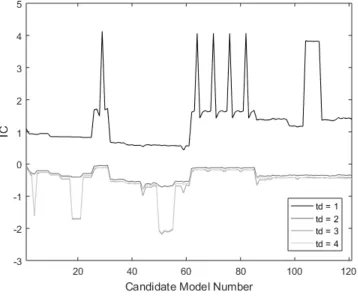
[image:19.595.116.474.133.429.2]sequences with zero mean and unit variance. 484 models were evaluated and formed the IC values (Figure 8) that correctly identified model structure number 35 with a time-delay of 1.
Figure 8. Information Criterion values from the proposed MSI methodology. Highest peak is for model structure number 29 with a time-delay of 1, which corresponds to the model structure in (14). The key observation (Figure 8) is the sensitivity to time-delay, making identifying the time-delay the easiest part of MSI. The four other peaks correspond to candidate models with the same state configuration for a but with b being a single SDP driving by 𝒔&, 𝒔7, 𝒔± and 𝒔² respectively. After identifying the structure, the model was then estimated using ESDP producing a fit a R2 of
20
Figure 9. Illustration of the a parameter. Left hand side, simulated a parameter (offset for clarity). Right hand side, estimated a parameter.
4.0 Streamflow Generation Example (Objective 5)
A commonly used hydrological model in flood simulation is 𝑄 = ℱ(𝑅), where R is rainfall within a catchment, Q is the streamflow per unit basin area (or ‘channel runoff’) and f is a functional representing the dynamic processes involved in translating rainfall into runoff. This model may be described by the equations (1 or 2) in atypical catchment systems where a linear relationship is observed (Ockenden and Chappell, 2011). Rainfall-runoff is however, often a nonlinear process (McIntyre and Al-Qurashi 2009; Beven, 2012), so an SDP methodology may be applied to capture this nonlinearity. Since it is not always clear whether nonlinearity in rainfall-runoff response is caused solely by temporal variations in the moisture state of the whole active hydrological system including rock aquifers, rather than a combination of nonlinear hydrological processes also related to differing rainstorm characteristics (Rodríguez-Iturbe et al., 1982; Chappell et al., 2017), changes in wet-canopy evaporation during storms (Love et al., 2010), diurnal solar radiation effects on soil moisture via transpiration dynamics (Deutscher et al., 2016) or temperature effects on snow melt (Loheide et al., 2009; Mutzner et al., 2015). There is therefore an intrinsic value in applying an ESDP
methodology to discover the dominant mechanism active in the current data set - strictly following the DBM philosophy.
21
where a(.) and b(.) are defined as in (9), with SDP coefficients. The base-line of the flow series is estimated at the same time, in this case as a constant, within the same estimation process. The aim here is to use MSI to identify the most statistically likely state variables, if any, driving parameters a and b and then to apply ESDP to optimise these parameters and finally investigate the parameter-state surfaces for any meaningful physical interpretation of the rainfall-runoff processes.
Even though δ1, δ2 and δ3 could theoretically be different values, for these examples they will all have the same value, determined by MSI and so similar to the commonly used Nash rainfall-runoff model (Nash, 1957). This is done to reduce the number of models MSI needs to evaluate to in order to minimise model complexity and to reduce runtime.
The examples that follow are using 15-minute interval data collected from the 0.76 km2
Nant-y-Craflwyn catchment in upland Wales, UK (Jones and Chappell, 2014; Jones et al., 2014). The available variables are: rainfall, streamflow per unit basin area (‘channel runoff’), air temperature, stream temperature and solar radiation (Figure 10). Rainfall, air temperature and solar radiation were measured at an automatic weather station while stream temperature and streamflow were measured at water quality station and flume, respectively (Fig 1 in Jones and Chappell, 2014). This means the number of candidate models to evaluate is 768 (nCM=256 and assuming one
time-delay with δmax=3). By contrast if each time-delay was to be different then nCM=6912.
[image:21.595.106.482.394.674.2]22
in snow melt or ice melt (Mutzner et al., 2015) or diurnal cycles in transpiration (Deutscher et al., 2016), driven primarily by the diurnal cycle in solar radiation inputs. Within the 15-minute
[image:22.595.139.477.197.491.2]streamflow data for the Nant-y-Craflwyn catchment there is a visible diurnal cycle that corresponds to the solar radiation data (Figure 11). The MSI approach is evaluated to see if solar radiation can be combined with rainfall data to derive a more complete DBM model of the drivers of streamflow response at this location.
Figure 11. Showing the diurnal-modulated nature of the streamflow records for the Nant-y-Craflwyn stream as compared to that found in the solar radiation (both have been standardised for easy of
comparison). This is picked-up by the state dependency estimate of the a parameter. Hourly sampling rate has been chosen for this model to avoid oversampling. The 15-minute data was converted into hourly data, where the rainfall was totalled over the hour and the other variables were pre-processed using an Integrated Random Walk (IRW) smoothing and decimation algorithm from the Captain Toolbox to limit their spectrum to avoid bias (Young et al., 2007).
MSI identified a structure with the decay coefficient dependent on solar radiation and rainfall with time-delays of 1 hour. ESDP produced an optimised model with an R2 of 0.998, estimated A
parameter with range 0.95-1.06 (dimensionless) and constant b (referred to as ‘effective rainfall coefficient’ in Young 2003) of 2.3x10⁻³ with units consistent with observations of discharge.
23
allows a useful representation of the surface (Figure 12) and its subsequent parameterisation for simulation purposes, conveniently including a measure of uncertainty of the smoothed surface.
Figure 12. Decay coefficient and its two dependent states. Left: 3D visualisation of the decay coefficient and the states. Right: projection plots of each state/decay coefficient vs the other
state/decay coefficient.
24
Figure 13. Comparing the decay coefficient estimates to its driving states. Top, comparing the standardised values of the decay coefficient and radiation. Bottom, comparing the standardised
values of the decay coefficient and rainfall.
It is worth noting that this interpretation of the a coefficient is not the same as for Linear Time Invariant systems (LTI) where the value larger than one means the system is unstable, and the values lower than one relate to the recession process of the autonomous (no input) solution. This does not hold for nonlinear (time varying) systems, which are analysed here. Such values of similar SDP parameters have been seen in previous publications (Young, 2000; Young, 2003), while Ratto et al (2007) have limited the a coefficient to not go above one, based on their specific application. In this case leaving a to track unconstrained is a part of the DBM identification process; any physical constraints can be included at the final application stage.
As noted earlier, the apparent diurnal cycle in streamflow may be caused by diurnal cycles in transpiration losses from the subsurface pathways generating streamflow (Graham et al., 2013; Deutscher et al., 2016) or diurnal cycles in air temperature affecting the production of snowmelt (Loheide et al., 2009), but may also be caused by residual thermal artefacts in the pressure transmitter output (Liu and Higgins, 2015; Moore et al., 2016). For the diurnal cycles in the Nant-y-Craflwyn time-series, in-situ field tests show that all of the cyclical behaviour may be explained by residual thermal artefacts. The modelling approach would, however, have been able to quantify the diurnal component of response if it had been caused by transpiration or snowmelt effects, as seen within other catchments.
4.1 Validation
The validation processes described in section 2.2 were applied to the above hydrological data and showed good model validity (Figure 14) with the one-step ahead and full model simulation having R2
25
Figure 14. One-step ahead and full model simulation with uncertainty: 95% percentile band of MC simulations using the estimated parameter standard error with normally distributed parametric
variation. 5.0 Conclusions
The paper unified and improved upon the SDP and MSDP methodologies to form a Generalised State Dependent Parameter methodology. In addition, this paper introduced a generalised Model
Structure Identification methodology that allows for a closer following of the DBM approach to investigating nonlinear system dynamics. The introduction of the arbitrary RW not only generalised the methodology but also improved the parameter estimates.
The MSI approach to identification of this class of nonlinear systems allows researchers to
statistically explore interactions between system variables for a specific process and to give insights into which variables are more important to that process. It also enhances the DBM nature of ESDP by more rigorously determining the model structure, not relying on the researcher’s preconceptions. The ‘brute force’ nature of the algorithm could lead to computational runtime limitations if dealing with many variables and very long data sets, but this is a minor limitation given the ever-increasing power of computers and the option of parallel computation.
The parameter map allows the outputs of ESDP to be quickly utilised for scenario analysis and on-line simulation of live events.
26 5.1 Further Developments
Two groups of developments aimed at improving the usability and applicability of the MSI/MSDP methods may be identified at this stage.
1. Generalisation of the MSI methodology:
• Removal of the constraint of n=m on polynomial orders – greatly increasing the number of models to evaluate but allowing closer following of the DBM approach.
• To other models (multiple inputs, ARMA structures etc.), with the possibility of leading to the future development of an algorithm that chooses the model type as well as the structure.
2. Numerical effort is a serious consideration in this case. Applicability of the method, which naturally involves a structure search and optimisation based estimation, is limited in the current implementation by the time taken by the algorithm, mainly the structural identification search. Thus:
• Only single-input-single-output models were demonstrated but the extension into multiple input and even multiple output is possible – it would drastically increase the number of models to evaluate as seen from Table 1.
• Currently time-delays are fixed, in that all time-delays have the same value.
Allowing MSI to evaluated models with several different time-delays would enhance the exploration of nonlinear dynamics – it would dramatically increase the number of models to evaluate.
• For some systems time-delay can be state dependent and so introducing state dependent time-delay would benefit the modelling of those systems – it would also heavily increase the number of models to evaluate.
5.2 Software Availability
Matlab ESDP library is available from the corresponding author upon request, after further testing it will be incorporated in the CAPTAIN Toolbox. It is recommended to use the current version of the CAPTAIN toolbox for initial transfer function and basic, single state dependency SDP analysis. CAPTAIN Toolbox is available from Lancaster University at the link below:
http://www.lancaster.ac.uk/staff/taylorcj/tdc/download.php
6.0 References
Akaike, H. 1972. Information theory and an extension of the maximum likelihood principle. Proc. 2nd Int. Symp. Information Theory, Supp. to Problems of Control and Information Theory, 267-281. Ampadu, B., Chappell, N. A., Tych, W. 2015. Data Based Mechanistic modelling optimal utilisation of raingauge data for rainfall-riverflow modelling of sparsely gauged tropical basin in Ghana.
Mathematical Theory and Modelling, 5(8), 29-49.
27
Beven, K. J., 2012. Rainfall-Runoff Modelling: The Primer. 2nd Ed. Wiley-Blackwell.
Chappell, N.A., Jones, T.D., Tych, W., Krishnaswamy, J. 2017. Role of rainstorm intensity
underestimated by flood models: emerging global evidence from subsurface-dominated watersheds.
Environmental Modelling and Software, 88, 1-9.
Deutscher, J., Kupec, P., Dundek, P., Holík, L., Machala, M., Urban, J. 2016. Diurnal dynamics of streamflow in an upland forested micro-watershed during short precipitation-free periods is altered by tree sap flow. Hydrol. Process. 30, 2042
Gou, L. 1990. Estimating time-varying parameters by the Kalman filter based algorithm: stability and convergences. IEEE Transactions on Automatic Control, 35(2), 141-147.
Graham, C. B., Barnard, H.R., Kavanagh, K.L., Mc Namara, J.P. 2013. Catchment scale controls the temporal connection of transpiration and diel fluctuations in streamflow. Hydrol. Process. 27, 2541– 2556.
Gray, G. J., Murray-Smith, D. J., Li, Y., Sharman, K, C., Weinbrenner, T. 1998. Nonlinear model structure identification using genetic programming. Control Engineering Practice, 6, 1341-1352. Fan, J., Gijbels, I. 1996. Local polynomial modelling and its applications: monographs on statistics and applied probability66, (Vol. 66). CRC Press.
Gu, C. 2013. Smoothing Spline ANOVA Models. New York: Springer-Verlag New York Inc.
Haber, R., Unbehauen, H. 1990. Structure Identification of Nonlinear Dynamic Systems – A Survey of Input/Output Approaches. Automatica, 26(4), 651-677.
Jones, T., Chappell, N. A. 2014. Streamflow and hydrogen ion interrelationships identified using data-based mechanistic modelling of high frequency observations through contiguous storms. Hydrology Research, 45(6), 868-892
Jones, T.D., Chappell, N. A., Tych, W. 2014. First dynamic model of dissolved organic carbon derived directly from high frequency observations through contiguous storms. Environmental Science and Technology, 48(22), 13289-13297.
Kalman, R.E. 1960. A new approach to linear filtering and prediction problems, Journal of Basic Engineering, 82(1), 35–45.
Li, Y., Ryu, D., Western, A. W., Wang, G. J. 2013. Assimilation of stream discharge for flood
forecasting: The benefits of accounting for routing time lags. Water Resources Research, 49(4), 1887-1990.
Liu, Z., Higgins, C.W. 2015. Does temperature affect the accuracy of vented pressure transducer in fine-scale water level measurement? Geosci. Instrum. Methods Data Syst. 4, 65–73.
28
Love, D., Uhlenbrook, D., Corzo-Perez, G., Twomlow, S., van der Zaag, P. 2010. Rainfall–interception– evaporation–runoff relationships in a semi-arid catchment, northern Limpopo basin, Zimbabwe,
Hydrological Sciences Journal, 55(5), 687-703
McIntyre, N., Al-Qurashi, A. 2009. Performance of ten rainfall-runoff models applied to an arid catchment in Oman. Environmental Modelling & Software, 24(6), 726-738.
McIntyre, N., Young. P. C., Orellana, B., Marshall. M., Reynolds, B., Wheater, H. 2011. Identification of nonlinearity in rainfall-flow response using data-based mechanistic modelling. Water Resources Research, 47(3), doi:10.1029/2010WR009851.
Moore, M.F., Vasconcelos, J.G., Zech, W.C., Soares, E.P. 2016. A procedure for resolving thermal artifacts in pressure transducers. Flow Meas. Instrum. 52, 219-226.
Mutzner, R., Weijs, S. V., Tarolli, P., Calaf, M., Oldroyd, H. J. 2015. Controls on the diurnal streamflow cycles in two subbasins of an alpine headwater catchment. Water Resources Research, 51(5), 3403-3418.
Narendra, K, S., Parthasarathy, K. 1990. Identification and Control of Dynamical Systems Using Neural Networks. IEEE Transactions on Neural Networks, 1(1), 4-27.
Nash, J.E. 1957. The form of the instantaneous unit hydrograph. Int. Assoc. Hydrol. Sci., General Assembly of Toronto., Publ, 45, 114–119.
Ng, C. N., Young, P. C. 1990. Recursive estimation and forecasting of non-stationary time series.
Journal of Forecasting, 9(2), 173-204.
Ockenden, M. C., Chappell, N. A. 2011. Identification of the dominant runoff pathways from data-based mechanistic modelling of nested catchments in temperate UK. Journal of Hydrology, 402(1-2), 71-79.
Ratto, M., Young, P.C., Romanowicz, R., Pappenberger, F., Saltelli, A., Pagano, A. 2007. Uncertainty, sensitivity analysis and the role of data based mechanistic modeling in hydrology, Hydrol. Earth Syst. Sci, 11, 1249-1266.
Rodríguez-Iturbe, I., Gonzales-Sanabria, M. and Camano, G. 1982. On the climatic dependence of the IUH: a rainfall-runoff theory of the Nash model and the geomorphoclimatic theory. Water Resour. Res., 18, 887-903.
Sadeghi, J. 2006. Modelling and control of non-linear systems using state-dependent parameter (sdp) models and proportional -integral-plus (PIP) control method. Ph.D Thesis, Lancaster University, December.
Sakamoto, Y., Ishiguro, M., Kitagawa, G. 1986. Akaike information criterion statistics. Tokyo: KTK Scientific Publishers.
29
Sugeno, M., Kang, G. T. 1988. Structure Identification of Fuzzy Model. Fuzzy Sets and Systems, 28, 15-33.
Taylor, C.J., Chotai, A., Young, P. C. 2009. Non-linear control by input-output state variable feedback pole assignment. International Jounral of Control, 82(6) 1029-1044.
Tych, K., Wood, C., Tych, W. 2014. A simple transfer-function-based approach for estimating material parameters from terahertz time-domain data. IEEE Photonics Journal, 6(1).
Tych, W., Sadeghi, J., Smith, P. J., Chotai, A., Taylor, C. J. 2012. Multi-state Dependent Parameter Model Identification and Estimation. In: Wang, L., Garnier, H. ed. System Identification,
Environmental Modelling, and Control System Design. Springer London, 191-210. Whitley, D. 1994. A genetic algorithm tutorial. Statistics and Computing, 4(2), 65-85.
Young, P. C. 1999a. Data-based mechanistic modelling, generalised sensitivity and dominant model analysis. Computer Physics Communications, 117, 113-129.
Young, P. C. 1999b. Nonstationary time series analysis and forecasting. Progress in Environmental Science, 1, 3-48.
Young, P. C. 2000. Stochastic, dynamic modelling and signal processing: time variable and state dependent parameter estimation. Nonlinear and nonstationary signal processing, 74-114.
Young, P.C., McKenna, P., and Bruun, J. 2001. Identification of nonlinear stochastic systems by state dependent parameter estimation, Int. J. Control, 74, (18), 1837–1857.
Young, P. C. 2003. Top-down and data-based mechanistic modelling of rainfall-flow dynamics at catchment scale. Hydrol. Process. 17, 2195-2217.
Young, P. C., Garnier, H. 2006. Identification and estimation of continuous-time, data-based mechanistic (DBM) models for environmental systems. Environmental modelling & software, 21(8), 1055-1072.
Young, P. C., Castelletti, A., Pianosi. F. 2007a. The data-based mechanistic approach in hydrological modelling. In: Castelletti, A and Sessa R. S. eds. Topics on System Analysis and Integrated Water Resource Management. Amsterdam: Elsevier. 27-48.
Young, P.C., Taylor, C.J., Tych, W., Pedregal, D.J. 2007b. The Captain Toolbox. Centre for Research on Environmental Systems and Statistics, Lancaster University, UK. Internet:
www.es.lancs.ac.uk/cres/captain
30 Appendix A – Additional MSI Information
Table 1. Formula for the number of model combinations when R=2, Mmax=2. S is the number of possible driving states.
Basic Model (from 3.1)
Formula for number of combinations
Examples S=2 S=3
1 = 1 1 1
2 = 𝑆 2 3
3 = 𝑆 2 3
4 = 𝑆™ 4 9
5 = 0.5𝑆7− 0.5𝑆 1 3
6 = 0.5𝑆7− 0.5𝑆 1 3
7 = 0.5𝑆±− 0.5𝑆7 2 9
8 = 0.5𝑆±− 0.5𝑆7 2 9
9 = 0.25𝑆²− 0.5𝑆±+ 0.25𝑆7 1 9