Flow Injection Analysis of industrial water samples

(1)

Flow Injection Analysis of industrial water

samples

by

Agata Dominika Makas, BSc (Hons)

A dissertation submitted to the Lancaster University for the

degree of Master of Science (by research) in Chemistry

(2)

Abstract

An automated version of Flow Injection Analysis (FIA) instrumentation has been designed and evaluated for the quantitative determination of chemical oxygen demand (COD) for industrial samples. The distinct advantages over conventional COD assays are the significantly reduced analysis time (FIA complete in 10 min, compared with conventional COD assay times of 120 min); simplified sample handling; significantly reduced sample volume (less than 1 cm3_{for FIA); significantly reduced reagent consumption; and the avoidance of} highly toxic reagents (such as CrVI+_{). The FIA system developed for this project} included automation with a microcontroller, which enabled automatic sample introduction, which removed imprecision associated with the equivalent manual process.

(3)

Declaration

No portion of the work referred to this dissertation has been submitted in support of an application for another degree qualification for this or any other university or institute of learning.

(4)

Acknowledgements

At the beginning of the project I would like to thank Professor Peter Fielden who has supervised me through this study. He also inspired me to choose this particular subject.

In addition, I would like to thank Dr Sara Baldock who helped me with my project and Crown Paints Ltd. Company (Darwen, Lancashire) for access to their water samples.

(5)

List of figures

Figure 1: Batch process. R indicates analytical reagent(s), S is the sample,

RS is the reaction product, T is time[4]_{. ... 12}

Figure 2: Sample dispersion and signal profiles in the tubing during FIA[5]_{. ... 12}

Figure 3: Laminar flow with parabolic shape (A) and bullet shaped, three-dimensional concentration gradient[5]_{. ... 13}

Figure 4: Difference in laminar and turbulent flow in the tubing[6]_{. ... 13}

Figure 5: Simple flow injection manifold used in FIA[11]_{. ... 14}

Figure 6: Depiction of the working principles of a spectrophotometer[16]_{. ... 16}

Figure 7: Detector response depends on the wavelength of the incident photons[17]_{. ... 17}

Figure 8: Two variations for the conventional Industrial Method for COD determination[29]_{. (i) represents the method that requires titration using} hazardous reagents (details presented in Figure 9) and expensive chemicals and (ii) shows the safer method used by Crown Paints Ltd. ... 19

Figure 9: Procedure of the potassium dichromate method for COD, used in industry[23]_{. ... 20}

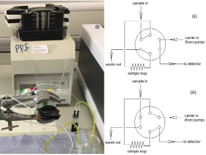
Figure 10: (i) Picture of the primary FIA system used for preliminary analysis. (ii) Presents the position of the valve while filling the loop and (iii) shows the position when running the sample. ... 22

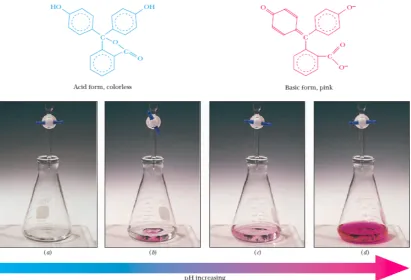
Figure 11: Show the acid and base forms of phenolphthalein, an indicator commonly used in the titration of strong acid with strong base. (a) The acidic solution is initially clear. (b) Adding base makes solution pink but the colour disappearing after swirling. (c) The first permanent pink indicates the endpoint of titration. (d) If the solvent becomes vividly coloured, it means base is in excess[30]_{. ... 23}

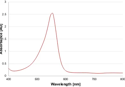
Figure 12: Spectrum of maximum absorbance at 550 nm for the acid and base analysis with phenolphthalein as the indicator. ... 24

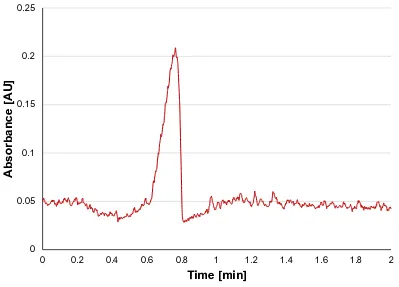
Figure 13: Spectrogram presenting acid/base titration at 550 nm. ... 25

(8)

(9)

(10)

List of tables

(11)

1 Introduction

The aim of the following study is to determine the potential of flow injection analysis (FIA) as an alternative technique for chemical oxygen demand (COD) measurements commonly used in industry.

The objectives of this study are to:

- review and adapt the COD method from the literature by Korenaga & Ikatsu (from 1981)[1]_,

- select the best operating conditions (i.e. temperature, time and reagents),  - to experimentally obtain and analyse of UV-vis spectrograms associated with the COD measurement process,

- investigate and solve problems that occurred during the performance of the experiment,

- develop a calibration procedure with construction and usage of calibration graphs over a useful range of sample concentrations and

- analyse of samples supplied by Crown Paints and compare of the results of the FIA procedure against those obtained from the supplier’s COD analyser.

Flow Injection Analysis (FIA)

(12)

Figure 1: Batch process. R indicates analytical reagent(s), S is the sample, RS is the reaction product, T is time[4]_.

The physical foundations of FIA are related to dispersion and diffusion. Treatment of solute dispersion in a tube considers the relation between axial and radial dispersion on the shape of a sample plug as it moves downstream at a constant flow rate under laminar flow conditions as shown in Figure 2 and Figure 3.

[image:12.595.171.468.442.677.2]

(13)

Figure 3: Laminar flow with parabolic shape (A) and bullet shaped, three-dimensional concentration gradient[5]_.

The flow velocity (𝑢) may be calculated using equation:

𝑢 = 2𝑢 % &1 − )*₊,-. /00₁ 2 where 𝑢 % is mean flow velocity /33₄ 2, r is radial distance [mm], a is radius of the channel [mm].

Diffusion is the spreading of molecules or atoms due to a gradient in concentration. Diffusion length (L, distance travelled by reagents) in the tubing can be calculated using the following equation, which is based on Fick’s Law. 𝐿-_{= 2𝐷𝑡 [𝑚𝑚}-_] _where_D_{is diffusion coefficient (in aqueous solution it has} a value between 6 ∙ 10>?_{to 2 ∙ 10}>? 0@

1 ), t is time [s].

Movement of solvent may be descried by calculating the Reynolds Number. Mixing will change in different kind of flows.

The Reynolds number is the ratio of inertial forces to viscous forces and is a convenient parameter for predicting if a flow condition will be laminar or turbulent (Figure 4).

Re < 2000, particles move in straight lines, rare in water systems

Re > 4000, irregular movements of particle in the fluid, most common in water systems

(14)

𝑅𝑒 =

CDE

F

G

H IIJ ∙

II K ∙00 H K ∙II

= 1L

where Re is Reynolds number, u is flow

velocity /33

4 2, p is density of the fluid

/

M

33J

2

,

𝑣

is kinematic viscosity of the

fluid / M

4 ∙332 and L is characteristic linear dimension [mm].

FIA is simple, quick, versatile and gives quantitative results[7]_{. Analysis does not} require large volumes and complex sample preparation. In every technique, the possibility of reconstruction and reproduction is the most important part. Flow injection analysis gives certainty that the sample volume does not significantly change between injections. Therefore, automation makes FIA a perfect technique for analysis. What is more automation helps in cost and hazard reduction, and the implementation of control and timing[8]_{. Furthermore,} automation reduces the risk of contamination[9]_{. Since FIA is an automated} technique, it significantly reduces human mistakes which leads to increased precision and improved reproducibility[4], [10]_.

Figure 5: Simple flow injection manifold used in FIA[11]_.

(15)

Components used to build the FIA system are relatively inexpensive. Moreover, the system can be easily modified to achieve optimised results or adapted to meet any type of task without complex changes[12]_{. Thus, the FIA technique} is widely used in many areas. For example: chemical analysis, pharmaceutical, environmental and clinical chemistry, online monitoring of biotechnology, food and agriculture analysis[2], [7], [10]_{. Nowadays, monitoring waste and its treatment} has become a big challenge, but even FIA may be used in that area[8]_.

Versatility of FIA coupled with various detectors

Various detectors may be coupled with a flow injection analysis system. The perfect detector should have a low noise level, a fast and linear response over a wide concentration range and high sensitivity[12]_.

Mostly used are detectors that measure: fluorescence, atomic absorption, pH or flame emission. What is more FIA system may be coupled with ion selective electrodes, a potentiostat or even high performance liquid chromatography (HPLC)[8], [12], [13]_.

A spectrophotometer coupled with a FIA system gives a setup which provides fast analysis with good precision. Moreover, it is easy to operate and relatively cheap[9]_{. Most of the analyses are done on – line which means the sample} is analysed immediately once it reaches the detector in the flow cell. Another method is to collect a sample and put it in the container to be analysed as a ‘static’ sample[14]_.

(16)

Detector used during the experiment – Spectrophotometer

An Agilent Technologies Cary 60 UV-Vis Spectrophotometer was used as a detector throughout the project. A xenon pulse lamp is the source of light and it provides both visible and UV light. The light beam (dimensions 1.5 x 1.0 mm) strikes the holographic diffraction grating (dimensions 27.5 x 35 mm with 1200 lines/mm), which separates the light into its component wavelengths (190 – 1100 nm). The grating is rotated so that only a specific wavelength of light reaches the exit slit. Then the light interacts with the sample. Then the detector measures the transmittance and absorbance of the sample. Detectors in the instrument used are dual silicon diodes (photodiode). A silicon diode detector enables the widest range of wavelengths to be measured without any loss of the sensitivity (Figure 7). Light transmitted through a material reduced exponentially as it travels through the sample. Beer-Lambert Law is the linear relationship between absorbance and concentration of an absorbing species. Absorbance is dimensionless and is described by the following equation:

𝐴 = 𝜀𝐿𝐶 /𝑀 ∙ 𝑐𝑚 ∙

T

U ∙ V0

= 12

where

𝜀

is wavelength dependent

[image:16.595.108.526.468.703.2]

coefficient /_{W ∙ X3}T 2, L is a path length [cm] and C is concentration [M].

(17)

Figure 7: Detector response depends on the wavelength of the incident photons[17]_.

FIA vs Conventional Industrial Method for COD analysis

The most popular industrial method for COD analysis is based on the method that employs dichromate chemistry for the oxidation[18]_{. That includes usage} of hazardous, toxic and expensive chemicals such as potassium dichromate (K2Cr2O7), mercury sulfate (HgSO4), silver sulfate (Ag2SO4) or ferroin indicator [Fe(o-phen)3]SO4. A silver compound is added as a catalyst to promote the oxidation of certain classes of organic compounds. A mercuric compound may be added to reduce the interference from oxidation of chloride ions. After the oxidation is completed, the amount of dichromate consumed is determined titrimetrically, titration is done using ferrous ammonium sulphate[19]_{. Either,} the amount of reduced chromium or the amount of unreacted dichromate can be measured.

The process takes more than 2 hours (as a manual analysis)[20]–[22]_{. All steps} required to be done before the analysis are shown in Figure 9. In the comparison of FIA and the Industrial Method for COD measurements is presented.

(18)

All organic matter in the sample gets oxidized by a known excess of potassium dichromate in presence of sulfuric acid. Temperature in COD digester allows reaction to happen, then remaining, unreduced dichromate is determined by titration against ferrous ammonium sulphate, using ferroin as an indicator. The dichromate consumed by the samples is equivalent to the amount of oxygen required to oxidize organic pollutions in the water sample[23], [24]_.

Table 1: Comparison of FIA and Industrial Method for COD analysis.

Flow Injection Analysis Industrial Method (potassium dichromate)[23], [25]

Time of

analysis Less than 10 min About 3 hours

Chemicals Fairly safe at concentrations

and quantities used

Significantly hazardous reagents and waste (including mercury)

Analysis Automated Requires titration and adding chemicals using pipettes

Typical sample volume

20µl 2.5 ml

Detection range

5 - 198 mg/l (range used

during this experiment) 3 - 900 mg/l

Equipment Mostly available in every

laboratory

Mostly available in every laboratory but also need COD

digester

Sample preparation

None or just dilution with distilled water to match

concentration range

Complex, including adding K2Cr2O7 and H2SO4 as well as

digestion

Calculation of COD concentration

Equation obtained from calibration graph eg. 𝐶𝑂𝐷 =Z[1 >\.?^_`

>TT?._a

More complicated equation

𝐶𝑂𝐷 =[(𝐴 − 𝐵) ∗ 𝑁 ∗ 8 ∗ 1000] 𝑉

A – volume of ferrous ammonium sulfate for blank

B – volume of ferrous ammonium sulfate for sample

(19)

From comparison of the two COD methods it is possible to see that FIA has many more advantages compared with the conventional Industrial Method. Flow injection analysis is much faster (including analysis and sample preparation) and safer for an operator (does not require use of any hazardous chemical); it does not even require an operator. It needs much smaller sample volumes, while the detection limit is still comparable. Furthermore, in the FIA calculation of the COD concentration of the sample it requires only the absorbance value of the peak height while an industrial method requires more complex calculations and more data to be known.

Nowadays, more laboratories start to use safer and faster techniques which excludes titrations using hazardous and toxic chemicals (Figure 8 ii), Crown Paints Ltd. is one of them. However, this technique still takes more than 2 hours and mercury – containing reagents are used. The method requires sample preparation and specially ordered COD Reagent vials (according to VWR website the cost of the vials vary from £1.50 to £1.90 each[26]_).

One should know that COD vials are delivered from the USA, that will make costs higher. What is more, one must have an idea what the COD concentration may be before the analysis, because vials have various ranges (from 0 – 150 mg/l and 0 – 15 000 mg/l)[27], [28]_.

Figure 8: Two variations for the conventional Industrial Method for COD determination[29]_{. (i) represents the method that requires titration using} hazardous reagents (details presented in Figure 9) and expensive chemicals

(i)

[image:19.595.108.527.384.698.2]

(20)

[image:20.595.126.509.126.647.2]

(21)

2 Project Part I

(22)

Flow Injection Analysis system used for preliminary analysis

[image:22.595.110.527.283.597.2]

The project was started by setting up a Flow Injection Analysis system and running a simple experiment in order to understand the principles of the technique. Figure 10 shows the picture of how the FIA system was set up. It was made up from a two-way, six-port rotary valve, a set of tubing, a peristaltic pump, a flow cell QS 0.300 and an UV-Vis spectrophotometer. The pump used throughout the experiment was a Gilson® Minipuls 3 and an Agilent Technologies Cary 60 UV-Vis Spectrophotometer was used as the detector.

(23)

Investigation of FIA system using an acid/base reaction

The acid/base reaction between hydrochloric acid (HCl) and sodium hydroxide (NaOH) in the presence of phenolphthalein was introduced to run samples through the FIA system using a reaction that resulted in a noticeable colour change as shown in Figure 11. The experiment began with preparing 1 litre of 0.1 M of each analyte from stock solutions. Available reagents had to be diluted to obtain the required concentrations. Dilution was done as follows: 50 ml of 2 M NaOH to get a 1 litre of 0.1 M and 100 ml of 1 M HCl to get a 1 litre of 0.1 M, pH indicator was already available at the university and used as given. Phenolphthalein was prepared using 50% ethanol to give 0.1% m/V solvent.

[image:23.595.113.525.326.606.2]

(24)

Indicators change colours in different environments. Phenolphthalein becomes pink in basic environment. Colour changing occurs where there is the same amount of both forms present in the mixture, the equilibrium lies exactly in the middle:

𝐻𝐼𝑛 ⇌ 𝐻

m

+ 𝐼𝑛

>

𝑝𝐾𝑎 =

/𝐻

+₂_r_𝐼𝑛−_s

r𝐻𝐼𝑛s

when equilibrium is in the centre then:

[𝐼𝑛

>

] = [𝐻𝐼𝑛]

so

𝑝𝐾𝑎 = 𝐻

m _{which is}

_{𝑝𝐾𝑎 = 𝑝𝐻}

pKa = 9.7 [30]

Based on that information, one knows that the indicator will change colour when the pH is the same value as its pKa value.

[image:24.595.115.518.448.727.2]

Firstly, the wavelength of the maximum absorbance had to be specified. To do so, 5 ml of HCl with 0.5 ml of phenolphthalein and 5 ml of NaOH were mixed and transferred into a cuvette. The spectrum was recorded between 400 - 800 nm and the highest absorbance was at 550 nm (Figure 12). Thus, it was the chosen wavelength to run all samples with hydrochloric acid, sodium hydroxide and phenolphthalein.

Figure 12: Spectrum of maximum absorbance at 550 nm for the acid and base analysis with phenolphthalein as the indicator.

0 0.5 1 1.5 2 2.5 3

400 500 600 700 800

Absorbance [AU]

(25)

[image:25.595.121.520.96.383.2]

Figure 13: Spectrogram presenting acid/base titration at 550 nm.

A carrier solution of 100 ml of HCl and 1 ml of pH indicator were mixed and delivered from the flask by the peristaltic pump. The sample, NaOH in this case, was supplied by the syringe to fully fill the loop (74.6 µl). The carrier solution was colourless because phenolphthalein gives a pink colour only in basic solution (Figure 11). The valve position was changed (sample injected), and then the reaction began. It was possible to see a colour change which was measured by the spectrophotometer (Figure 13).

0 0.05 0.1 0.15 0.2 0.25

0 0.2 0.4 0.6 0.8 1 1.2 1.4 1.6 1.8 2

Absorbance [AU]

(26)

Pump calibration and optimisation of the pump speed

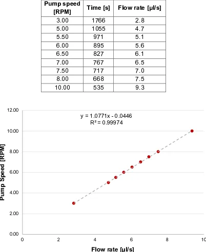
The peristaltic pump was calibrated by measuring the time needed to fill a 5 ml-measuring cylinder. The flow rate (F) was calculated using the following equation:

𝐹 =

u

v

/

wx

[image:26.595.115.517.232.724.2]

1

2

where V is volume and equals 5 ml = 5000 μl and t is time [s].

Table 2: Table showing data from the pump calibration used in the calibration graph from Figure 14.

Pump speed

[RPM] Time [s] Flow rate [μl/s]

3.00 1766 2.8

5.00 1055 4.7

5.50 971 5.1

6.00 895 5.6

6.50 827 6.1

7.00 767 6.5

7.50 717 7.0

8.00 668 7.5

10.00 535 9.3

Figure 14: Pump calibration graph based on data from Table 2.

y = 1.0771x - 0.0446 R² = 0.99974

0.00 2.00 4.00 6.00 8.00 10.00 12.00

0 2 4 6 8 10

Pump Speed [RPM]

(27)

The main conclusion from calibration graph analysis is that the flow rate is predictable and linear over the range tested. In that analysis, it can be calculated based on the equation from it (y = 1.0771x - 0.0446). However, it may differ when using a different kind and length of tubing. Thus, new calibrations must be done when components of the pump system are changed.

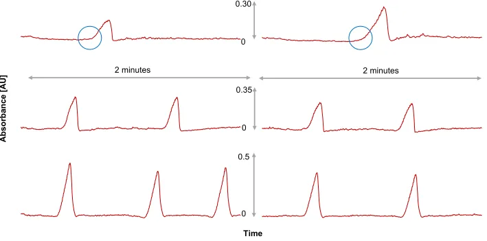
The optimised pump speed has been selected based on the peak shape (Table 3). In Figure 15 the number of peaks in each analysis corresponds to the number of sample injections. In the two slowest analyses, only one sample has been analysed, in those that are faster two or three samples have been injected. One can see that the best peaks are in analyses (v) and (vi). Peaks are high, narrow and there is no fronting as in the first four analyses (sample peak with fronting has been highlighted by a blue circle in the first two spectrograms). Based on the optimisation results the best pump speed has been set as 11.0.

Table 3: Summary of spectrograms analysis from Figure 15.

Analysis Pump speed [RPM] Description

i 5.0 Small and broad peaks, fronting

present

ii 7.0

iii 9.0 Peaks still small and some fronting present

iv 10.0

v 11.0

High and narrow peaks

(28)

[image:28.842.57.766.126.477.2]

Figure 15: Spectrograms used to select the best pump speed. (i) indicates speed 5.0, (ii) speed 7.0, (iii) speed 9.0, (iv) speed 10.0, (v) speed 11.0 and (vi) speed 11.5. Additionally (i) and (ii) present fronting of peaks marked by a blue circle. Each analysis last 2 min.

2 minutes 2 minutes

Ab

s

o

rb

an

c

e

[A

U

]

0.30

0

Time

0.5

0 0.35

(29)

2.4 Preliminary optimisation using food dye samples

To understand the principles of flow injection analysis, the first experiment was done only with distilled water and blue food dye (blue food colouring by Sainsbury’s). A splash of dye (unknown volume) was diluted in the distilled water and used as a sample.

The first step of primary analysis required the appropriate wavelength to be established. The graph below shows maximum absorbance for the analysed sample at 620 nm. For analysis, a cuvette with 10 mm path length and 4.5 ml volume was used.

Figure 16: Spectrum of blue dye solvent shows maximum absorbance (at 620 nm) of sample used in primary analysis.

Based on primary analysis, the wavelength, which was used in the analysis of the food dye was 620 nm (Figure 16). In Figure 17, which presents analysis of blue dye samples, three peaks correspond to three sample injections are shown. The third peak is smaller than the other two probably due to insufficient loop filling.

0 0.2 0.4 0.6 0.8 1

400 450 500 550 600 650 700 750 800

Absorbance

[AU]

[image:29.595.112.511.306.588.2]

(30)

[image:30.595.115.513.98.382.2]

Figure 17: Spectrogram of flow injection analysis of blue food dye.

The loop length (H) was 95 mm with diameter (r) of 0.5 mm. That makes

volume (V) of sample:

𝑉 = 𝜋 𝑟

&

∗ 𝐻 [𝑚𝑚

2 _{∗ 𝑚𝑚 = 𝑚𝑚}3 ₌ _µ_𝑙] _where

_𝜋

_{equals 3.14.}

𝑉 = 3.14 ∗ (0.5)

&

_{∗ 95 = 74.6}

_µ

_𝑙

During this research to wash and fill the loop, 4 ml of sample was used. That excess amount of sample was used to make sure the loop was filled properly. Only then do the peaks have consistent height.

0.25 0.27 0.29 0.31 0.33 0.35

0 0.5 1 1.5 2 2.5 3

Absorbance

[AU]

(31)

3 Project Part II

(32)

Development of a FIA system to analyse of Chemical Oxygen Demand

Chemical oxygen demand (COD) is defined by the amount of oxygen that is

required to oxidize organic materials in a measured solution[20]–[22],[31]_.

Commonly expressed in mass of oxygen consumed over volume of solution

which in SI units is mg/l[32]_{. The test of COD is valuable for assessing organic}

pollution levels in environmental water samples and it is one of the major

parameters measured in industrial water samples[1],[12],[33]_{. This is due to organic}

pollutants which must be controlled before getting rid of industrial waste water. It used to be measured by manual titration (Figure 9) but FIA allows quicker and safer analysis[34]_.

[image:32.595.110.527.360.644.2]

For COD determination, another FIA system with three valves has been designed as seen in Figure 18, Figure 19 and Figure 20.

(33)

[image:33.595.106.527.306.628.2]

Figure 19: Diagram of the FIA system developed for COD analysis. A: peristatic pump Gilson® Minipuls 3; B: constant-volume sampling valve; C: mixing joint; D: reaction coil (15 m) and water bath; E: debubbler; F: flow cell QS 0.300; G: detector set at 525 nm (Agilent Technologies Cary 60 UV-Vis

Spectrophotometer) and data recorder[12]_.

Figure 20: Schemes of the valve positions during loop filling (i) and during analysis (ii).

(34)

Microcontroller programming used to control the sample injection

To automate the process, a microprocessor, the Arduino UNO (Figure 21) has been used to automate the sample injection process. Automation of the analysis allows measurement of several samples without supervision and also eliminates human error, and so improves sample injection precision. A LCD display was added to the microcontroller to get information about the progress of the analysis. It requires programming using a simplified ‘C-type language’. In Appendix I the code is available.

Figure 21: (i) Arduino UNO microcontroller, (ii) microcontroller with screen.

The chemistry used in the FIA method for COD analysis[1]

3.3.1 Potassium permanganate (KMnO4) solution preparation

Potassium permanganate was ACS reagent, ³99.0% by Fluka and its solution

was prepared as follows:

1. 0. 8 g of potassium permanganate has been diluted in 1100 ml of distilled

water (Figure 22 i) as stated in the journal method[1]_.

2. Solution was boiled and left to stand overnight in the dark (Figure 22 ii).

3. Next day (after ~ 12 h) the solution has been filtered using a Hydrophilic

PTFE 0.2 µm filter (Fisher brand) fitted on a 20 ml syringe then storage

(35)

4. Before use the solution had to be diluted using distilled water to obtain

a ratio of 14 : 1. (14 H2O : 1 KMnO4). The dilution factor was worked out

by checking different ratios of KMnO4 and H2O. This diluted solution

should give absorbance of 0.95 ± 0.05 at 525 nm.

Figure 22: Preparation of potassium permanganate solution while boiling (i) and standing overnight in dark (ii).

3.3.2 Sulfuric acid (H2SO4) solution preparation

Sulfuric acid was ACS reagent, 95.0 - 98.0% by Fluka. Half way through the project that acid has been replaced by: Sulfuric acid ACS reagent, 95.0% solution in water by Acros Organics. Solutions were prepared as follows:

1. 98% H2SO4 has been dilutedto give 15% solution (91.8 ml or 169 g in

1000 ml with 95.0 - 98.0% acid; respectively 94.7 ml or 173 g of 95.0% acid).

Amount needed to prepare 15% H2SO4 from 95.0-98.0% acid has been

calculated using dependency:

𝐶: ∙ 𝑉: = 𝐶&∙ 𝑉& where C1 is molar concentration of stock solution,

V1 is volume of stock solution, C2 is moles concentration of final solution

[image:35.595.155.467.135.400.2]

(36)

The transformation of the formula for use with percentage concentrations:

𝐶

_<

=

<

=

>

?@A

B?C

D

where Cn is molar concentration, n is number of moles

and V is volume.

𝑛 =

?F GF

>

H

H/?@A = 𝑚𝑜𝑙D where ms is mass of the substance and

Ms is molar mass of the substance.

𝐶

_K

=

?F

?_L ∙

100% ⟹

𝑚

O

=

PQ ∙ ?L

:RR% where Cp is percentage

concentration, ms is mass of the substance, mr is total mass of the

solution.

𝑑 =

?

= ⟹

𝑚 = 𝑑

∙

𝑉 >

H ∙ ?A

?A = 𝑔D where d is density, V is volume

and mris total mass of the solution.

Based on these dependencies it is possible to transform the formula for molar concentration as follows:

𝐶

_<

=

PQ ∙ B ∙ = GF ∙ =

=

PQ ∙ B GF P_QUV%∙ B_UV% ∙ =_UV%

G_F

=

P_QW ∙ B_W∙ =_W

G_F because the substance remains

the same, molar mass stays the same and the equation gets shorted to:

𝐶

_KXY% ∙

𝑑

_XY% ∙

𝑉

_XY%

= 𝐶

_K& ∙

𝑑

_& ∙

𝑉

_& where Cp98% = 0.98;

d98% = 1.84 g/cm3; V98% = 91.8 cm3; V2 = 1000 cm3.

The unknowns are: Cp2 and d2.

However, it is possible to obtain the values from standard tables for

(37)

Table 4: Standard tables for sulfuric acid[35]_.

C [%] d [g/cm3] C ∙ d

1 1.004 0.0100

2 1.011 0.0202

3 1.017 0.0305

4 1.024 0.0410

5 1.030 0.0515

6 1.037 0.0622

7 1.044 0.0731

8 1.051 0.0841

9 1.058 0.0952

10 1.065 0.1065

11 1.072 0.1179

12 1.079 0.1295

13 1.066 0.1386

14 1.093 0.1530

15 1.100 0.1650

16 1.107 0.1771

95 1.830 1.7385

98 1.840 1.8032

0.98 ∙ 1.84 ∙ 91.8 =

𝐶

_𝑝2∙

𝑑

₂∙

1000

⟹ 0.98 ∙ 1.84 ∙ 91.8₁₀₀₀ =

𝐶

_𝑝2∙

𝑑

₂

𝐶

_K& ∙

𝑑

_& = 0.1655 from Table 4 one can see that 0.1655 is closest to

the value for a concentration of 15%.

Acid has been measured on the scale then mass of acid needed is:

𝑚 = 1.84 ∙ 91.8 ≈ 169 𝑔

The same dependency has been used in calculation of amount needed to prepare solution from 95.0% sulfuric acid:

𝐶

_KX]% ∙

𝑑

_X]% ∙

𝑉

_X]%

= 𝐶

_K& ∙

𝑑

_& ∙

𝑉

_& where Cp95% = 0.95;

d95% = 1.774 g/cm3; V95% = 94.7 cm3; V2 = 1000 cm3.

(38)

0.95 ∙ 1.84 ∙ 94.7 =

𝐶

_𝑝2 ∙

𝑑

₂

∗ 1000

⟹

0.95

∙

1.83

∙

94.7 1000

=

𝐶

K& ∙

𝑑

&

𝐶

_K& ∙

𝑑

_& = 0.1646 from Table 4 one can see that 0.1655 is closest

to value for concentration of 15% (marked in red).

Acid has been measured on the scale then mass of acid needed is:

𝑚 = 1.83 ∙ 94.7 ≈ 173 𝑔

2. A stock acid containing 0.1 M (NH4)2SO4 has been prepared by adding

6.607 g of ammonium sulfate to 500 ml of 15% sulfuric acid.

3. Then 0.5% m/V KMnO4 solution containing 0.1 M ammonium sulfate is

added in the ratio 2 : 1 to 15% acid (0.5 g of solid KMnO4 in 100 ml of

water ® filtered plus 200 ml of 15% H2SO4 with added 3.96 g

of (NH4)2SO4 to generate solution containing 0.1 M).

4. To get an acid solution ready for analysis, 200 ml of acid containing

0.1 M (NH4)2SO4 has been added to 80 ml of 0.5% m/V KMnO4 solution

containing 0.1 M ammonium sulfate (ratio of 5 : 2).

3.3.3 Preparation of glucose (C6H12O6) standards

The glucose used: D - (+) - Glucose, ACS reagent by Sigma-Aldrich. Solutions were prepared as follows:

1. 1 M glucose stock solution was prepared and then diluted to 0.01 M. 2. From 0.01 M solution, glucose standards were prepared at six

concentrations: 0.1 mM, 0.3 mM, 0.5 mM, 0.7 mM, 0.9 mM and 1.1 mM (Figure 23).

(39)

There are a number of chemicals which may be used as a standard for that particular experiment. Previous studies used a mixture of L-glutamic acid and lactose (in 5 : 1 ratio), sodium salicylate, sodium acetate or sodium oxalate as a calibration standard.

In this study glucose was used because it matched the protocol from the article

that was used for the FIA method[1]_{. Moreover, glucose is cheap, stable in water}

solution and safe to use. Also, calculation of COD concentration is straight forward.

3.3.4 Iron (II) sulfate (FeSO4) residue cleaning reagent preparation

Iron (II) sulfate heptahydrate was: ACS reagent, ³99.0% by Fluka. Solution was

prepared as follows:

1. 0.5 M solution has been prepared.

2. For cleaning the system, it has been mixed with 15% H2SO4 solution

[image:39.595.268.384.435.692.2]

in ratio 1 : 1.

(40)

Wavelength selection for COD experiment

This particular experiment was based on the article by Korenaga and Ikatsu[1]_.

[image:40.595.122.514.287.572.2]

However, some of the conditions such as: the solutions used in the experiment (their concentrations), and operating conditions, especially the wavelength have been re-evaluated. To do so, some of the mixed solutions, taken from the waste have also been examined (Figure 25). In the analysis, it has been confirmed that 525 nm is the appropriate wavelength and therefore it has been used throughout the experiment.

Figure 25: Selection of the wavelength of maximum absorbance for solvents

used during COD analysis (KMnO4 + H2SO4).

0 0.2 0.4 0.6 0.8 1 1.2

400 450 500 550 600 650 700 750 800

Absorbance

[AU]

(41)

Calibration for the COD analysis experiment

To optimise operating conditions, prepared glucose standards have been analysed using the water bath set at different temperatures, a low temperature is considered better operationally with the added advantage of safer working

conditions for the researcher. Moreover, Korenaga and Ikatsu[1]_{, found that}

a temperature around 100o_{C promoted air bubble formation. Therefore, all}

reagents had to pass through the glass de-gasser before analysis.

Thus, the author of this research project analysed four temperatures: 50o_C,

60o_{C, 70}o_{C and 80}o_C.

(42)

[image:42.595.120.517.106.563.2]

3.5.2 Analysis at 50o_C

Table 5: Data used for constructing the calibration graph from Figure 26, n = 3.

Concentration [mM] Absorbance [AU]

Standard deviation

0.1 1.044 0.035

0.3 1.039 0.030

0.5 1.046 0.028

0.7 1.050 0.043

0.9 1.053 0.045

1.1 1.036 0.051

Figure 26: Calibration graph for glucose standards at 50o_C.

From calibration graph in Figure 26 it is possible to notice that absorbance of the standards is not linearly dependent on concentration. The coefficient of

determination (R2_{) value, 0.0029, is far too low to be considered as reliable}

(R2 _>_{0.9). In every analysis at least one value was out from the expected}

results. In conclusion, a temperature of 50o_{C seems to be too low to get valuable}

results.

y = 0.0009x + 1.044 R² = 0.0029

0 0.2 0.4 0.6 0.8 1 1.2

Absorbance

[AU]

(43)

[image:43.595.120.513.90.563.2]

Table 6: Data used for constructing the calibration graph from, n = 4.

0.1 0.920 0.112

0.3 0.919 0.125

0.5 0.906 0.122

0.7 0.906 0.124

0.9 0.901 0.125

1.1 0.886 0.126

Figure 27: Calibration graph for glucose standards at 60o_{C based on data from}

Table 6.

Results obtained for the glucose standard at 60o_{C allows construction of a valid}

calibration graph. What has to be emphasised, is that in some analyses the glucose standard at a concentration of 0.1 mM was lower than expected which

may be due to the due to a lower spectrometer sensitivity at 60o_{C for the lowest}

concentrations. Nethertheless when compared with results in section 3.5.2,

3.5.4 and 3.5.5 in this study, 60o_{C is the most suitable for operation during the}

planned experiment. The coefficient of determination R2_{value is 0.911 which}

y = -0.0316x + 0.9255 R² = 0.91121

0 0.2 0.4 0.6 0.8 1 1.2

Aborbance

[AU]

(44)

[image:44.595.119.514.98.564.2]

Concentration [mM] Absorbance [AU] Standard deviation

0.1 0.956 0.015

0.3 0.919 0.005

0.5 0.909 0.015

0.7 0.901 0.024

0.9 0.895 0.040

1.1 0.861 0.037

Figure 28: Calibration graph for glucose standards at 70o_{C based on data from}

Table 7.

Figure 28 presents the calibration graph at 70o_{C where the absorbance}

is linearly dependent on concentration. Although the sensitivity is higher, the coefficient of determination value is lower than for the previous temperature

of 60o_{C. That makes the lower temperature (60}o_{C) preferable. Moreover,}

temperatures above 70o_{C are difficult to maintain during the analysis, when}

using a water bath for temperature control.

y = -0.0791x + 0.9544 R² = 0.907

0 0.2 0.4 0.6 0.8 1 1.2

Absorbance [AU]

(45)

[image:45.595.122.512.86.564.2]

0.1 0.813 0.145

0.3 0.779 0.142

0.5 0.747 0.144

0.7 0.713 0.157

0.9 0.695 0.159

1.1 0.662 0.152

Figure 29: Calibration graph for glucose at 80o_{C based on data from Table 8.}

In Figure 29, one can notice that differences in absorption between the glucose standards are very small that may result in imprecise outcomes. What is more,

at 70o_{C and 80}o_{C, keeping temperature stable throughout the whole experiment}

was a challenge. At 80o_{C, the water bath had to be covered by aluminium foil}

to prevent heat loss. That made these two temperatures not practically suitable for the analysis of COD in water samples.

y = -0.1484x + 0.8238 R² = 0.9934

0 0.2 0.4 0.6 0.8 1 1.2

Absorbance [AU]

(46)

4 Results

Analysis of industrial samples

During the project, industrial water samples from Crown Paints Ltd (Darwen, Lancashire, UK) were provided. The samples were collected on

12th_{June and 24}th_{July 2017 and analysed the next day in the industry}

laboratory and within two days at the University. Samples were delivered in screw tight bottles (volume of 100 ml) and were stored in the fridge at a

temperature of 6o_{C (Figure 30). At the University samples were analysed within}

two days. Samples were analysed in two ways using: 1) diluted samples with distilled water in the ratio 1:10,

2) sample straight from the storage bottle without dilution or any posttreatment.

Between the samples calibration standards were analysed.

Figure 30: Industrial samples of water from Crown Paints company.

(47)

Table 9: Comparison of COD values obtained using FIA vs the Industrial Method used in Figure 31.

Sample Concentration _{[mM] by FIA} Concentration _{[mg/l] by FIA} Concentration [mg/l] _{by Industrial Method}

CP 1 8.87 1598 1035

CP 1_1 15.6 2814 1320

CP 2_1 14.5 2613 1118

Converting COD concentration from mM to mg/l:

MC6H12O6 = 180.156 g/mol = 180 156 mg/mol

1 mol = 1000 mM

180 156 mg ® 1000 mM

x ® 8.869 mM

𝑥 = 180 156 ∗ 8.869

1000 ≈ 1598 _

𝑚𝑔 ∗ 𝑚𝑀

[image:47.595.112.513.221.689.2]

𝑚𝑀 = 𝑚𝑔a

Figure 31: Graph with comparison of COD concentration values obtained from

analysis using FIA • vs Industrial Method • based on data from Table 9.

CP 1 is sample from 12th_{June and CP 1_1 and CP 2_1 are two samples from}

0 500 1000 1500 2000 2500 3000

0 0.5 1 1.5 2 2.5 3 3.5

Concentration [mg/l]

Sample

(48)

From analysing Figure 31 it is possible to observe that all concentration values obtained from FIA are much higher than those from the Industrial Method. However, one is able to observe a correlation between both values. The FIA values are around two times higher than those obtained from the Industrial Method. More samples should be analysed to confirm that. Samples from Crown Paints have been analysed at the University within two days after delivery and in the supplier’s laboratory only once on the day the samples were bottled for analysis. It may be advisable to analyse all samples in both laboratories at the same time. That would allow a more robust comparison of the results obtained.

Recognition of the peak before the main sample peak

[image:48.595.124.517.428.714.2]

In almost every analysis the peak before the main negative sample peak may be seen, as shown in Figure 32. The peaks slightly vary in size but appear in most of the results. The question then comes to mind: why does the absorbance increase before sample reaches the detector?

Figure 32: Example of spectrogram with a peak before the main sample peak. 0.6

0.65 0.7 0.75 0.8 0.85 0.9

0 1 2 3 4 5 6 7 8

Absorbance [AU]

(49)

The author did not find any explanation in the literature. However, the most possible reason is scattering. Appendix II presents analysis of the pre-peak. The possible impact on the height of the peak has on the following parameters: temperature, concentration and stability of used standards, sequence of samples (first sample or last one) were all studied. The effect of particles and air bubbles on the analyses were under investigation as well.

The stability of the standards was investigated. The glucose standard diluted

with distilled water used in the experiment is stable[36]_{. There is no significant}

change in the undetermined peak height between the 0.1 mM and 1.1 mM glucose standards. One can assume that there is no correlation between the standard concentration and the pre-peak peak height.

Temperature does not have great influence on the undetermined peak height.

Three different temperatures have been examined (50o_{C, 60}o_{C and 70}o_C).

What is important, is that at 60o_{C the peak heights seem to be lower (average}

peak absorbance is 0.023) than at 70o_{C (average peak absorbance is 0.102)}

and at 50o_{C (average peak absorbance is 0.054).}

Standards were analysed in both orders, from the lowest to highest and from the highest to lowest. There is no correlation of the undetermined pre-peak peak height and the sample order. Nevertheless, the sample analysed after cleaning the system always has a lower peak than samples analysed before the cleaning. This researcher noticed that undetermined peak heights get bigger from analysis to analysis until cleaning.

(50)

[image:50.595.125.511.77.358.2]

Figure 33: Fragment of the spectrogram (from 4 – 5.5 minutes) showing the influence of particles on the spectrometer response. Particles peaks are marked by blue circles.

Air bubbles may also have the result of increasing absorbance. However, all the air bubbles identified during the experiment resulted in very sharp and narrow peaks. These peaks may be observed in figures presented in the Discussion section. One can see, that it is not possible to confuse air bubble peaks with any other phenomena as they are distinctly rapid and short - fired.

0.5 0.6 0.7 0.8 0.9 1 1.1

4 4.2 4.4 4.6 4.8 5 5.2 5.4

Absorbance [AU]

(51)

5 Discussion - trouble shooting during the

experiment

Gas bubbles

During the experiment, gas bubbles disrupted the analysis. There were so many of them that accurate analysis of results was impossible (Figure 34). After investigation two possible sources of the gas bubbles have been found. One is through the gas injection into tubing with the sample or reagents. A second possibility is that gas is the product of the reaction that occurs in the reaction coil and the gas is carbon dioxide:

5 C6H12O6 + 24 KMnO4 + 36 H2SO4®30 CO2+ 24 MnSO4 + 12 K2SO4 + 66 H2O

or

C6H12O6 + 8 KMnO4 + 4 H2SO4®6 CO2+ 8 MnO2¯ + 4 K2SO4 + 10 H2O

[image:51.595.124.514.397.678.2]

Equation 2: Reactions that occur in the reaction coil.

Figure 34: Spectrogram of blank sample with gas bubbles coming out of the

system where a debubbler was not used (red graph, t = 15 min). All the peaks

one can see in this trace are gas bubble peaks. The blue graph (t = 5 min)

shows the blank sample with a debubbler fitted and is included to show the high

0 0.1 0.2 0.3 0.4 0.5 0.6 0.7 0.8 0.9 1

0 2 4 6 8 10 12 14

Absorbance [AU]

(52)

A debubbler has been introduced to the flow system to prevent gas bubble problems in the future experiments (Figure 35). It is a glass T-shaped tube connected to the pump (which pumps out the bubbles) and to the other tubing. The debubbler diameter is 1 mm, it is 30 mm long, the glass part coming off the tube is 13 mm long. Tubing connected to the debubbler was made from three different tubes (first is 42 mm long and 2.3 mm diameter; second measured 46 mm with 1.65 mm diameter; last is 13 mm and 0.8 mm diameter).

[image:52.595.107.506.298.503.2]

The only disadvantage of using that debubbler is that a small amount of the solution is lost with the gas bubbles, however it is not a significant volume, so it has no influence on the obtained results.

Figure 35: Debubbler with marked flow.

Cleaning the system

After about an hour of operation a black/brown sediment of manganese dioxide

(MnO2) starts to precipitate in the reaction coil (Equation 2 presents two

possible reactions). The system can be easily cleaned by pumping a solution of 0.5 M iron (II) sulfate in sulfuric acid (1 : 1) through it (Figure 36).

Reaction of the cleaning process:

MnO2¯ + 2 FeSO4 + 2 H2SO4® MnSO4 + Fe2(SO4)3 + 2 H2O Equation 3: Reaction of the cleaning process.

Reaction coil Detector

(53)

Figure 36: Pictures showing clearing of the system with solution of FeSO4 and

H2SO4. From left hand side: blocked reaction coil is cleaned until all sediment

disappears (right hand side).

Position of the flow cell in the spectrophotometer

Another problem observed in the presented analysis was the position of the flow cell in the spectrophotometer. The light beam from the instrument hits the sample at 26 mm high. The flow cell was 45 mm high in total and its black surface was 26 mm high, so the beam reaches the black surface of the flow cell, when it was pushed all the way down to the bottom of the sample holder in the instrument (Figure 37 and Figure 38).

(54)

[image:54.595.197.521.75.280.2]

Figure 37: Scheme of the flow cell (1 cm path length) used in the experiment with all dimensions (in mm).

Figure 38: Picture showing position of the flow cell in the instrument with cell pushed all the way down (i) and how it was placed during the experiment (ii).

Cell window

Sample holder

[image:54.595.112.526.385.663.2]

(55)

Figure 39: Graph showing how the movement of the flow cell affects the spectrogram.

In Figure 39 the influence of flow cell movement on absorbance is presented. At the beginning of the analysis, the flow cell has been held at the same distance from the bottom of the sample holder during each analysis. Then it had been deliberately pushed all the way down to the bottom and the absorbance increased. This is due to the light hitting the black surface rather than the transparent part of the cell. Accordingly, if the flow cell was taken up, peaks become smaller than the base line. This is because of the fact that distilled water has an absorbance higher than the transparent part of the flow cell.

Ageing of reagents

During the time of the experiment, this researcher has noticed that the base line absorbance significantly changed and whilst values of 1.2 were obtained in the first day, they were 0.75 a few days later. That problem has been thoroughly checked by analysing blank samples in a week time. Every day at least three blanks without any air bubbles peaks have been obtained. Then an average was calculated to obtain as accurate data as possible (Table 10).

0 0.1 0.2 0.3 0.4 0.5

0 0.2 0.4 0.6 0.8 1

Absorbance [AU]

Time [min]

Middle Middle Middle Lower

[image:55.595.114.513.81.371.2]

(56)

[image:56.595.118.513.155.610.2]

Afterwards, all data were plotted on the graph to show how reagent ageing changes the base line absorption (Figure 40).

Table 10: Average absorbance from blank samples analysed which were used to construct the graph shown in Figure 40. Day 7 and 8 being a weekend.

Day Average Absorbance [AU]

1 0.924

2 0.891

3 0.885

4 0.851

5 0.809

6 0.741

9 0.710

Figure 40: Average absorbance from analysis of the blank samples. Based on

data from Table 10.

Analysis of Figure 40 allows one to conclude that it is not possible to compare results from different days without running standards alongside the samples. Only calibration graphs constructed during the same analysis makes the data reliable and allows for precise COD concentration calculations.

y = -0.029x + 0.9544 R² = 0.93939

0 0.1 0.2 0.3 0.4 0.5 0.6 0.7 0.8 0.9 1

0 1 2 3 4 5 6 7 8 9 10

(57)

6 Conclusion

The simplicity of the FIA system makes the technique an alternative to the commercial COD instruments used in industry. During this project, this researcher compared results obtained from flow injection analysis and from the external company results (Crown Paints Ltd.).

The outcome of that comparison is that there is not enough evidence that FIA could be used as an alternative for the Industrial Method. However, data obtained so far look promising. If more experiments undertaken and if the data would confirm that the technique is reliable, the company may be able to reduce expenses and the time required for analysis. Unfortunately, time for this project did not allow conducting more comparative experiments with industrial waste samples.

Components used to make the FIA system are relatively inexpensive and it can be easily modified to achieve the best possible results or adapted to meet any

type of task without complex changes[12]_{. That makes flow injection analysis}

a perfect technique for analysis of various samples.

A few problems which occurred during the project were relatively easy to solve. However, it needed some research and additional work and analysis. Everyone who uses FIA should be aware that gas bubbles may become a big problem during the analysis and may require a debubbler or degasser of the reagents. Another problem was sediment which appeared after around 1 hour of testing. Although pumping cleaning solvent throughout tubbing allows continuation of the analysis.

In the future, more experiments should be done using different standards. Then results may be compared with Industrial results and from results presented in

this thesis. Korenaga[34] _{used a mixture of L-glutamic acid and lactose}

(in 5 : 1 ratio). Furthermore, other scientists used sodium salicylate, sodium

acetate or sodium oxalate[25]_{. Comparison would allow an informed choice of}

(58)

7 Bibliography

[1] T. Korenaga and H. Ikatsu, “Continuous Flow Injection Analysis of

Aqueous Environmental Samples for Chemical Oxygen Demand,”

Analyst, vol. 106, pp. 653–662, 1981.

[2] M. Trojanowicz and K. Kołacińska, “Recent advances in flow injection

analysis,” Analyst, vol. 141, no. 7, pp. 2085–2139, 2016.

[3] C. Ranger, “Flow Injection Analysis. Principles, techniques, applications,

design.,” Anal. Chem., vol. 53, no. 1, p. 20A–32A, 1981.

[4] B. Karlberg and G. Pacey, “Flow Injection Analysis a Practical Guide,”

Tech. Instrum. Anal. Chem., pp. 1–28, 1989.

[5] J. Ruzicka, E. Hansen, and A. Starzynski, “Flow Injection Analysis,” 2017.

[6] “Nuclear Power.” [Online]. Available:

http://www.nuclear-power.net/nuclear-engineering/fluid-dynamics/reynolds-number/. [Accessed: 10-Feb-2017].

[7] F. R. Mansour and N. D. Danielson, “Reverse flow-injection analysis,”

Trends Anal. Chem., vol. 40, pp. 1–14, 2012.

[8] A. A. Kulkarni and I. S. Vaidya, “Flow injection analysis : an overview,”

J. Crit. Rev., vol. 2, no. 4, pp. 19–24, 2015.

[9] T. Zhou, S. Feng, Y. Huang, D. Yuan, J. Ma, and Y. Zhu, “Determination

of Aluminum in Natural Waters by Flow Injection Analysis with

Spectrophotometric Detection,” Anal. Lett., vol. 49, no. 11,

pp. 1669–1680, 2016.

[10] J. Ruzicka and E. H. Hansen, “Flow Injection Analysis Part I. A New

Concept of Fast Continous Flow Analysis,” Analytica Chimica Acta,

vol. 78. pp. 145–157, 1975.

[11] T. Ghous, “Flow Injection Analysis (FIA),” J. Chem. Soc. Pakistan,

vol. 21, no. 4, pp. 375–381, 1999.

[12] M. Valcarcel and M. Luque de Castro, “Applications of FIA to

environmental analysis,” in Flow-Injection Analysis, Principles and

Applications, Ellis Horwood Limited, 1987, pp. 353–375.

[13] N. Dantan, W. Frenzel, and S. Kuppers, “Flow injection Analysis Coupled with HPLC and CE for Monitoring Chemical Production Processes,”

(59)

[14] C. Ruiz - Capillas and L. Nollet, Flow Injection Analysis of Food Additives. CRC Press. Taylor & Francis Group, 2015.

[15] FIAlab®, “FIAlab Flow Cells.” [Online]. Available:

http://www.flowinjection.com/products/flow-cells. [Accessed: 20-Sep-2017].

[16] “Learning Solutiocs NC Community Colleges.” [Online]. Available: http://www.lsteam.org/projects/videos/how-does-spectrophotometer-work. [Accessed: 10-Feb-2017].

[17] D. Harris, Quantitative Chemical Analysis, 7th Editio. W.H. Freeman and

Company, 2007.

[18] Environment Agency, “The determination of chemical oxygen demand in

waters and effluents (2007),” Methods Exam. Waters Assiociated Mater.,

pp. 1–64, 2007.

[19] W. Boyles, “The Science of Chemical Oxygen Demand,” Tech. Inf. Ser.

Bookl., vol. 9, 1997.

[20] R. B. Geerdink, J. Brouwer, and O. J. Epema, “A reliable mercury free

chemical oxygen demand (COD) method,” Anal. Methods, vol. 1, no. 2,

p. 108, 2009.

[21] R. B. Geerdink, R. Sebastiaan van den Hurk, and O. J. Epema, “Chemical oxygen demand: Historical perspectives and future challenges,”

Anal. Chim. Acta, vol. 961, pp. 1–11, 2017.

[22] M. Kolb, M. Bahadir, and B. Teichgräber, “Determination of chemical oxygen demand (COD) using an alternative wet chemical method free of

mercury and dichromate,” Water Res., vol. 122, pp. 645–654, 2017.

[23] National Institute of Technical Teachers’ Training and Research, “Experimental on Determination of Chemical Oxygen Demand,” 2011. [24] Denver Instrument, “Chemical Oxygen Demand of Water.”

[25] J. M. H. Appleton, J. F. Tyson, and R. P. Mounce, “The rapid determination of chemical oxygen demand in waste waters and effluents

by flow injection analysis,” Anal. Chim. Acta, vol. 179, pp. 267–278, 1986.

[26] “VWR We Enable Science.” [Online]. Available:

(60)

[27] Hach®, “Chemical Oxygen Demand for Water, Wastewater and Seawater,” pp. 425–434, 2009.

[28] Hach®, “Chemical Oxygen Demand Procedure. Reactor Digestion Method,” pp. 1–10, 2014.

[29] J. Ma, “Determination of chemical oxygen demand in aqueous samples

with non-electrochemical methods,” Trends Environ. Anal. Chem.,

vol. 14, no. April, pp. 37–43, 2017.

[30] D. Ball, S. Goode, and D. Reger, Chemistry: Principles and Practice,

3rd edition. Thomson Learning/Cengage Learning, 2010.

[31] International Organization for Standardization 6060, “Determination of the Chemical Oxygen Demand,” 1989.

[32] U. Latif and F. Dickert, “Chemical Oxygen Demand,” in Enviromental

Analysis by Electochemical Sensors and Biosensors, Springer New York, 2015, pp. 719–728.

[33] A. Mahvi, E. Bazrafshan, and G. Jahed, “Evaluation of COD Determiantion by ISO, 6060 Method, Comparing with Standard Method

(5220,B),” Pakistan J. Biol. `sciences, vol. 8, no. 6, pp. 892–894, 2005.

[34] T. Korenaga, T. Moriwake, and T. Takahashi, “Evaluation of Three Flow Injection Analysis Methods for the Determination of Chemical Oxygen

Demand,” Memoris Sch. Eng. Okayama Univ., vol. 19, no. 1, pp. 53–62,

1984.

[35] Indian Standard, “Density-Composition Tables for Aqueous Solutions of Sulphuric Acid - Specification,” pp. 1–31, 1989.

[36] R. Jawad et al., “Stability of sugar solutions: A novel study of the

epimerization kinetics of lactose in water,” Mol. Pharm., vol. 11, no. 7,

(61)

Appendix I

Microprocessor program written in simplified ‘C-type language’ used in sample loop filling.

#include <LiquidCrystal.h>

#define PINVALVE1 12 //pin number to valve 1// #define PINVALVE2 11 //pin number to valve 2 #define PINVALVE3 10 //pin number to valve 3 #define PINSWITCH 2 //pin number to switch IRQ0

#define ON HIGH //valve on#define OFF LOW //valve off

LiquidCrystal lcd(8, 9, 4, 5, 6, 7); // initialize the library with the numbers of the interface pins

volatile int key = 0;

volatile unsigned long previousMillis; // will store last time updated volatile unsigned long currentMillis;

volatile const long interval = 400; // interval at which to blink (milliseconds) unsigned long prevMillis;

unsigned long currMillis;

char* Linia[] = { "hello, AGATA!", //0 "START", //1

"STOP ", //2

"1__ ", //3

"_2_ ", //4

"__3 ", //5

"___ ", //6

"123 " //7 };

void setup() { //pinMode(PINVALVE1, OUTPUT); //pin output pinMode(PINVALVE3, OUTPUT);

pinMode(PINSWITCH, INPUT_PULLUP);

digitalWrite(PINVALVE3, OFF);

attachInterrupt(digitalPinToInterrupt(PINSWITCH), press_key, FALLING);

(62)

Serial.begin(9600); // RS baud rate

lcd.begin(16, 2); // set up the LCD's number of columns and rows lcd.print(Linia[0]); // Print a message to the LCD

}

void loop() { if (key == 0) { monitor_LCD (2);

control_valve (OFF, OFF, OFF); monitor_LCD (6);

Serial.print("hello, AGATA! time is: "); prevMillis = millis();

Serial.println(prevMillis); }

else {

monitor_LCD (1); //step 1

control_valve (ON, ON, ON); currMillis = millis();

monitor_LCD (7); Serial.print(Linia[7]);

Serial.println(currMillis - prevMillis);

prevMillis = currMillis; delay (40000); // waits for 40 s //step 2 control_valve (OFF, OFF, OFF);

currMillis = millis(); monitor_LCD (6); Serial.print(Linia[6]);

Serial.println(currMillis - prevMillis);

prevMillis = currMillis; delay (60000); // waits for 1 min }

} // *** loop end

void control_valve (int con_v1, int con_v2, int con_v3) { digitalWrite(PINVALVE3, con_v3);

return; }

(63)

switch (nr_text) { case 1:

lcd.setCursor(0,1); lcd.print(Linia[1]); break;

case 2:

case 3:

case 4:

case 5:

case 6:

case 7:

(64)

void press_key() { currentMillis = millis();

if (currentMillis - previousMillis >= interval) { previousMillis = currentMillis;

key = !key; }

(65)

Appendix II

Data from peak comparison in different samples, days and temperatures used in Section 4.2. ‘Peak height’ is ‘Peak Abs’ – ‘Base line Abs’.

Date Sample Peak Abs Base line Abs Lowest Abs Peak height Peak height / Lowest Abs

Average Peak height

Temp [o_C]

02/08/2017 0.9 mM 1.182 1.103 0.924 0.079 0.085

0.084

70

02/08/2017 0.7 mM 1.173 1.108 0.918 0.065 0.071 70

02/08/2017 0.5 mM 1.185 1.106 0.919 0.079 0.086 70

02/08/2017 0.3 mM 1.186 1.101 0.916 0.085 0.093 70

02/08/2017 0.1 mM 1.212 1.100 0.946 0.112 0.118 70

15/03/2017 0.1 mM 1.251 1.074 0.967 0.177 0.183

0.136

70

15/03/2017 0.3 mM 1.216 1.073 0.922 0.142 0.154 70

15/03/2017 0.5 mM 1.181 1.064 0.898 0.117 0.130 70

15/03/2017 0.7 mM 1.217 1.075 0.883 0.141 0.160 70

15/03/2017 0.9 mM 1.168 1.050 0.867 0.118 0.136 70

15/03/2017 1.1 mM 1.179 1.057 0.835 0.122 0.146 70

05/06/2017 0.1 mM 1.173 1.108 0.940 0.065 0.069

0.047

60

05/06/2017 0.3 mM 1.142 1.103 0.952 0.039 0.041 60

05/06/2017 0.5 mM 1.143 1.101 0.921 0.042 0.046 60

05/06/2017 0.7 mM 1.143 1.095 0.936 0.048 0.051 60

05/06/2017 0.9 mM 1.144 1.095 0.926 0.049 0.053 60

Flow Injection Analysis of industrial water samples