The multimodal nature of spoken word processing in the visual world:testing the predictions of alternative models of multimodal integration

Full text

(1)The multimodal nature of spoken word processing in the visual world: Testing the predictions of alternative models of multimodal integration.. a Max. pr in. t. Alastair C. Smith*a, Padraic Monaghanb, Falk Huettiga,c. Planck Institute for Psycholinguistics, Nijmegen, The Netherlands. b Department c Donders. of Psychology, Lancaster University, Lancaster, UK. Institute for Brain, Cognition, and Behaviour, Radboud University, Nijmegen, The Netherlands. Abstract Count: 151. e-. Word Count: 20,003. Pr. Number of Figures: 10. * Corresponding author: Alastair Smith. Max Planck Institute for Psycholinguistics P.O. Box 310. 6500 AH Nijmegen The Netherlands [email protected] +31-24-3521374.

(2) Abstract. 2. Ambiguity in natural language is ubiquitous, yet spoken communication is effective due to integration. 3. of information carried in the speech signal with information available in the surrounding multimodal. 4. landscape. Language mediated visual attention requires visual and linguistic information integration. 5. and has thus been used to examine properties of the architecture supporting multimodal processing. 6. during spoken language comprehension. In this paper we test predictions generated by alternative. 7. models of this multimodal system. A model (TRACE) in which multimodal information is combined at. 8. the point of the lexical representations of words generated predictions of a stronger effect of. 9. phonological rhyme relative to semantic and visual information on gaze behaviour, whereas a model. 10. in which sub-lexical information can interact across modalities (MIM) predicted a greater influence of. 11. visual and semantic information, compared to phonological rhyme. Two visual world experiments. 12. designed to test these predictions offer support for sub-lexical multimodal interaction during online. 13. language processing.. 14. Keywords: visual world paradigm, visual attention, spoken word recognition, connectionist. 15. modelling, multimodal processing.. 16. 1. Introduction. 17. One of the defining features of language is displacement, i.e., the fact that concepts need not refer to. 18. objects or events that are currently present (Hockett & Altmann, 1968). In line with this observation. 19. is a long tradition of research in the language sciences which has largely ignored potential influences. 20. of 'non-linguistic' information sources (e.g., Fodor, 1983). However, although language does not need. 21. to refer to objects which are physically present it is often used in such a way. Moreover,. 22. psycholinguistic research over recent years suggests that language processing (including spoken word. 23. processing) is highly interactive in terms of combining multiple information sources to form an. 24. interpretation of the signal (see Onnis & Spivey, 2012). It is therefore likely to be a profound. 25. misrepresentation to restrict models of spoken word recognition exclusively to auditory information,. Pr. e-. pr in. t. 1. 1.

(3) overlooking multimodal aspects of the speech processing system (e.g. Luce et al., 2000; McClelland &. 2. Elman, 1986; Norris & McQueen, 2008; Scharenborg & Boves, 2010).. 3. Indeed, the prevalence of ambiguity in natural language (Piantadosi, Tily & Gibson, 2012) is evidence. 4. for the efficiency with which the human speech processing system integrates linguistic and extra-. 5. linguistic information. If we accept that language usage takes place in context (i.e., embedded within. 6. extra-linguistic factors, such as visual environment, non-verbal communicative cues, world. 7. knowledge, and so on) then the amount of information an efficient language should convey must be. 8. less than the amount of information required out of context (Kurumada & Jaeger, 2015; Monaghan,. 9. Christiansen, & Fitneva, 2011). However, we know ambiguity in natural language is ubiquitous yet. 10. such ambiguity is rarely harmful to effective communication (Wasow & Arnold, 2003; Ferreira, 2008;. 11. Jaeger, 2006; Jaeger, 2010; Piantadosi et al., 2012; Roland, Elman & Ferreira, 2006; Wasow, Perfors &. 12. Beaver, 2005). This implies that the speech processing system is able to efficiently integrate extra-. 13. linguistic contextual information with the ambiguous speech stream it receives. The lack of explicit. 14. awareness we have of the level of ambiguity within the raw speech signal when processing speech in. 15. natural settings illustrates the speed and ease with which linguistic and non-linguistic information is. 16. integrated by the human speech processing system.. 17. Models of speech recognition and speech comprehension have frequently overlooked this multimodal. Pr. e-. pr in. t. 1. 18. aspect of the speech processing system (e.g., Luce et al., 2000; McClelland & Elman, 1986; Norris &. 19. McQueen, 2008; Scharenborg & Boves, 2010), with comparatively little known about the architecture. 20. that supports integration and the temporal structure of this process. In this study we test two explicit. 21. implementations of alternative hypotheses describing how visual, phonological and semantic. 22. information may be integrated when processing spoken words in a visual world. The first model is. 23. based on TRACE (McClelland & Elman, 1986) and multimodal information integration occurs over. 24. lexical representations. The alternative model permits integration of multimodal information over. 25. sub-lexical representations. These simulations generate similar predictions for the role of. 2.

(4) phonologically similar words in competition when the similarity is at the word onset. However,. 2. critically, they provide contrasting predictions for the influence of phonological rhyme information on. 3. fixation behaviour relative to visual and semantic information during online spoken word processing.. 4. We therefore tested these effects in two visual world eye-tracking experiments (Cooper, 1974;. 5. Tanenhaus et al., 1995). The results provide constraints on when and how such information is. 6. integrated in speech processing.. 7. 1.1. Models of multimodal integration during speech processing. 8. A distinct division in perspectives continues to exist within both cognitive psychology and cognitive. 9. neuroscience regarding the characterisation of how and when non-linguistic and linguistic information. 10. interact during speech processing (e.g. Dilkina et al., 2010; Leonard & Chang, 2014; Pulvermuller et. 11. al., 2009).. 12. The classical view within psycholinguistics argues that on hearing a spoken word information in the. 13. speech signal activates progressively larger units of representation within a modular phonological. 14. processing hierarchy, for example progressing from activation of primary phonetic features, to. 15. phonemes, to ultimately activating lexical units (e.g. McClelland & Elman, 1986). It is at this point, at. 16. the lexical level, that information in other modalities can connect to influence processing (e.g. Fodor,. 17. 1983; Friederici, 2002; Marslen-Wilson, 1987; Spivey, 2007), although such architectures can vary. 18. greatly in the extent to which information is able to interact between levels (see, e.g., McClelland,. 19. Mirman & Holt, 2006; McQueen, Norris & Cutler, 2006).. 20. Alternatively, information in other modalities may be available to interact sub-lexically (e.g. Dilkina,. 21. McClelland & Plaut, 2008; 2010; Gaskell & Marslen-Wilson, 1997; Pulvermuller et al., 2009). In such. 22. an architecture it becomes feasible for associations to develop between sub-lexical representations. 23. across modalities, for example between individual phonemes and individual semantic features.. Pr. e-. pr in. t. 1. 3.

(5) In this paper we implement each of these alternative architectures in cognitively plausible. 2. (McClelland, Mirman, Bolger & Khaitan, 2014) computational models. In both cases spoken word. 3. recognition and spoken word comprehension are framed in terms of multimodal constraint. 4. satisfaction (cf. MacDonald et al., 1994; McClelland, Rumelhart, & Hinton, 1986; McClelland et al.,. 5. 2014), with words conceived as entities that connect representations across multiple modalities (e.g.,. 6. phonological, orthographic, semantic, visual, etc). In both models, speech processing occurs in a. 7. multimodal context, with activation of information passing between modalities to reflect real time. 8. sensory input. Both models are able to incorporate such multimodal cues to adapt their response in. 9. accordance to the current information available.. pr in. t. 1. The two models differ however in the level at which multimodal information is able to interact. To. 11. represent a lexical level multimodal interaction model we extend the TRACE model of speech. 12. processing (McClelland & Elman, 1986) to allow activation cascading from visual and semantic. 13. representations to influence processing at the lexical level. TRACE provides a phonological processing. 14. hierarchy that allows activation to interact bi-directionally between three levels of representations:. 15. phonetic features, phonemes and words. We extend this system by injecting activation from visual. 16. and semantic levels into the TRACE hierarchy at the lexical level.. 17. For contrast, we also implement a fully interactive system in which information at all levels of. Pr. e-. 10. 18. representation is free to combine across modalities. To represent such a system, we use the. 19. Multimodal Integration Model (MIM) of language processing which integrates concurrent. 20. phonological, semantic and visual information in parallel during spoken word processing (Smith,. 21. Monaghan, & Huettig, 2013; Smith, Monaghan, & Huettig, 2014; see also Monaghan and Nazir, 2009).. 22. The model is derived from the Hub-and-Spoke framework (Dilkina, McClelland, & Plaut, 2008; 2010;. 23. Kello & Plaut, 2000; Rogers et al., 2004), a single system architecture that consists of a central resource. 24. (hub) that integrates and translates information between multiple modality specific sources (spokes).. 25. Critically, processing in the MIM is emergent, with minimal assumptions regarding initial connectivity. 4.

(6) or constraints on the flow of information within the network. Behaviour is thus a consequence of the. 2. system learning to map across modalities in which differing representational structures are. 3. embedded.. 4. 1.2. Visual world eye-tracking as a method to study spoken word processing. 5. Visual world experiments, in which participants’ gaze is recorded when mapping between visual and. 6. auditory stimuli, have been used extensively to examine the interface between visual and linguistic. 7. processing streams (see Huettig, Rommers, & Meyer, 2011, for a review). These studies provide insight. 8. into the type of information activated as a spoken word unfolds, the relative influence of specific. 9. sources of information during speech comprehension, and the temporal structure of this process. Such. 10. insights are based on the assumption that gaze towards an item reflects the level to which properties. 11. of the item (relative to all other items within the display) are activated at a given point in time by the. 12. speech signal (see Ferreira & Tanenhaus, 2007; Huettig, Mishra & Olivers, 2012; Tanenhaus,. 13. Magnuson, Dahan, & Chambers, 2000).. 14. We know from visual world studies that objects in the visual environment whose names share their. 15. phonological onset with a spoken target word (e.g., beaver and beaker) can attract visual attention. 16. from shortly after word onset (Allopenna et al., 1998). We also know from the same study that visually. 17. displayed objects whose names share their phonological rhyme with the spoken target word (e.g.,. 18. speaker and beaker) are also fixated more than unrelated objects shortly after target word onset, yet. 19. slightly later than objects that share their phonological onsets. But it is not only the activation of. 20. phonological information that has been indexed by such studies of language mediated visual. 21. attention. They have also demonstrated that items that share visual properties (e.g., shape: beaker. 22. and bobbin) with a spoken target word (but no phonological relationship) attract attention early post. 23. word onset (Dahan & Tanenhaus, 2005; Huettig & Altmann, 2007; Huettig & McQueen, 2007). Items. 24. that share semantic (but not phonological or visual) relationships with spoken target words (e.g., cent. 25. and purse) also have been demonstrated to attract attention rapidly post word onset (Dunabeitia, el. Pr. e-. pr in. t. 1. 5.

(7) al., 2009; Huettig & Altmann, 2005; Yee & Sedivy, 2006; Yee, Overton, & Thompson-Schill, 2009; Yee,. 2. Huffstetler, & Thompson-Schill, 2011). Together, these data demonstrate that as a spoken word. 3. unfolds, its phonological, visual and semantic properties are activated rapidly and thus can be. 4. recruited to map onto information extracted from the immediate visual environment.. 5. To examine the relative timing of activation of phonological, semantic and visual information by the. 6. unfolding speech signal, Huettig and McQueen (2007) presented participants with scenes containing. 7. items that shared properties of the target word in one of each of these three dimensions. Scenes. 8. contained an item which shared its phonological onset with the spoken target word (phonological. 9. onset competitor); an item that shared visual properties with the spoken target word (visual. 10. competitor); an item that shared semantic properties with the spoken target word (semantic. 11. competitor); and an item that was unrelated to the spoken word in all three dimensions (unrelated. 12. distractor). They observed that participants first looked towards phonological competitors while later. 13. looking towards visual and semantic competitors once later phonemes had provided disambiguating. 14. information to discount the phonological competitor. This pattern of gaze was interpreted by Huettig. 15. and McQueen as evidence for the cascaded activation of information through the speech processing. 16. system, with the speech signal first activating the target word’s phonological properties, then later. 17. visual and semantic properties.. Pr. e-. pr in. t. 1. 18. Similarly, pairing items within the visual display that contrast in the properties they share with the. 19. spoken target word has also been used to examine the relative influence of a given property on. 20. language mediated eye gaze, and, by extension, motivate statements regarding relative activation. 21. during spoken word processing. Allopenna et al. (1998) presented scenes containing items that either. 22. shared their phonological onset or rhyme with the spoken target word. They observed that. 23. participants’ gaze towards phonological rhyme competitors occurred later and was weaker than onset. 24. effects. Studies of rhyme competitor effects have since shown that they typically result in only small,. 25. marginally significant effects (see also Allopenna et al., 1998; McQueen & Huettig, 2012; McQueen &. 6.

(8) Viebahn, 2007). This indicates that phonological information in the onset is more influential in spoken. 2. word recognition than information carried in the rhyme.. 3. The use of language mediated eye gaze to make statements about spoken word recognition has gained. 4. influence due to a coupling of visual world data and computational models of spoken word. 5. recognition. This approach requires the explicit description of the mechanisms driving eye gaze that. 6. can be tested against behavioural findings. Allopenna et al.’s (1998) observation of an influence of. 7. rhyme competitors on fixation behaviour proved notable as this was initially believed to be a point of. 8. distinction between alternative models of spoken word recognition: such as continuous mapping. 9. models (e.g. TRACE: McClelland & Elman, 1986) and alignment models (e.g. Marslen-Wilson, 1987;. 10. Norris, 1994). In early descriptions of alignment models, initial phonemes constrain the candidate set. 11. of words such that words that mismatched at onset, such as rhyme competitors, are no longer under. 12. consideration. Hence, should such an alignment model be driving fixation behaviour, then fixation of. 13. rhyme competitors should not exceed levels displayed towards unrelated items. In contrast, within. 14. continuous mapping models, mapping occurs across the entire word with overall similarity driving a. 15. word’s level of activation. Thus, words that share their rhyme, yet not their onset, will still be. 16. activated. TRACE, the continuous mapping model tested in Allopenna et al. (1998), predicts both a. 17. rhyme effect, and also a distinction in the level of activation of onset and rhyme competitors. As onset. 18. phonemes are encountered earlier, their activation will, before the overlapping phonemes in the. 19. rhyme unfold, inhibit rhyme competitors. Hence, TRACE predicts that rhyme competitors will be. 20. activated at levels lower than those of onset competitors, which was the pattern observed in. 21. Allopenna et al. (1998). Although continuous mapping models had predicted the influence of. 22. phonological rhyme overlap during spoken word recognition, evidence for such an influence had been. 23. difficult to isolate using standard priming paradigms (Andruski, Blumstein, & Burton, 1994; Connine. 24. et al., 1993). Eye gaze in the visual world paradigm, however, offers a temporally rich measure that. 25. provided the necessary sensitivity to capture these subtle effects (Allopenna et al., 1998).. Pr. e-. pr in. t. 1. 7.

(9) It has since been demonstrated that alignment models are also capable of generating rhyme. 2. competitor effects if they are exposed to noise in the learning environment, such that onset. 3. information is not always a perfect predictor of the target word (Magnuson, Tanenhaus & Aslin, 2000;. 4. Magnuson et al., 2003; Smith, Monaghan & Huettig, 2013). Evidence to support such predictions is. 5. provided by recent visual world data that demonstrates that onset and rhyme effects on language. 6. mediated eye gaze can be modulated by the level of noise participants are exposed to in the speech. 7. signal (McQueen & Huettig, 2012).. 8. In sum, studies of language mediated visual attention have demonstrated that visually displayed items. 9. that share their phonological rhyme with the spoken target word attract attention more than. 10. unrelated items. However, such effects have been small and tend to have only been observed under. 11. heavily controlled laboratory conditions, in which phonology is the only property connecting items in. 12. the display to the spoken target word. Therefore, it remains an open question whether phonological. 13. rhyme information exerts an influence on language mediated eye gaze when other sources of. 14. information are available to map between visual and auditory streams, which is a closer simulation of. 15. day-to-day spoken word processing, in situations when information from semantic or visual modalities. 16. may also be available to constrain spoken word recognition and comprehension.. 17. 1.3. Aims of the current study. Pr. e-. pr in. t. 1. 18. Our aim is to examine the interaction of phonological rhyme, semantic and visual information within. 19. language mediated visual attention. The literature outlined above demonstrates that language. 20. mediated eye gaze is dependent on the interaction of phonological, visual and semantic information,. 21. it therefore offers a novel means of examining how such sources of information may interact when. 22. mapping between visual and linguistic streams. These data motivate constraints regarding the. 23. architecture supporting such multimodal interaction during spoken word processing. We first test two. 24. alternative models, the MIM and extended TRACE model, to generate predictions for how gaze is. 25. predicted to be distributed towards visual, semantic and phonological rhyme competitors when visual, 8.

(10) semantic and phonological information are integrated at different points in lexical processing. The key. 2. distinguishing data between these accounts turns out to be derived from studies of rhyme competitor. 3. effects in the visual world paradigm that have not yet been tested experimentally. Therefore, two. 4. visual world experiments are then presented to measure behaviour of participants when exposed to. 5. the conditions simulated in the models, in order to distinguish between these alternative models.. 6. The first visual world experiment presents scenes that contain a single phonological rhyme competitor. 7. and three unrelated distractors. This will establish whether relationships within the materials are. 8. sufficient to generate the rhyme effect reported in previous visual world studies. The second visual. 9. world experiment presents the same scenes as used in the first experiment but with two of the. 10. unrelated distractors replaced with a visual and a semantic competitor, to more closely reflect lexical. 11. processing in situations when multimodal information sources are simultaneously available. The. 12. second experiment thus examines how the phonological rhyme effect is affected by competition from. 13. semantic and visual competitors.. 14. A comparison between Experiment 1 (rhyme competitor only) and Experiment 2 (rhyme, semantic. 15. and visual competitors) offers four possible outcomes: 1) the rhyme effects are not altered by the. 16. presence of visual and semantic competitors; 2) the rhyme effect is weakened; 3) the rhyme effect. 17. increases; or 4) the rhyme effect is eliminated, thus providing an additional means of evaluating model. Pr. e-. pr in. t. 1. 18. fit. Examining the results of Experiment 2 in isolation also provides a rich data set against which. 19. alternative model predictions can be tested for the point of interaction of different information. 20. sources in lexical processing. The extent to which alternative models can simulate the observed effects. 21. of phonological competitors alongside the influence of other information sources provides us with. 22. architectural bounds on when information can be integrated between modalities – either lexically or. 23. sub-lexically.. 24. The following section provides a brief overview of the implementation of the two alternative. 25. architectures for multimodal integration and the simulations of Experiment 1 and 2 to generate 9.

(11) predictions about behaviour resulting from different patterns of information integration. From each. 2. model we are able to extract a detailed prediction of the time course of fixation towards each category. 3. of item presented within the two experiments, analysing the onset and offset of any visual, semantic. 4. and/or rhyme effects, their relative magnitudes and, by comparing across experiments, the effect of. 5. additional competition on any rhyme effect observed. This is then followed by a description of the two. 6. experimental visual world studies. Results of the simulations are then evaluated in light of. 7. experimental findings and their consequences for language mediated eye gaze research and, more. 8. broadly, the multimodal architecture supporting spoken word processing are discussed.. 9. In brief, we observe that when visual and semantic competitors are presented alongside phonological. 10. rhyme competitors, rhyme effects are no longer observed. Such data proves more consistent with. 11. predictions generated by a fully interactive architecture, represented in this study by the MIM, which. 12. predicts small rhyme effects that are then reduced when visual and semantic competitors are. 13. presented simultaneously. However, a system in which multimodal information integration is. 14. restricted to the lexical level, represented in this study by the extended TRACE model, by contrast. 15. consistently predicts larger rhyme effects that increase in the presence of visual and semantic. 16. competitors. Thus, our data supports the position that information is able to interact across modalities. 17. sub-lexically during language processing.. Pr. e-. pr in. t. 1. 18. 2. Simulating the effects of multimodal competition on phonological rhyme. 19. overlap in a fully interactive model of language mediated visual. 20. attention. 21. 2.1.. The Multimodal Integration Model (MIM) of language mediated visual attention. 22. The Multimodal Integration Model (Smith, Monaghan, & Huettig, 2013) of language mediated visual. 23. attention was used for simulations within this study. Previous studies have demonstrated the model’s. 24. ability to capture a broad range of word level properties of language mediated visual attention (see. 25. Table 1). The architecture, representations and training procedure replicated those described in Smith 10.

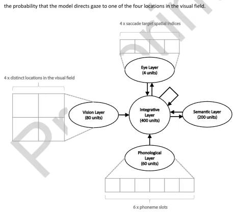
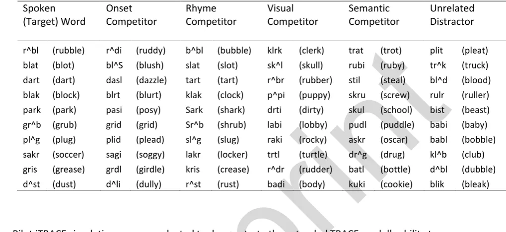
(12) 1. et al. (2013) 1. An overview of the implementation is provided below, for a full description of the. 2. motivation for and structure of the model, refer to Smith et al. (2013).. 3. Table 1: Table presents data recorded in the Visual World Paradigm that the MIM has previously been. 4. demonstrated to capture (Smith, Monaghan & Huettig, 2013, 2014) Study. Scene Item 1. Item 2. Target. Onset. Dahan & Tanenhaus (2005). Target. Visual. Rhyme. Item 4 Distractor. Distractor. Distractor. pr in. Allopenna et al. (1998). Item 3. t. Authors (year). Huettig & Altmann (2007). Visual. Distractor. Distractor. Distractor. Yee & Sedivy (2006). Target. Semantic. Distractor. Distractor. Huettig & Altmann (2005). Semantic. Distractor. Distractor. Distractor. Mirman & Magnuson (2009)a. Target. Near Semantic. Far Semantic. Distractor. Huettig & McQueen (2007)b. Onset. Semantic. Visual. Distractor. Notes: Item 1-4 indicate the relationship of each of the four objects presented in the visual display of each study. 6. to the spoken target word. Observed competitor effects are indicated in bold type. Onset = phonological onset. 7. competitor; Rhyme = phonological rhyme competitor; Visual = visual competitor; Semantic = semantic. 8. competitor.. 9. a. 10. b. 11. 2.1.1. Architecture. 12. The MIM utilises the parallel distributed processing framework (see Rumelhart, McClelland & the PDP. 13. Research Group, 1986; Rogers & McClelland, 2014). The network consists of layers of processing units. 14. connected via weighted connections. The architecture of the model is displayed in Figure 1. A layer of. 15. 80 units defines the visual layer. This layer provides input of visual information to the network from. e-. 5. Pr. Near and Far semantic competitors presented on separate trials Experiment 1. Model used within this study replicates the ‘noisy learning environment’ implementation described within Smith, Monaghan & Huettig (2013).. 1. 11.

(13) four locations (each represented by 20 units) in the visual field. A layer of 60 units provides input of. 2. phonological information to the network. This layer is divided into six phoneme slots, with each slot. 3. consisting of 10 units each sensitive to a specific phonological property of an utterance at a specific. 4. temporal location. Units in both phonological and visual layers are fully connected in a forward. 5. direction to a central integrative layer. The integrative layer consisted of 400 units and is fully self-. 6. connected. The integrative layer is also fully connected to both a semantic layer and an eye layer, in. 7. both forward and backward directions. The semantic layer consists of 200 units each of which are. 8. sensitive to a specific semantic property. The eye layer consists of four units with each unit encoding. 9. the probability that the model directs gaze to one of the four locations in the visual field.. Pr. e-. pr in. t. 1. 10 11 12. Figure 1: Architecture of the multimodal integration model of language mediated visual attention. 2.1.2. Representations 12.

(14) 24 artificial corpora were constructed, with each used to train and test a single simulation run of the. 2. model, this ensured that relationships within and between modalities were controlled. Each corpus. 3. consisted of 200 words, with each word assigned a unique phonological, semantic and visual. 4. representation. All words within the corpus were six phonemes in length. A phoneme inventory. 5. consisting of 20 phonemes was constructed, with each phoneme represented by a unique 10 unit. 6. binary phonological feature vector. Each phonological feature was assigned with p(active) = 0.5.. 7. Phonological representations were constructed by pseudo randomly sampling a unique sequence of. 8. six phonemes from the phoneme inventory to create each word. Controls ensured no more than 2. 9. consecutive phonemes were shared between words (other than in the case of phonological rhyme. 10. competitors, see Table 2). Visual representations were unique 20 unit binary feature vectors, with. 11. each unit representing the presence or absence of a specific visual feature. Visual features were. 12. assigned with p(active) = 0.5. Semantic representations by contrast were sparsely distributed, with. 13. each word pseudo-randomly assigned a unique set of eight semantic features from a possible 200. A. 14. maximum of 1 semantic property was shared between items (other than in the case of semantic. 15. competitors where 4 properties were shared, see Table 2).. 16. Table 2: Details of relationships between targets, competitors and unrelated distractors embedded. 17. within artificial corpora.. Pr. e-. pr in. t. 1. Constraint. Cosine. (Features shared with target). Distance. Representation. Item Type. Phonological. Competitor. Final 3 of 6 phonemes. 0.259. Unrelated. Max. 2 consecutive phonemes. 0.496. Competitor. 4 of 8 semantic features. 0.500. Unrelated. Max. 1 semantic feature. 0.959. Competitor. Min. 5 of 10 visual features. 0.264. Unrelated. Features shared with p = (0.5). 0.506. Semantic. Visual. 18 13.

(15) Constructing artificial corpora ensured that we controlled the relations between the stimuli,. 2. specifically the relationships between competitors, targets and unrelated items. Embedded within the. 3. corpus were 20 sets of items that shared increased overlap in either semantic, visual or phonological. 4. dimensions. Each of the 20 sets contained a target, a phonological competitor, a semantic competitor. 5. and a visual competitor. Each ‘target’ word shared the final three of its six phonemes with the. 6. phonological rhyme competitor. As Table 2 indicates, overlap between phonologically unrelated items. 7. was small, with a mean 0.31 phonemes overlapping between words. Similarly, in natural language. 8. vocabularies, overlap is small, for the 9374 words of length 6 phonemes in English from the CELEX. 9. database, the mean overlap in phonemes was .39 between any pair of words. Semantic competitors. 10. were defined by sharing four of their eight semantic features with the target and visual competitors a. 11. minimum of 5 of their 10 visual features with the target. This ensured that in all dimensions the. 12. distance between competitor and target was half that between competitor and an unrelated item (see. 13. Table 2).. 14. 2.1.3. Training. 15. In training the model we assume that individuals learn associations between representations of an. 16. item across modalities through repeated, simultaneous exposure to multiple representational forms. 17. of an item. Networks were trained on four cross modal mapping tasks: object recognition; spoken. 18. word comprehension; speech motivated orientation; and semantically motivated orientation. Time in. 19. the model was represented by the flow of information across weighted connections between units in. 20. the network. Each training task ran for 14 time steps (ts).. 21. For object recognition tasks, four items were randomly selected from the training corpus and their. 22. visual representations presented to the four visual input slots within the visual layer (ts = 0). One of. 23. the four items was then randomly selected as a target and the eye gaze layer unit corresponding to. 24. the location of the target’s visual representation in the visual layer was fully activated (ts = 0). Visual. 25. input and eye gaze layer activation remained fixed across the training trial while random time invariant. Pr. e-. pr in. t. 1. 14.

(16) noise was provided as an input to the phonological layer. At time step 3 until the end of the trial (ts =. 2. 14) the semantic representation of the target was presented to the semantic layer and error back. 3. propagated.. 4. Spoken word comprehension tasks involved randomly selecting an item from the corpus as a target.. 5. The phonological representation of the target item was then over time (from ts = 0) presented to the. 6. phonological layer of the network, with an additional phoneme presented at each subsequent time. 7. step. To simulate exposure to noise in the auditory input within the learning environment the binary. 8. value of each unit within the phonological representation of the target was switched (i.e. 0 -> 1 or 1 -. 9. > 0) with p = 0.2 (see Smith et al., 2013). Random time invariant noise was presented as input to the. 10. visual layer during such trials, while no constraints were placed on eye layer activity. At time step 5. 11. the semantic representation of the target was presented to the semantic layer and error. 12. backpropagated until the end of the training trial (ts = 14).. 13. For phonological orientation tasks, four items were randomly selected and their visual representations. 14. presented as input to the visual layer (ts 0 – 14). One of the four items was randomly selected as a. 15. target. The target’s phonological representation was then presented over time (from ts = 0) as input. 16. to the phonological layer, with an additional phoneme presented at each subsequent time step. As in. 17. word comprehension tasks, to simulate exposure to noisy auditory signals in the learning environment. Pr. e-. pr in. t. 1. 18. the value of each unit in the target’s phonological representation was switched with p = 0.2. No. 19. constraints were placed on activity in the semantic layer. At time step 5 (point of phonological. 20. disambiguation) the eye layer unit corresponding to the location of the target’s visual representation. 21. was required to be fully activated and error backpropagated until the end of the training trial (ts = 14).. 22. Finally, semantic orientation trials followed a similar procedure. Again four items were randomly. 23. selected from the corpus and their visual representations presented as input to the visual layer (ts 0-. 24. 14). One of these four items was randomly selected as a target and its semantic representation. 25. presented to the semantic layer (ts 0 - 14). Random time invariant noise was presented to the 15.

(17) phonological layer throughout this trial. At time step 2 the eye layer unit that corresponded to the. 2. location of the visual representation of the target was required to be fully activated and error. 3. backpropagated until the end of the training trial (ts = 14).. 4. We assume that speech motivated orientation is less frequent in the learning environment than object. 5. recognition, spoken word comprehension and semantically motivated orientation and therefore this. 6. task was four times less likely to occur during training. Given this constraint training tasks were. 7. randomly interleaved.. 8. Simulations were conducted using Mikenet version 8.0 developed by M. W. Harm. 9. (www.cnbc.cmu.edu/~mharm/research/tools/mikenet/), a collection of libraries written in the C. 10. programming language for implementing and training connectionist networks. Connection weights. 11. within the model were initialised with random weights from the uniform distribution [-0.1, 0.1].. 12. Recurrent backpropagation (learning rate = 0.05) was used during training to adjust weights within. 13. the network using the continuous recurrent backpropagation through time training algorithm. 14. provided in Mikenet (crbp.c) which implements Pearlmutter (1989). Unit activation was calculated. 15. using a logistic activation function and sum squared error was used to calculate error. Time within the. 16. network was modelled using an integration constant of 0.25 with 14 samples during training and 30. 17. samples during test simulations of visual world conditions (Time steps of test trials are reported. Pr. e-. pr in. t. 1. 18. relative to word onset [i.e. word onset = ts 0]). Additional time was provided during test simulations. 19. to allow insight into the time course of interaction of information between modalities in the model.. 20. All other parameters were set to the default values implemented in Mikenet version 8.0. A total of. 21. 1,250,000 training trials were performed before the model was exposed to test conditions. Once. 22. trained all networks performed spoken word comprehension and object recognition tasks accurately. 23. (i.e. semantic layer activity was closest in terms of cosine distance to that of the target) for all items. 24. in the training corpus. On orientation tasks the model looked to the location of the target on at least. 25. 3 of 4 test trials for 99.75% (speech motivated orientation) and 100% (semantically motivated. 16.

(18) orientation) of items. 24 simulation runs of the model were performed, each initiated with a different. 2. initial random seed. Sections 2.2 and 2.3 report mean behaviour calculated across all 24 simulation. 3. runs of the model.. 4. 2.2. Simulation 1: Simulating effects of phonological rhyme overlap. 5. Previous visual world studies demonstrate that phonological rhyme overlap exerts an influence on. 6. language mediated visual attention under conditions in which phonology provides the only dimension. 7. in which auditory and visually presented stimuli are related. We first examine the model’s sensitivity. 8. to phonological rhyme overlap when presented with scenes containing a single rhyme competitor and. 9. three unrelated items.. pr in. t. 1. 2.2.1. Procedure. 11. Test trials lasted a total of 30 time steps (ts -5 to 24). The visual representations of four objects were. 12. presented to the visual layer at trial onset (ts = -5) and remained present until the end of the trial (ts. 13. = 24). Three of the items were unrelated to the upcoming target word, i.e., controlled low level of. 14. overlap with the target in visual, semantic or phonological dimensions (see Table 2). The fourth item. 15. was a phonological rhyme competitor in that it shared the final three phonemes of its phonological. 16. representation with the upcoming target word. The network was then free to cycle for five time steps. 17. (ts -5 to -1) to allow pre-processing of the visual information (replicating previous visual world studies. Pr. e-. 10. 18. in which a preview of the visual display is often provided, see Huettig & McQueen, 2007). At time step. 19. 0 the phonological representation of the target word began to unfold with an additional phoneme. 20. presented at each subsequent time step to the phonological layer. Unlike in training, no noise was. 21. applied to the phonological input of the target representation. Activation in the eye layer was. 22. recorded throughout the trial. The location in the visual field fixated by the model at a given time point. 23. was recorded as the location associated with the most activated unit in the eye layer at the given point. 24. in time. This procedure was followed for all rhyme competitor and target pairs within the corpus (n =. 17.

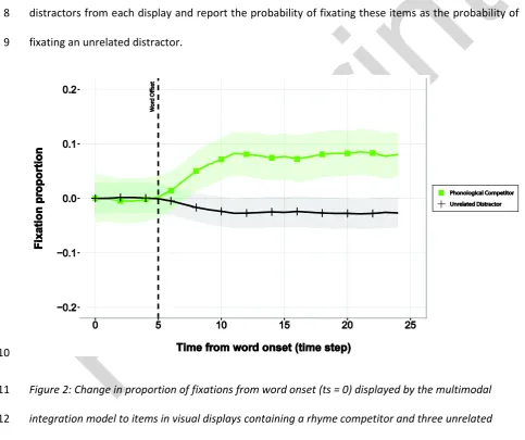
(19) 20) with rhyme competitors and distractors tested in all possible combinations of location (n = 24). 2. resulting in a total of 480 test trials per simulation run of the model.. 3. 2.2.2. Results. 4. Figure 2 presents the change from word onset (ts = 0) in the probability of fixating rhyme competitors. 5. and unrelated distractors. To allow us to compare the same items across conditions (i.e. difference in. 6. probability of fixating a rhyme competitor compared to an unrelated distractor in the presence or. 7. absence of visual and semantic competitors) we randomly selected one of the three unrelated. 8. distractors from each display and report the probability of fixating these items as the probability of. 9. fixating an unrelated distractor.. Pr. e-. pr in. t. 1. 10. 11. Figure 2: Change in proportion of fixations from word onset (ts = 0) displayed by the multimodal. 12. integration model to items in visual displays containing a rhyme competitor and three unrelated. 13. distractors. Shaded areas define 95% confidence intervals.. 14. To examine whether looks to phonological rhyme competitors exceeded looks to unrelated. 15. distractors, for analysis we divided the 30 time step test trial into five equal time windows. We then. 18.

(20) compared fixation behaviour displayed by the model in the baseline time window (ts -5 to 0), the 6. 2. time steps from trial onset to word onset, to fixation behaviour displayed by the model in each of the. 3. four time windows post word onset (ts 1 - 6; ts 7 - 12; ts 13 - 18; ts 19 - 24). For each window we. 4. calculated the empirical log odds of fixating each category of object within the display (i.e., rhyme. 5. competitor, unrelated distractor). This measure avoids issues arising from calculating estimates based. 6. on proportional data (see Jaeger, 2008). Our dependent measure was the difference between the log-. 7. odds of fixating the phonological rhyme competitor and the log-odds of fixating the unrelated. 8. distractor. This reflects the difference in fixation of competitor objects as a consequence of. 9. representational overlap. We used linear mixed effect models to examine whether gaze differed as a. 10. consequence of phonological rhyme overlap in the time windows post word onset relative to levels of. 11. fixation in the baseline time window. Mixed effects model analysis was performed using the R (version. 12. 3.1.0; R Development Core Team, 2009) libraries lme4 (version 1.1-6; Bates, Maechler, Bolker &. 13. Walker, 2015). The model constructed applied the maximal random effect structure (Barr, Levy,. 14. Scheepers, & Tily, 2013), the fixed effect time window and random effects of model simulation run (n. 15. = 24) and item (n = 20), including random intercepts and slopes for time window both by simulation. 16. run and item. To derive p-values we assumed t-values were drawn from a normal distribution (Barr,. 17. 2008).. 18. Examining parameter estimates within the model revealed that in the first time block that followed. 19. word onset (ts 1 - 6) phonological rhyme competitors were fixated marginally less than unrelated. 20. distractors relative to the baseline time window (β = -0.082, t = -1.72, p = 0.086). In the second time. 21. window (ts 7 - 12), this trend reversed with rhyme competitors fixated more than unrelated items (β. 22. = 0.385, t = 3.02, p = 0.003). This increased rhyme effect remained in the final two time windows ts 13. 23. - 18 (β = 0.486, t = 3.68, p < 0.001) and ts 19 - 24 (β = 0.480, t = 3.53, p < 0.001).. 24. 2.2.3. Summary. Pr. e-. pr in. t. 1. 19.

(21) Results of Simulation 1 demonstrate that the MIM displays sensitivity to phonological rhyme overlap. 2. when presented with scenes containing a single rhyme competitor amongst unrelated items with. 3. effects predicted to emerge post word offset. This replicates previous behavioural findings that. 4. language mediated eye gaze is sensitive to phonological rhyme overlap between spoken target words. 5. and visually displayed objects (Allopenna et al., 1998; Huettig & McQueen, 2012; McQueen & Viebahn,. 6. 2007). Further, the model demonstrates that a fully interactive alignment model of spoken word. 7. processing (MIM) is able to generate phonological rhyme effects (Magnuson, Tanenhaus & Aslin,. 8. 2000; Magnuson et al., 2003; Smith, Monaghan & Huettig, 2013; cf. Allopenna et al., 1998).. 9. 2.3. Simulation 2: Simulating effects of multimodal competition. pr in. t. 1. A second set of simulations examined the relative influence and timing of effects of phonological. 11. rhyme, semantic and visual overlap on eye gaze within the MIM and the effect of additional. 12. competition from visual and semantic competitors on phonological rhyme effects that were exhibited. 13. in Simulation 1.. 14. 2.3.1. Procedure. 15. Simulation 2 followed the same training and testing procedure as outlined for Simulation 1 (see. 16. section 2.2.1), however test scenes now contained a rhyme competitor, a semantic competitor, a. 17. visual competitor and an unrelated distractor (scenes contained the same rhyme competitor and. Pr. e-. 10. 18. unrelated distractor pairs as analysed in section 2.2.2). Again simulations were run for all target and. 19. competitor sets embedded within the corpus (n = 20) with sets tested in all possible combinations of. 20. location (n=24) resulting in a total of 480 test trials per simulation run. Results report the probability. 21. of fixating an item at any given time point, this is taken as the proportion of trials on which at that. 22. given point in the trial the eye layer unit associated with location of the given object is the most. 23. activated unit in the eye layer.. 24. 2.3.2. Results. 20.

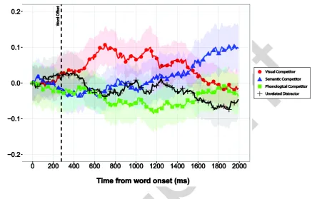
(22) The change in the probability of fixating each category of item (i.e., rhyme competitor, semantic. 2. competitor, visual competitor and unrelated distractor) from word onset is presented in Figure 3.. 3. Visual inspection suggests a rapid increase in fixation of visual competitors shortly after word onset,. 4. with increased fixation of semantic competitors emerging slightly later and at lower levels. Fixation of. 5. phonological rhyme competitors also appears to depart from unrelated distractor levels however this. 6. appears later than semantic and visual competitors and is a weaker effect.. 7. Figure 3: Change in the proportion of fixations from word onset displayed by the multimodal. Pr. 8. e-. pr in. t. 1. 9. integration model to items in visual displays containing a rhyme competitor, a visual competitor, a. 10. semantic competitor and an unrelated distractor. Shaded areas define 95% confidence intervals.. 11. We used the same procedure for analysis of Simulation 2 as used in Simulation 1. However, scenes in. 12. Simulation 2 contained three competitors rather than a single competitor in Simulation 1. We. 13. therefore compared separately for each category of competitor (visual, semantic, rhyme) the. 14. difference in empirical log odds of fixating the given competitor and the unrelated distractor in each. 15. time window post word onset (ts 1 - 6, ts 7 - 12, ts 13 - 18, ts 19 - 24) to the difference observed in the. 16. baseline time window (ts -5 to 0), the 6 time steps from trial onset to word onset. For analysis we used 21.

(23) linear mixed effect models with a fixed effect of time window and random effects of model simulation. 2. run (n = 24) and item (n = 20), including random intercepts and slopes for time window both by. 3. simulation run and item.. 4. This analysis revealed that phonological rhyme, visual, and semantic competitors were fixated above. 5. unrelated distractor levels in windows ts 7 - 12 (rhyme: β = 0.284, t = 2.90, p = 0.004; visual: β = 0.727,. 6. t = 8.27, p < 0.001; semantic: β = 0.666, t = 6.99, p < 0.001), ts 13 - 18 (rhyme: β = 0.289, t = 2.90, p =. 7. 0.004; visual: β = 1.265, t = 12.2, p < 0.001; semantic: β = 1.107, t = 9.41, p < 0.001) and ts 19 - 24. 8. (rhyme: β = 0.345, t = 3.60, p < 0.001; visual: β = 1.311, t = 14.80, p < 0.001; semantic: β = 1.138, t =. 9. 9.01, p < 0.001). While in the first time block post word onset (ts 1 - 6) there was no difference between. 10. competitors and unrelated distractors (rhyme: β = 0.014, t = 0.244, p = 0.807; visual: β = -0.045, t = -. 11. 0.864, p = 0.388; semantic: β = 0.003, t = 0.052, p = 0.959).. 12. To examine whether the magnitude of competitor effects differed we used the same analysis. 13. technique to test in each of the post word onset time windows (ts 1 - 6, ts 7 - 12, ts 13 - 18, ts 19 - 24). 14. relative to the baseline time window (6 time steps prior to word onset, ts -5 to 0) whether: the log. 15. odds of fixating the visual competitor differed from the log odds of fixating the semantic competitor;. 16. the log odds of fixating the visual competitor differed from the log odds of fixating the rhyme. 17. competitor; and the log odds of fixating the semantic competitor differed from the log odds of fixating. Pr. e-. pr in. t. 1. 18. the rhyme competitor. This analysis did not reveal a significant difference between fixation of the. 19. semantic competitor compared to fixation of visual competitors in any time window relative to the. 20. baseline window (ts 1 - 6: β = -0.048, t = -0.765, p = 0.444; ts 7 - 12: β =0.061, t = 0.585, p = 0.558; ts. 21. 13 - 18: β = 0.159, t = 1.251, p = 0.211; ts 19 - 24: β = 0.173, t = 1.33, p = 0.185). Visual and Semantic. 22. competitors were however fixated more than rhyme competitors relative to baseline levels in all time. 23. windows post word onset other than ts 1 - 6 (Semantic vs. Rhyme: ts 1 - 6: β = -0.011, t = -0.204, p =. 24. 0.838; ts 7 - 12: β = 0.383, t = 3.92, p < 0.001; ts 13 - 18: β = 0.818, t = 7.39, p < 0.001; ts 19 - 24: β =. 22.

(24) 0.793, t = 7.52, p < 0.001; Visual vs. Rhyme: ts 1 - 6: β = -0.059, t = -1.16, p = 0.248; ts 7 - 12: β = 0.443,. 2. t = 3.66, p < 0.001; ts 13 - 18: β = 0.976, t = 7.55, p < 0.001; ts 19 - 24: β = 0.966, t = 7.74, p < 0.001).. 3. Finally, using mixed effects models we analysed whether the difference in empirical log odds of. 4. fixating the phonological rhyme competitor and empirical log odds of fixating the unrelated distractor. 5. differed between Simulation 1 and Simulation 2. Did the presence of visual or semantic competitors. 6. influence the magnitude of the phonological rhyme effect? This was performed using a model with. 7. fixed effects of time window and scene (Scene 1: rhyme competitor and unrelated distractors only;. 8. Scene 2: rhyme competitor, semantic competitor, visual competitor and unrelated distractor) and. 9. random effects of model simulation run (n = 24) and item (n = 20), including random intercepts and. 10. slopes for both time window and scene both by simulation run and item. Analysing the rhyme effect. 11. in the baseline time window (6 time steps prior to word onset, ts -5 to 0) in relation to that observed. 12. in ts 1 - 6 revealed no main effect of time window (β = -0.034, t = -0.69, p = 0.490), although there was. 13. a marginal main effect of scene (β = 0.107, t = 1.67, p = 0.096) and a marginal interaction between. 14. time window and scene (β = 0.096, t = 1.89, p = 0.059) suggesting that the presence of visual and. 15. semantic competitors increased the rhyme effect marginally in this early window. By contrast. 16. comparing the rhyme effect observed in the baseline time window to that observed in later time. 17. windows ts 7 - 12, ts 13 - 18 and ts 19 - 24 revealed for all later windows a main effect of time window. 18. (ts 7 - 12: β =0.334, t = 3.15, p = 0.002; ts 13 - 18: β = 0.388, t = 3.62, p < 0.001; ts 19 - 24: β = 0.413, t. 19. = 3.82, p < 0.001), no main effect of scene (ts 7 - 12: β = 0.008, t = 0.049, p = 0.868; ts 13 - 18: β = -. 20. 0.039, t = -1.16, p = 0.248; ts 19 - 24: β = -0.009, t = -0.244, p = 0.807) and a significant negative. 21. interaction term between time window and scene (ts 7 - 12: β =-0.102, t = -2.27, p = 0.023; ts 13 - 18:. 22. β = -0.197, t = -4.32, p < 0.001; ts 19 - 24: β = -0.135, t = -2.91, p = 0.004) demonstrating that the. 23. presence of visual and semantic competitors reduced the rhyme effect in later time windows.. 24. 2.4.. Pr. e-. pr in. t. 1. Summary. 23.

(25) In summary the MIM predicts that all items that overlap with the spoken target word in terms of visual. 2. properties, semantic properties or phonological rhyme will be fixated above unrelated distractor. 3. levels. All effects emerged gradually post word offset and within the same time window post word. 4. offset (ts 7 - 12). With regard to behavioural data, the MIM with interactivity at all stages of processing,. 5. predicts that visual and semantic effects will be of a similar magnitude, although beta estimates were. 6. numerically higher in all post word offset time windows for visual competitors. In relation to rhyme. 7. competitor effects both visual and semantic competitor effects were predicted to be far greater, with. 8. differences emerging shortly after word onset and increasing across the remainder of the test window.. 9. Comparisons of rhyme effects observed in the presence (Simulation 2) and absence (Simulation 1) of. 10. visual competitors generate the prediction that the presence of visual and semantic competitors will. 11. weaken the effect of phonological rhyme overlap on fixation behaviour in time windows post word. 12. offset.. 13 15. 3. Simulating the effects of multimodal competition on phonological rhyme overlap in a lexical level cascading model of language mediated visual attention. 16. In this section we detail the predictions generated by a cascaded architecture in which activation from. 17. visual and sematic levels connects with phonological activation at the lexical level as simulated by the. 18. word level nodes of the TRACE (McClelland & Elman, 1986; Spivey, 2007) model. The architecture of. pr in. e-. Pr. 14. t. 1. 19. our implementation of this extended TRACE model is presented in Figure 4. This model contrasts with. 20. the MIM in terms of when information between modalities is permitted to interact. The predictions. 21. of each model are then tested using the behavioural data of Experiments 1 and 2, below.. 22. 3.1. Implementing an influence of cascading multimodal information into the TRACE. 23. model of spoken word recognition. 24.

(26) Figure 4: Architecture of the extended multimodal TRACE model.. Simulations were performed using jTRACE (Strauss, Harris, & Magnuson, 2007). All parameters were. Pr. 3. pr in. t 2. e-. 1. 4. set to default values other than the following subset that were manipulated to simulate cascading. 5. activation from visual and semantic levels entering the TRACE hierarchy to be integrated with. 6. phonological information at the lexical level. The resting level of nodes at the lexical level of the TRACE. 7. hierarchy can be affected in jTRACE by manipulating the frequency resting state (see Dahan,. 8. Magnuson and Tanenhaus, 2001) and priming resting state parameters. These parameters alter lexical. 9. level node activation as determined by equation 1.. 10. 𝑟𝑟𝑖𝑖 = 𝑅𝑅 + 𝑠𝑠𝑓𝑓 [ 𝑙𝑙𝑙𝑙𝑙𝑙10 (𝑐𝑐 + 𝑓𝑓𝑖𝑖 ) ] + 𝑠𝑠𝑝𝑝 [ 𝑙𝑙𝑙𝑙𝑙𝑙10 (𝑐𝑐 + 𝑝𝑝𝑖𝑖 ) ]. (1). 25.

(27) 1 2 3. frequency resting level scaling constant, c is a constant that ensures the value within parenthesis is. greater than 0, sp is the priming resting level scaling constant, fi is the frequency of item i, pi is the. 5. priming value for item i. In our simulations fi and pi were used to represent the relative level of. 6. thus represents the relative magnitude of activation cascading from visual and semantic levels to. 7. activate the node representing item i at the lexical level. A positive linear function applied to 𝑠𝑠𝑓𝑓 and. 8. representational overlap at visual and semantic levels between a given item and the target word, and. 𝑠𝑠𝑝𝑝 ensured that cascading activation from visual and semantic levels ramped up over time as. t. 4. In equation 1 ri is the resting activation for unit i, R is the default resting level for all units, sf is the. activation of associated representations in these modalities increased. We implemented the. 10. assumption that time is required for activation to cascade between modalities. This was done by. 11. ensuring that activation generated at visual and semantic levels by overlap in cascading activation. 12. from visual and auditory signals began influencing activation at the lexical level within TRACE six time. 13. steps after the onset of the spoken target word (equal to the time taken for a single phoneme to. 14. unfold).. 15. Pilot simulations explored the parameter space in order to identify a range of values for 𝑓𝑓𝑖𝑖 , 𝑝𝑝𝑖𝑖 , 𝑠𝑠𝑓𝑓 and. e-. 17. 𝑠𝑠𝑝𝑝 able to generate behaviour consistent with that recorded in the data sets detailed in Table 1, which. 18. demonstrated an ability to replicate (see appendix B for further details of pilot simulations conducted. 19. with the extended TRACE model that demonstrate the model’s ability to generate visual and semantic. 20. competitor effects in both the presence and absence of the target item in addition to the complex. 21. time course of fixation behaviour generated by multi-competitor scenes as observed in Allopenna et. 22. al. (1998) [phonological onset competitor, phonological rhyme competitor & target] and Huettig &. 23. McQueen (2007) [phonological onset competitor, visual competitor & semantic competitor].. 24. In our initial parameterisation of TRACE we assume that the resting state of nodes at the lexical level. 25. corresponding to items in the visual display is equal at word onset. As the spoken target word unfolds. a fully interactive parallel processing system (MIM: Smith et al., 2013; 2014) has previously. Pr. 16. pr in. 9. 26.

(28) this increases activation of phonologically related words. Activation of such words at the lexical level. 2. then cascades to activate the visual and semantic properties of these items. At the same time,. 3. information relating to the visually displayed items is also cascading from visual levels to constrain. 4. activation of the visual and semantic properties. Thus at the lexical level, post target word onset,. 5. cascading activation from visual and semantic levels should increase activation of items that share. 6. properties at the visual and semantic level that are supported both by the incoming visual and auditory. 7. signal.. 8. In our simulations we therefore aimed to model the change from word onset in the nature of. 9. activation cascading from visual and semantic levels to affect lexical level activation. This is performed. 10. by manipulating parameters 𝑓𝑓𝑖𝑖 , 𝑝𝑝𝑖𝑖 , 𝑠𝑠𝑓𝑓 and 𝑠𝑠𝑝𝑝 in jTRACE. In these simulations we use 𝑓𝑓𝑖𝑖 to define the. pr in. t. 1. 11. magnitude of the increase, relative to word onset, of activation cascading from visual levels to activate. 12. the lexical level node corresponding to item i. 𝑝𝑝𝑖𝑖 is used to define the magnitude of the increase,. 14 15 16 17. relative to word onset, of activation cascading from semantic levels to activate the lexical level node corresponding to item i. 𝑠𝑠𝑓𝑓 is a scaling factor defining the level of influence of cascading activation. e-. 13. from visual levels on activation of all lexical level nodes. 𝑠𝑠𝑝𝑝 is a scaling factor defining the level of. influence of cascading activation from semantic levels on all lexical level nodes. We determined the relative values of parameters𝑓𝑓𝑖𝑖 , 𝑝𝑝𝑖𝑖 for each category of item (target, visual competitor, semantic. competitor, phonological onset competitor, phonological rhyme competitor, unrelated distractor) by. 19. first assigning values to the items that overlapped maximally and minimally with the shared auditory. 20. and visual signals, the target item and the unrelated distractor.. 21. In target present scenes the lexical level node of the target item is supported maximally by information. 22. cascading from phonological processing levels, given that its complete phonological form is present in. 23. the auditory input signal. Similarly, cascading activation from visual and semantic levels to lexical level. 24. nodes can also be assumed to increase maximally post word onset as the target's visual and semantic. 25. properties are likely fully activated by activation cascading both top down from lexical levels and. Pr. 18. 27.

(29) 1. bottom up from visual levels given the presence of the target's full visual form in the visual input. We. 2. therefore assigned the ceiling value of 1000 for parameters 𝑓𝑓𝑖𝑖 and 𝑝𝑝𝑖𝑖 (see Dahan, Magnuson, &. 3. Tanenhaus, 2001) for target items when present in the display. Conversely, although the visual input. 4. signal contains the visual form of the unrelated distractor, there is no additional support for this item. 5. in the auditory signal. Thus, from word onset, there should be no increase in activation of visual or. 6. semantic properties of the unrelated distractor. For this reason parameters 𝑓𝑓𝑖𝑖 and 𝑝𝑝𝑖𝑖 were assigned a were also assigned a value of 0 for both parameters 𝑓𝑓𝑖𝑖 and 𝑝𝑝𝑖𝑖 .. t. 8. value of 0 for unrelated distractors. All items in the corpus that were not present in the visual display. pr in. 7. 9. By contrast competitor items each receive additional support from cascading activation initiated post. 10. word onset. In the case of the visual competitor, the auditory signal increases activation of the target's. 11. visual properties, which are shared with the visual competitor, thus we assume this also increases the. 12. amount of activation cascading from visual levels to activate the visual competitor at the lexical level.. 13. We therefore assigned visual competitors an 𝑓𝑓𝑖𝑖 value of 500 (𝑝𝑝𝑖𝑖 = 0), half that of the target item.. Similarly, for semantic competitors, activation of the semantic properties corresponding to the target. 15. word, which are also shared with the semantic competitor, are assumed to increase activation. 16. cascading from semantic levels to activate the semantic competitor at the lexical level. Therefore, 𝑝𝑝𝑖𝑖. 17. was assigned a value of 500 for all semantic competitors (𝑓𝑓𝑖𝑖 = 0), half that of the target. These ratios were motivated by the results of behavioural rating studies (see Table 5) and Huettig & McQueen. Pr. 18. e-. 14. 19. (2007, Table 2) which showed that the ratio of the similarity between unrelated distractor and target. 20. compared to visual or semantic competitor and target was approximately 0.5 (Huettig & McQueen,. 21. 2007: Visual/Unrelated = 0.51, Semantic/Unrelated = 0.50; Smith, Monaghan & Huettig, current study:. 22. Visual/Unrelated = 0.41, Semantic/Unrelated = 0.47).. 23. Given such an architecture, we can also assume that cascading activation from visual and semantic. 24. levels also increases post word onset, relative to unrelated distractor levels, for both phonological. 25. onset and phonological rhyme competitors should they be present in the visual display. As discussed. 28.

(30) in section 1.1, previous applications of TRACE to model visual world data (e.g. Allopenna et al. 1998). 2. demonstrated that items that share phonological properties in their rhyme or onset with the target. 3. word are activated above unrelated items at the lexical level. Within this architectural framework we. 4. therefore assume that this activation also then cascades to activate the visual and semantic properties. 5. of such phonologically related items, properties that are also supported by cascaded activation from. 6. the visual input given the presence of their visual form in the visual display. Further, these previous. 7. simulations also demonstrate that the location (onset or rhyme) of the phonological overlap will. 8. determine the magnitude and onset of this cascading activation.. 9. Allopenna et al. (1998) shows that activation of lexical level nodes for phonological onset competitors. 10. increases at a rate identical to targets, prior to the speech signal disambiguating between the two. 11. items. Following disambiguation, activation of the onset competitor at the lexical level decreases. 12. rapidly. Therefore, to simulate such conditions in the extended TRACE model, for scenes in which. 13. onset competitors are present, in the period prior to phonological disambiguation the onset. 14. competitors parameters are 𝑓𝑓𝑖𝑖 and 𝑝𝑝𝑖𝑖 = 1000. In the period post disambiguation parameters 𝑓𝑓𝑖𝑖 and 𝑝𝑝𝑖𝑖. e-. pr in. t. 1. = 0. By contrast activation of the lexical level node corresponding to the rhyme competitor only. 16. increases above unrelated distractor levels once phonological information carried in the rhyme. 17. becomes available. Further the overall level of activation reached by the rhyme competitor is lower. 18. than that obtained by the onset competitor as earlier activation of onset competitors inhibits later. 19. activation of the rhyme competitor. However, as there is activation of the rhyme competitor at the. 20. lexical level above unrelated distractor levels, we can assume this additional activation cascades to. 21. activate semantic and visual properties associated with the rhyme competitor. If the rhyme. 22. competitor is present in the visual scene, this cascading activation to visual and semantic levels will be. 23. supported by cascading activation initiated by the presence of the rhyme competitor’s visual form in. 24. the visual signal. We therefore assign parameters 𝑓𝑓𝑖𝑖 and 𝑝𝑝𝑖𝑖 = 50 for rhyme competitors so as to. Pr. 15. 25. simulate the small levels of activation cascading from visual and semantic levels to influence activation. 26. at the lexical level. We believe a value of 5% of the target’s activation is a conservative estimate given 29.

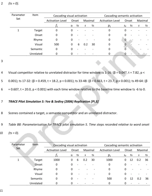
(31) 1. that in Allopenna et al. (1998) the lexical level nodes corresponding to rhyme competitors are at their. 2. peak activated to approximately 10% the level of the target item. Note that increasing this value of 𝑓𝑓𝑖𝑖. 3 4 5. and 𝑝𝑝𝑖𝑖 for rhyme competitors would have the effect of further increasing the activation of the phonological competitor.. By applying a linear function to scaling factors 𝑠𝑠𝑓𝑓 and 𝑠𝑠𝑝𝑝 we controlled the onset and level of activation. cascading over time from visual and semantic levels, respectively. For all items other than rhyme. 7. competitors activation of their lexical level nodes due to cascading activation from visual levels. 8. increased from 6 time steps post word onset as scaling factors 𝑠𝑠𝑓𝑓 increased linearly from 0 to 0.2 over. pr in. t. 6. 9. the course of 24 time steps (number of time steps required for full phonological form of target word. 10. to unfold). Activation from semantic levels increased in an identical manner but with the onset delayed. 11. by 6 time steps in order to simulate a delayed effect of semantic activation (see Huettig & McQueen,. 12. 2007). For rhyme competitors activation entering the lexical level from both visual and semantic levels. 13. increased 12 time steps post word onset, with scaling factors 𝑠𝑠𝑓𝑓 and 𝑠𝑠𝑝𝑝 increased linearly from 0 to. 0.2 over the course of 24 time steps. Thus, the onset of such increased activation occurs six time steps. 15. after the onset of the first phoneme that overlaps with the target word.. 16. A second parameterisation of the extended TRACE system was also tested. This second. 17. parameterisation aimed to maximise the likelihood of observing effects of visual and semantic. Pr. e-. 14. 18. competition on the rhyme effect. In this parameterisation, activation cascading from visual levels to. 19. influence lexical nodes occurred at the same time step as that cascading from semantic levels. In the. 20. case of rhyme competitors the onset of activation occurred 6 time steps later than all other items. The. 21. scaling constant determining the influence of semantic and visual activation (𝑠𝑠𝑓𝑓 and 𝑠𝑠𝑝𝑝 ) was also. 22. increased linearly as described above yet to an increased level of 0.5 (pilot studies explored values for. 23. 𝑠𝑠𝑓𝑓 and 𝑠𝑠𝑝𝑝 beyond this level yet this generated an increasingly worse fit to the data sets described in. 24. Table 1). In the second parameterisation of the system to maximise competition all related items. 30.

(32) 1. (target, onset competitor, rhyme competitor, semantic competitor, visual competitor) received. 2. feedback from visual and semantic levels, even though they may not be present in the visual display.. 3. As in previous studies that have applied TRACE to model visual world data, the Luce choice rule. 4. (Luce, 1959) was applied to raw lexical node activations for each item present in the visual display,. 5. the result of which was taken to represent the probability of fixating each displayed item.. 6. Table 3: Controls on TRACE stimuli. Visual Competitor Semantic Competitor. 7. Unrelated Distractor. M. SD. M. SD. 26.9. 11.1. 5.20. 30.0. 8.1. 33.2 30.2. Shared Phonemes. Phoneme Overlap. M. SD. M. SD. 2.09. 3.30. 0.46. 3.00. 0.00. 7.80. 3.76. 1.00. 0.63. 0.00. 0.00. 12.0. 6.20. 3.76. 0.80. 0.40. 0.00. 0.00. 6.4. 6.30. 2.97. 0.80. 0.60. 0.00. 0.00. pr in. Rhyme Competitor. Cohorts 2. t. Cohorts 1. We used the default corpus provided with jTRACE which was supplemented with additional words to. 9. create 10 distinct stimuli sets (see appendix table B1). Each set included a target word, a phonological. 10. onset competitor, a phonological rhyme competitor, a visual competitor, a semantic competitor and. 11. an unrelated distractor. All words were four phonemes in length. Rhyme competitors shared all but. 12. their initial phoneme with the target. Onset competitors shared their initial two phonemes with the. 13. target. Controls (see table 3) ensured that rhyme competitors, visual competitors and semantic. Pr. e-. 8. 14. competitors did not differ from unrelated distractors in their cohort density (t < 1.01, p > 0.32), while. 15. visual and semantic competitors did not differ from unrelated distractors in the number of phonemes. 16. shared with the target (Table 3, shared phonemes: t < 0.69, p > 0.49). Further visual competitors,. 17. semantic competitors and unrelated distractors did not have any shared phonemes in the same. 18. location as the target (see Table 3, phoneme overlap).. 19. 3.2. Simulating effects of phonological rhyme overlap in TRACE. 31.

(33) We used the extended TRACE model to first generate predictions for how fixation would be distributed. 2. towards objects in a scene that contained a single rhyme competitor accompanied by only unrelated. 3. items (i.e. conditions simulated in MIM in section 2.2).. 4. 3.2.1. Procedure. 5. Table 4: jTRACE parameterisations for simulations of word processing during exposure to visual. 6. scenes for Simulation 1 (Scene 1: rhyme competitor and unrelated distractors) and Simulation 2. 7. (Scene 2: rhyme competitor, visual competitor, semantic competitor and unrelated distractor). Time. 8. steps recorded relative to word onset (ts = 0). Item. P1. Target. pr in. Paramete r Set. t. 1. Cascading visual activation Activation Level (𝑓𝑓𝑖𝑖 ) Onset Maximal Scene Scene s 1 2 ts s ts f 0. 0. 0. -. -. -. 0. 0. 0. -. -. -. 0. 0. 0. -. -. -. 0. 0. 0. -. -. -. 50. 50. 0. 12. 0.2. 36. 50. 50. 0. 12. 0.2. 36. 0. 500. 0. 6. 0.2. 30. 0. 0. 0. -. -. -. 0. 0. 0. -. -. -. 0. 500. 0. 12. 0.2. 36. 0. 0. 0. -. -. -. 0. 0. 0. -. -. -. Target. 1000. 1000. 0. 6. 0.5. 30. 1000. 1000. 0. 6. 0.5. 36. Onset. 1000. 1000. 0. 6. 0.5. 30. 1000. 1000. 0. 6. 0.5. 36. Rhyme. 50. 50. 0. 12. 0.5. 36. 50. 50. 0. 12. 0.5. 36. Onset Rhyme Visual Semantic. e-. Unrelated. P2. Cascading semantic activation Activation Level (𝑝𝑝𝑖𝑖 ) Onset Maximal Scene Scene s 1 2 ts s ts p. 0. 500. 0. 6. 0.5. 30. 0. 0. 0. -. 0. 0. 0. -. -. -. 0. 500. 0. 6. Unrelated. 0. 0. 0. -. -. -. 0. 0. 0. -. Pr. Visual. Semantic. -. -. 0.5. 36. -. -. 9. In total, ten trials were run for each parameterisation of the TRACE system (see Table 4, Scene 1), with. 10. one trial for each of the rhyme competitor and unrelated distractor pairings defined in the ten stimuli. 11. sets (see appendix table B1). Trials lasted a total of 70 time steps (ts -6 to 64) allowing time for. 12. activation to cascade across levels within the network. All time steps are recorded relative to word. 13. onset (i.e. word onset = time step 0) although 6 steps elapsed prior to word onset (ts -6 to -1). It took. 14. 6 time steps for each phoneme to unfold.. 15. 3.2.2. Results 32.

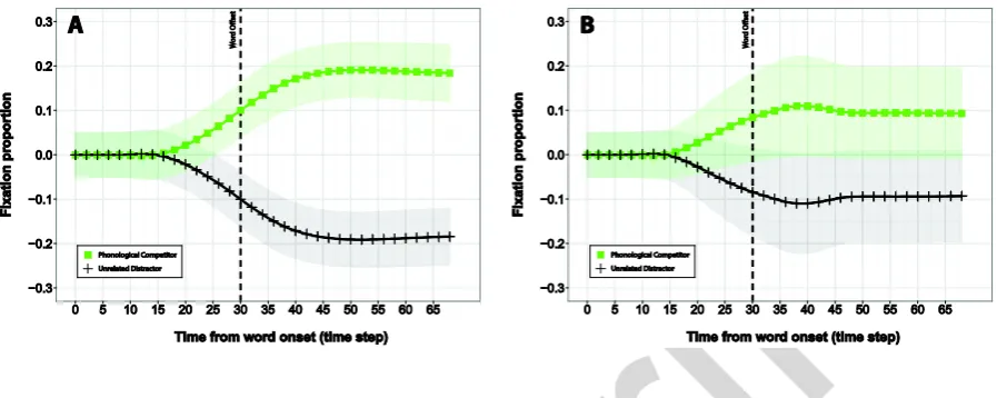
(34) Figure 5 displays the change from word onset in the probability of fixating each category of item. 2. (rhyme competitor, unrelated distractor) averaged over the 10 test trials for parameterisation 1. 3. (Figure 5A) and parameterisation 2 (Figure 5B) of the extended TRACE model.. 4. pr in. t. 1. Figure 5: Change from word onset in the probability of fixating rhyme competitors and unrelated. 6. distractors as predicted by the extended TRACE model. (A) behaviour generated by parameterisation. 7. 1, (B) behaviour generated by parameterisation 2. Shaded areas define 95% confidence intervals.. 8. We applied the same method of analysis as described in section 2.2 to the probabilities of fixating. 9. each category of object generated by the extended TRACE model. We first divided the 70 time step. 10. test trial into five time windows. A baseline time window was recorded as the period from trial onset. 11. to word onset (6 time steps: ts -6 to 0). The remainder of the trial, the period post word onset, was. 12. then divided into four equal length windows (ts 1 - 16; ts 17 - 32; ts 33 - 48; ts 49 - 64). For each window. 13. we calculated the empirical log odds of fixating each category of item. Our dependent measure was. 14. again the difference between the log odd of fixating the phonological rhyme competitor and the log. 15. odds of fixating the unrelated distractor. Using linear mixed effects models with a fixed effect of time. 16. window and a random effect of item (n = 10), including random intercepts for time window we. 17. examined whether our dependent measure differed in the baseline time window (ts -6 to 0) from that. 18. recorded in each of the time windows post word onset.. Pr. e-. 5. 33.

(35) This analysis revealed that fixation behaviour did not differ from baseline levels in the time period ts. 2. 1 -16 for either parameterisation of the model (parameterisation 1 (P1): β = -0.001, t = -0.26, p = 0.792;. 3. parameterisation 2 (P2): β = 0.0001, t = 0.03, p = 0.976). However, the rhyme competitor was fixated. 4. more than the unrelated distractor relative to baseline levels in time windows ts 17 - 32 (P1: β = 0.427,. 5. t = 15.11, p < 0.001; P2: β = 0.408, t = 3.65, p < 0.001), ts 33 - 58 (P1: β = 1.309, t = 28.58, p < 0.001;. 6. P2: β = 0.795, t = 3.98, p < 0.001) and ts 49 - 64 (P1: β = 1.490, t = 30.2, p < 0.001; P2: β = 0.723, t =. 7. 4.02, p < 0.001) for both parameterisations.. 8. 3.2.3. Summary. 9. The extended TRACE system fixates items that share their phonological rhyme with a spoken target. 10. word more than items that are unrelated in visual, semantic and phonological dimensions, thus. 11. replicating behaviour observed in previous visual world studies (Allopenna et al., 1998; Huettig &. 12. McQueen, 2012; McQueen & Viebahn, 2007). Both TRACE and the MIM predicted that effects emerge. 13. only post word offset. However, interpreting beta estimates as estimates of effect size indicates that. 14. the extended TRACE model predicted effects of phonological rhyme (P1: β = 1.490; P2: β = 0.723) at. 15. levels approximately twice the magnitude or greater than those predicted by the MIM (β = 0.486). 16. when rhyme competitors are presented alongside unrelated distractors.. 17. 3.3. Simulating effects of multimodal competition in TRACE. 18. In a second set of simulations we generate predictions using the extended TRACE system for how. 19. fixations would be distributed across scenes containing a rhyme competitor, a visual competitor, a. 20. semantic competitor and an unrelated distractor (conditions simulated in MIM in section 2.3).. 21. 3.3.1. Procedure. 22. Again ten trials were run with each parameterisation of the model. Each trial tested the model on a. 23. distinct set that included a rhyme competitor, visual competitor, semantic competitor and unrelated. Pr. e-. pr in. t. 1. 34.

No results found