©2018 The Authors Journal of the Royal Statistical Society: Series A (Statistics in Society) Published by John Wiley & Sons Ltd on behalf of the Royal Statistical Society.
This is an open access article under the terms of the Creative Commons Attribution-NonCommercial License, which permits use, distribution and reproduction in any medium, provided the original work is properly cited and is not used for commercial purposes.
0964–1998/19/182689
182,Part2,pp.689–711
Bayesian forecasting of mortality rates by using
latent Gaussian models
Angelos Alexopoulos,
University of Cambridge, UK
Petros Dellaportas
University College London, Alan Turing Institute, London, UK, and Athens University of Economics and Business, Greece
and Jonathan J. Forster
University of Southampton, UK
[Received October 2017. Revised October 2018]
Summary. We provide forecasts for mortality rates by using two different approaches. First we employ dynamic non-linear logistic models based on the Heligman–Pollard formula. Second, we assume that the dynamics of the mortality rates can be modelled through a Gaussian Markov random field. We use efficient Bayesian methods to estimate the parameters and the latent states of the models proposed. Both methodologies are tested with past data and are used to forecast mortality rates both for large (UK and Wales) and small (New Zealand) populations up to 21 years ahead. We demonstrate that predictions for individual survivor functions and other posterior summaries of demographic and actuarial interest are readily obtained. Our results are compared with other competing forecasting methods.
Keywords: Actuarial science; Demography; Heligman–Pollard model; Markov random field
1. Introduction
1.1. Problem setting
Analysis of mortality data has long been of interest to actuaries, demographers and statisticians. The first life tables were developed in the 17th century; see for example Graunt (1977). What is perhaps the best-known mortality function is the analytical formula that was suggested by Benjamin Gompertz in 1825 (Smith and Keyfitz, 1977), which in many cases gives surprisingly good fits to empirical adult mortality rates. The earliest attempt to represent mortality at all ages is that of Thiele and Sprague (1871), who combined three different functions to represent death rates among children, young to middle-aged adults and the elderly. They proposed negative and positive exponential curves for the first and third components and a normal curve for the second. Over a century later, Heligman and Pollard (1980) used a similar mathematical function that appears to provide satisfactory representations of a wide variety of mortality patterns across the entire age range.
Address for correspondence: Angelos Alexopoulos, Medical Research Council Biostatistics Unit, Cambridge Institute of Public Health, Forvie Site, Robinson Way, Cambridge Biomedical Campus, Cambridge, CB2 0SR, UK.
Demographers, economists and social scientists are interested not only in the actual demo-graphic structure of a country, but also on projections into the future. Although the static problem is quite straightforward, obtained readily from consensus data, the dynamic problem is a challenging problem with only partially satisfactory solutions. A wide variety of mortality projection models are now available for practitioners; see for example Lee and Carter (1992), Brouhnset al.(2002), Currieet al.(2004), Renshaw and Haberman (2006), Cairnset al.(2006) and Delwardeet al.(2007). The approach that has been adopted until now is to select a single model, based on considerations of goodness of fit, past practice or other considerations, and to project forwards in time to produce not only expected future mortality rates but also an estimate of the associated uncertainty in the form of a prediction interval. For a visual illustration of the problem consider the mortality data of UK–Wales, obtained from the Human Mortality Database (2014), between the years 1960 and 2013 depicted in Fig. 1. Clearly the probabilities of death are decreasing over the years and it is of particular interest to predict future mortality curves.
In what follows,mzt is used to represent the average, over timet, of the instantaneous rate of death among the individuals with age in the interval [z,z+1/; withnzt anddzt we denote the population at risk and the number of people who die at time t with age in the interval [z,z+1/, and following Currie (2016) we define the mortality ratepztto be the probability of dying within 1 year for a person agedzat timet. The density of au-variate Gaussian random variableX=.X1,: : :,Xu/with meanμand covariance matrixSevaluated atXis denoted by
φu.X;μ,S/. Furthermoreφu.X;μ,S,η,ξ/, whereη=.η1,: : :,ηu/andξ=.ξ1,: : :,ξu/, denotes the density ofXconditionally on the event thatXi∈[ηi,ξi],i=1,: : :,u, andηiandξiare either real numbers, or −∞or ∞ respectively; Nu.μ,S;η,ξ/denotes the corresponding u-variate truncated Gaussian distribution. By assuming that we have past data containing the number of people being at risk at timetagedzand the corresponding number of deathsdzt, our interest lies in forecasting the valuespz.T+1/,pz.T+2/,: : :.
1.2. A review of modelling and forecasting mortality rates
Useful review material and case-studies comparing models are provided by Booth and Tickle (2008), Cairnset al.(2011a) and Haberman and Renshaw (2011). Here we categorize mortality models into three main types.
1.2.1. Lee–Carter model and extensions
The best-known mortality model, and most successful in terms of generating extensions, is the Lee–Carter (LC) model (Lee and Carter, 1992) which models the logarithm ofmztas a bilinear function of age and time, i.e.
log.mzt/=az+βzζt .1/
where az,βz andζt are parameters to be estimated from relevant data. A time series model is used for ζt, which allows projections to be made by using estimates of futureζt based on the corresponding time series forecast. Renshaw and Haberman (2003) added flexibility to the model by incorporating a second bilinear term on the right-hand side of equation (1).
−10.0
−7.5
−5.0
−2.5
02
5
5
0
7
5
Age
Probability of death (log−scale)
Fig.
1.
F
rom
top
to
bottom,
log-probabilities
of
death
v
ersus
age
,
for
the
y
ears
1960,
1970,
1980,
1990,
2000,
2010
and
2013
fo
r
females
from
UK–W
Various extensions of the basic LC model have been proposed, most notably the introduction of cohort effects (Renshaw and Haberman, 2006), where model (1) is modified to
log.mzt/=az+βz.0/γt−z+βz.1/ζt .2/
whereβ.z0/γt−zrepresents a bilinear effect depending on cohortt−z.
The basic LC model does not impose any smoothness on the age parametersazandβz, which particularly in the case of βz can result in estimates which are unrealistic as functions of z. Approaches to overcome this problem involve smoothing the age parameters, either explicitly by constructing a smooth parametric model (de Jong and Tickle, 2006) or by imposinga priori
smoothing constraints on the parameters either via penalized maximum likelihood estimation (Delwardeet al., 2007) or, in a Bayesian framework, via a hierarchical prior distribution (Girosi and King, 2008). A related approach that was proposed by Hyndman and Ullah (2007) smooths the observed log.mzt/data by using standard non-parametric smoothing techniques and then fits a functional regression model to the smoothed data by using a set of orthonormal basis functions of age. The corresponding functional regression coefficients are time varying and projected by using a time series model. Recently, Liet al.(2013) proposed also some extensions to the basic LC model. First, following Li and Lee (2005), they modified the LC method to produce projections that are non-divergent between the two sexes. Then, they extended the model to account for changes in the age-specific rates of mortality decline over the years. They model the fact that mortality decline is decelerating at younger ages and accelerating at old ages (Bongaarts, 2005) by modellingβzto depend on timetthrough suitable functions. They noted that their model is particularly useful for projections over very long time horizons, whereas it reduces to the LC method for less than 80-years-ahead predictions.
1.2.2. Generalized linear models
Several approaches have been proposed in which the bilinear term in model (2) is replaced by linear terms, the simplest of these being the classical age–period–cohort (APC) model
log.mzt/=az+βt+γt−z .3/
which is commonly used in demographic and epidemiological applications.
Renshaw and Haberman (2003) proposed (variations of) a model which can be expressed as
log.mzt/=az+βzt+γt
where theγtare used in modelling observed data, but implicitly set to 0 for future projections. Cairnset al.(2006) proposed the logistic–linear model
log
pzt 1−pzt
=ζ.1/
t +ζt.2/.z− ¯z/ .4/
1.2.3. Non-linear models
Various models have been proposed where mortality is expressed as a parametric function of age. Perhaps the best known of these is the Heligman–Pollard model (Heligman and Pollard, 1980) where the odds of death as a function of age are
pz 1−pz
=A.z+B/C+Dexp [−E{log.z/−log.F/}2]+GHz .5/
whereA,B,C,D,E,F,GandH are unknown parameters. ParametersA,B,CandDtake values in the interval.0, 1/, whereas for the parametersE andF we have thatE∈.0,∞/and F∈.10, 40/. Finally,G∈.0, 1/andH∈.0,∞/; see Dellaportaset al.(2001) for a more detailed discussion. Rogers (1986) and Congdon (1993) have noted that estimation of the parameters of the Heligman–Pollard model is problematic because of the overparameterization of the model. Dellaportaset al.(2001) discussed the use of weighted least squares for the estimation of the Heligman–Pollard model and suggested Bayesian inference through a Markov chain Monte Carlo (MCMC) algorithm. Forecasting the future is more involved. The approach that has been adopted until now is first to estimate the parameters of the model for each age and for each year interval and then to model the estimated parameters via a time series model. Clearly, such approaches ignore the parameter uncertainty as well as the parameter dependence. These approaches have been adopted by Forfar and Smith (1985), Rogers (1986), McNown and Rogers (1989), Thompsonet al.(1989) and Denuit and Frostig (2009).
Sherris and Njenga (2011) described an approach to mortality forecasting by fitting a Heligman–Pollard model to the probabilities of death pzt, over time, with time varying pa-rametersAt,Bt,Ct,Dt,Et,Ft,Gt andHt. A vector auto-regression was used to model and project these time varying estimated parameters to obtain mortality projections.
1.3. Our contribution
We propose two modelling approaches to perform our predictions. First we generalize the work of Dellaportaset al.(2001) by including a dynamic component in their model based on the Heligman–Pollard formula. We assume that the eight parameters of the model evolve as random-walk parameters, thus relaxing any stationarity assumptions for the characteristics of the mortality curve. Second, we propose the use of a non-isotropic Gaussian Markov random field (GMRF) on a lattice constructed with ages zand years tand we project to the future by exploiting the estimated past features of the process. For both of the models proposed we use Bayesian methods to estimate their latent states and their parameters. More precisely, both models belong to the class of latent Gaussian models. The models consist of a non-normal likelihood and a Gaussian prior for their latent states. Bayesian inference for this type of models relies on an MCMC algorithm which alternates sampling from the full conditional distributions of the parameters of the model and the vector of the latent states.
discretization of the Langevin diffusion and they are used in the Metropolis adjusted Langevin algorithm that was developed by Roberts and Tweedie (1996) and the manifold Metropo-lis adjusted Langevin algorithm and Riemann manifold Hamiltonian Monte Carlo method developed by Girolami and Calderhead (2011). Proposals that take into account the depen-dence structure of the Gaussian prior of the latent states have been designed by Neal (1998) and by Murray and Adams (2010); see also Beskoset al.(2008) for a detailed discussion. Finally, Cotteret al.(2013) and Titsias and Papaspiliopoulos (2018) constructed proposal distributions which are informed from both the likelihood and the prior. In this paper we construct proposals that exhibit these properties in both of the models proposed.
1.4. Structure of the paper
The paper is organized as follows. In Section 2 we present our model based on the Heligman– Pollard formula. In Section 3 we adopt our second approach in the problem where we use a non-parametric model based on Gaussian processes. In Section 4 we present the application of our models on the UK–Wales and New Zealand data and we compare them with other competing models. Section 5 concludes with a brief discussion.
The data that are analysed in the paper and the programs that were used to analyse them can be obtained from
https://rss.onlinelibrary.wiley.com/hub/journal/1467985x/series-a-datasets
2. A dynamic model based on Heligman–Pollard formula
Heligman and Pollard (1980) argued that a mortality graduation can only be considered suc-cessful if the graduated rates progress smoothly from age to age and at the same time they reflect accurately the underlying mortality pattern. For this reason they proposed a mathematical ex-pression or law of mortality which they fitted to post-war Australian national mortality data.
The curve that they suggested is given by equation (5). To define the dynamic version of the model, letψt=.A˜t,B˜t,C˜t,D˜t,E˜t,F˜t,G˜t,H˜t/be the latent states of the model parameters at timet, where the elements ofψt are obtained from the original variables by using a suitable transformation so thatψt∈R8. For example we setA˜t=log{At=.1−At/} andE˜t=log.Et/. Throughout this paper,t will refer to a year whereas T is the number of years in the past for which we have data. The odds of death at time point t are assumed to be given by the Heligman–Pollard model:
pzt 1−pzt
=A.zt +Bt/Ct+Dtexp [−Et{log.z/−log.Ft/}2]+GtHtz .6/
wherez=0, 1,: : :,ω,t=1,: : :,Tandωis the age of the oldest people in the data. We denote the right-hand side of equation (6) byK.z,ψt/and we have that
pzt= K.z
,ψt/
1+K.z,ψt/ .7/
whereas the likelihood of our model is
π.d|ψ/=T
t=1
ω
z=0
nzt dzt
K.z,ψt/dzt{1+K.z,ψt/}−nzt .8/
For the dynamic modelling of the latent states inψtwe assume a random-walk structure and we have that
π.ψt|ψt−1,μ,Σ,η,ξ/=φ8.ψt;ψt−1+μ,Σ,η,ξ/, t=2,: : :,T, .9/ π.ψi1/∝1 ifψi1∈[ηi,ξi] andπ.ψi1/=0 otherwise, whereψit denotes the ith element of ψt, i=1,: : :, 8.
The random-walk process that is defined by equation (9) imposes a large amount of prior structure for the parameters of the Heligman–Pollard model and relaxes any stationarity as-sumptions for their evolution across the years. Specification of the vectors η and ξ allows the representation of our prior beliefs about the range of the parameters of the model and restricts known problems such as overparameterization (Congdon, 1993), non-identifiability (Bhatta and Nandram, 2013) and change in age patterns of mortality decline (Liet al., 2013) across the years. In our applications we fix the elements of the vectorsη andξon the basis of prior beliefs, expressed as 1% and 99% percentiles, reported by Dellaportaset al.(2001), by settingη=.−10:61,−10:61,−5:99,−11:29,−25:33,− ∞,−17:5,−1:39/andξ=.−2:75,
−0:2, 2:2,−3:48, 4:09, 2:64,−3:48, 0:18/.
For the driftμof the random-walk process we assume thatπ.μ/=φ8.μ; 0,M−1/, whereM is a diagonal 8×8 matrix with elements equal to 0.001. For the variance–covariance matrixΣ we assume the following inverse Wishart prior that was suggested by Huang and Wand (2013):
Σ|α∼IW.ν+8−1, 2νΣprior/
whereα=.α1,: : :,α8/,Σprioris a diagonal matrix with elements 1=α1,: : :, 1=α8on the diagonal,
ν+8−1 are the degrees of freedom of the inverse Wishart distribution and for the parameters
αiwe assume the following inverse gamma prior distributions:
αi
IID
∼IG.12, 1=l2/
for alli=1,: : :, 8 whereas, following Huang and Wand (2013), we setl=105. This prior structure implies half-t.ν,l/prior distributions for the standard deviationsσi in the diagonal ofΣand by choosingν=2 we have uniformU.−1, 1/prior distributions for the correlation of the latent states inψt; see Gelman (2006) and Huang and Wand (2013) for a detailed presentation of this prior distribution for the covariance matrix Σ. Denoting byθ=.Σ,μ,α/the parameters of the model and byψ=.ψ1,: : :,ψT/the latent states of the model the posterior distribution of interest is
π.ψ,θ|d,η,ξ/∝π.θ/π.d|ψ/T
t=2
φ8.ψt;ψt−1+μ,Σ,η,ξ/: .10/
By noting that any of the conditional distributions for the elements ofψdepend on the vectors η and ξ, we simplify our notation and we drop reference to them for the remainder of the section.
Our aim is to predict the probabilitiespztat some future time pointst=T+1,T +2,: : :, for allz=0, 1,: : :,ω. To compute, for example, the posterior predictive distribution ofpz,T+1, we
first must approximate
π.ψT+1|d/=
π.ψT+1|ψT,θ/π.ψ,θ|d/dψdθ .11/
and then compute the predictive density ofpz,T+1based on equation (7). The integral in equation
samples from the distribution with densityπ.ψ,θ|d/and then for each sampleψmandθmwe draw ψm
T+1from the distribution with densityφ8.ψT+1;ψmT +μm,Σm,η,ξ/. The values{ψmT+1}Mm=1
form, through equation (7), a sample from the posterior predictive distribution ofpz,T+1. The
same procedure can be used for every future time pointT+2,T+3,: : :.
It is clear from expression (10) that the model proposed is a latent Gaussian model with latent statesψand hyperparametersθ. To obtain samples from distribution (10) we construct a Metropolis-within-Gibbs sampler which alternates sampling fromπ.ψ|θ,d/andπ.θ|ψ,d/. Sampling fromπ.θ|ψ,d/can be conducted directly since the full conditional distributions of the hyperparametersΣ,μandαare of known form. Sampling fromπ.ψ|θ,d/is performed by usingT MH steps to update eachψt. In Section 5 of the on-line supplementary material we derive the full conditional distributions required.
An important feature of the MH steps that we use to sample from the distribution with densityπ.ψ|θ,d/is as follows. We incorporate information from the likelihood of our model in the proposal distributions of the MH steps by following Dellaportaset al.(2001). We pro-pose for each t=1,: : :,T new states for ψt from a Gaussian distribution with meanmt and covariance matrixctVt. The vectormt and the covariance matrixVt are the maximum likeli-hood estimators and covariance (inverse Hessian) matrix derived by using a non-linear weighted least squares algorithm with weightswzt=1=qzt2, whereqztare the empirical mortality rates, for the age zat time pointt, as suggested by Heligman and Pollard (1980). Finally,ct are pre-specified constants, which are tuned to achieve better convergence behaviour measured with respect to sampling efficiency (the percentage of accepted proposed moves). After the initial iteration, the mean vector of the proposal density is updated with the current sampled parame-ter vector. Thus, we construct a likelihood-informed proposal distribution which enables us to update the eight parameters of the model jointly. These characteristics of the proposed MCMC algorithm accelerate the convergence of the corresponding Markov chain by overcoming prob-lems such as the strong posterior correlation of the parameters of the Heligman–Pollard model that was reported by Dellaportaset al.(2001). In Section 4 we apply the present methodology to the UK–Wales and New Zealand data. We evaluate the mixing properties of the proposed MCMC algorithm using the effective sample size (ESS) of the samples drawn from the poste-rior distributions of interest. The ESS of M samples drawn by using an MCMC algorithm can be estimated as s2M=γ0 where s2 is the sample variance of the samples and γ0 is an estimate of the spectral density of the Markov chain at zero. In the on-line supplementary material we compare the ESS of samples drawn from the posterior in expression (10) by using our proposed MH steps with the ESS of samples drawn using simple random-walk MH steps.
3. A non-parametric model
A Markov random field is a joint distribution for the variables.x1,: : :,xn/which is determined by
its full conditional distributions with densitiesπ.xi|x−i/wherex−i=.x1,: : :,xi−1,xi+1,: : :,xn/.
In the case where the conditional distributions are Gaussian distributions the Markov random field is called a GMRF; see Rue and Held (2005). There is a strong connection between GMRFs and conditional auto-regressive models (Besag, 1974).
3.1. Modelling mortality rates by using an intrinsic Gaussian Markov random-field model
To model mortality rates based on the model with likelihood given by equation (8) we transform the probabilitypzt of death at agezin thetth year in the variablexzt=log{pzt=.1−pzt/}for eachz=0,: : :,ω andt=1,: : :,T:Denote byxt=.x0t,: : :,xωt/and letx=.x1,: : :,xT/be an .ω+1/T-dimensional vector. It is useful to think of a lattice with.ω+1/×T nodes and.z,t/ denoting the element of thezth row and thetth column. For the vectorxwe assume that it has an.ω+1/T-variate Gaussian distribution with meanμ=.b1ω+1, 2b1ω+1,: : :,Tb1ω+1/, where
1ω+1is an.ω+1/-dimensional vector with 1s, and precision matrix
Q=τ.ρageRω+1⊗IT+ρyearIω+1⊗RT/ .12/
whereIω+1is the identity matrix of dimension.ω+1/×.ω+1/andRω+1is an.ω+1/×.ω+1/
matrix with elementsRij defined as
Rij=
⎧ ⎪ ⎪ ⎪ ⎨ ⎪ ⎪ ⎪ ⎩
1 ifi=1 andj=1,
1 ifi=ω+1 andj=ω+1,
2 ifi=jandi,j=1 andi,j=ω+1,
−1 if|i−j| =1,
0 otherwise:
Following the modelling perspective describedxis an intrinsic GMRF sinceQis singular. It follows that, for eachz=1,: : :,ω−1 andt=2,: : :,T−1, the full conditional density ofxzt is normal with mean equal to
1
4{ρage.xz−1,t+xz+1,t/+ρyear.xz,t−1+xz,t+1/}
and variance 1=.4τ/. The parametersρageandρyearcontrol the association of the probabilities of death across ages and years respectively. We emphasize thatρage andρyearare expected to differ because they capture correlations across age and calendar time dimensions, whereas to guarantee model identifiability we assume thatρage+ρyear=2.
3.1.1. Bayesian inference
The likelihood function of our model is given by the product of the terms on the right-hand side of equation (8):
π.d|x/=T
t=1
ω
z=0
nzt dzt
pdztzt .1−pzt/nzt−dzt, .13/
wheredis the.ω+1/T-dimensional vector with elementsdztandpzt=exp.xzt/={1+exp.xzt/}. By denoting byθ=.b,ρage,τ/the parameters of the model, we construct an MCMC algorithm that samples from the joint posterior distribution of the parameters and the latent states of the model which has density
π.θ,x|d/∝π.θ/π.x|θ/π.d|x/,
whereπ.θ/is the density of the prior distribution of the parameters,π.x|θ/is the density of the (improper).ω+1/T-variate Gaussian distribution with meanμand precision matrixQand
π.d|x/is given by equation (13).
we note that we can sample from these either directly.τ,b/or by random-walk MH steps on
ρage.
Sampling fromπ.x|θ,d/consists of sampling from a distribution with density proportional to the product of the.ω+1/T-variate Gaussian prior of the latent statesxwith the intractable likelihood given by equation (13). We use the gradient-based auxiliary MCMC sampler that was proposed by Titsias and Papaspiliopoulos (2018) for sampling the latent states of the model proposed. In this case the gradient-based auxiliary sampler makes efficient use of the gradient information of the (intractable) likelihood and is invariant under the tractable Gaussian prior. Titsias and Papaspiliopoulos (2018) show, by conducting extensive experiments in the context of latent Gaussian models, that the gradient-based auxiliary sampler outperforms, in terms of the ESS, well-established methods such as the Metropolis adjusted Langevin algorithm (Roberts and Stramer, 2002), elliptical slice sampling (Murray and Adams, 2010) and preconditioned Crank-Nicolson Langevin algorithms (Cotteret al., 2013). Finally, an attractive feature of the gradient-based auxiliary sampler is that its implementation is straightforward and requires only a single tuning parameter to be specified, which can be estimated during the burn-in period.
The proposal that was developed by Titsias and Papaspiliopoulos (2018) is based on an idea that first appeared in Titsias (2011) and is constructed as follows. Auxiliary variablesux∈R.ω+1/T are drawn from the Gaussian distribution
N[x+.δ=2/∇log{π.d|x,θ/},.δ=2/I.ω+1/T]
where∇logπ.d|x,θ/denotes the gradient of the log-likelihood evaluated at the current states ofxandθ. Then new valuesxpropare proposed from the distribution with density
q.xprop|ux/∝φ.ω+1/T{xprop;ux,.δ=2/I.ω+1/T}π.xprop|θ/, .14/
and the proposed valuexpropis accepted with MH acceptance probability min.1,α/given by
α=π.πd|xprop,θ/
.d|x,θ/ exp{f.ux,xprop/−f.ux,x/} .15/
and f.ux,x/=.ux−x−.δ=4/∇log{π.d|x,θ/}/∇log{π.d|x,θ/}, whereas Titsias (2011) sug-gested tuning the parameterδfor an acceptance rate of 50–60% to be achieved. In section 2 of the on-line supplementary material we summarize the steps of this algorithm.
For everyzandk, our aim is to predict the probabilities of deathpzt at future time points t=T+1,T+2,: : :,T+kexpressed through the vectorsxÅ=.xT+1,: : :,xT+k/. The required predictive density is
π.xÅ|d/=
π.xÅ|x,θ/π.x,θ|d/dx dθ: .16/
In section 3 of the on-line supplementary material of the paper we describe how we approxi-mate the integral in equation (16) based on MCMC samples from the distribution with density
4. Applications to real data
4.1. Prediction of mortality rates
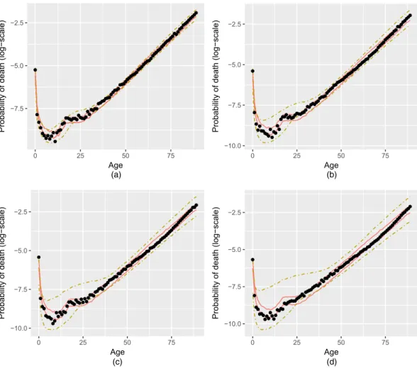
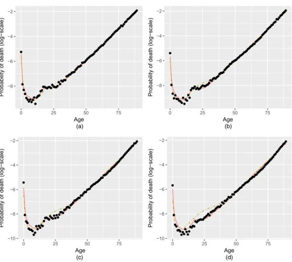
Our suggested models express different modelling beliefs about the extrapolation of the mortality curve. The Heligman–Pollard dynamic model suggests non-stationarity with variance increas-ing as the predictions move away in future, whereas the GMRF predictions are constrained by the strong Gaussian prior. To test how both models behave in real data, we predict 5-, 10-, 15-and 21-years-ahead mortality rates for UK–Wales based on observed data from the Human Mortality Database (2014) during years 1983–1992.T=10;ω=89/. The results are compared with true observed mortality rates. Fig. 2 depicts the 95% credible intervals of the posterior pre-dictive distributions of the log-probabilities of death obtained from the Heligman–Pollard and the non-parametric models, whereas Fig. 3 presents the corresponding posterior means. Both models perform well, with the Heligman–Pollard model achieving, as expected, wider credible intervals which are evaluated in Section 4.3 through a fully fledged quantitative evaluation. The methods proposed are not computationally expensive; our MCMC algorithms are written in R (R Core Team, 2017) and we obtain 1000 iterations in 2.5 min in the case of the GMRF model and in 6.5 s in the case of the Heligman–Pollard model. Thus, we needed almost 8 h to complete 21-years-ahead predictions by using the GMRF model and less than 4 h for the dynamic Heligman–Pollard model. However, after fitting the two models in multiple data sets in Section 4.3, we noted that the time for the Heligman–Pollard model varies between 4 and 14 h depending on the data set. See also the on-line supplementary material where we provide details for the implementation of our algorithm.
4.2. Prediction of survival probabilities
An attractive feature of our Bayesian methods is that we can easily obtain prediction intervals for several quantities which are of interest to actuaries and demographers, but they are not readily available in non-Bayesian models. Here we present projections of survival probabilities in a horizon ofkyears ahead. These are defined as
spz,T+k=
s−1
i=0
.1−pz+i,T+k/ .17/
and denote the probability of a person aged z at the yearT+k to survive up to age z+s. Following Dellaportaset al.(2001) we utilize samples from the posterior predictive distributions of the probabilities of death to compute the probabilities in equation (17) for the data that were presented in Section 4.1. Fig. 4 summarizes the posterior samples of survival probabilities for s=5, projected in the years 1997, 2002, 2007 and 2013 (k=5, 10, 15, 21) by using the GMRF model. It is clear that we predict an increase in the posterior survivor function (lifetime).
Finally, we note that forecasts for quantities such as life expectancies, median lifetime, joint (for two people) lifetime and the probability of the first who dies between two people could be obtained easily from the output of the MCMC algorithms proposed as well.
4.3. Comparisons with existing methods
We compare our forecasts of future mortality rates with forecasts that were obtained with a series of popular models available in the R package StMoMo (Villegas et al., 2018). The
StMoMopackage provides a set of functions for defining and fitting an abstract model from
●
● ● ●
●●●● ●●
● ● ●●●
●●●●●●●●● ●●●●●●●●●●●
●●●●●● ●●●
●●● ●●●●●
●●●●● ●●●●
●●●● ●●●●
●●●● ●●●●
●●●●● ●●●●
●●●●
−7.5 −5.0 −2.5
0 25 50 75
Age
Probability of death (log−scale)
●
● ●
●●●●●● ● ● ●●●
● ●
●●●●●●●●●●●●● ●●●●●
●●●● ●●●●●●
●●●● ●●●●●
●●●● ●●●●●
●●●● ●●●●
●●● ●●●●
●●●● ●●●●
●●●● ●
−10.0 −7.5 −5.0 −2.5
0 25 50 75
Age
Probability of death (log−scale)
●
● ●●
●●●● ●●
● ●●●●●
●●●●●●●●●● ●●●●●●
●●●●● ●●●●
●●●● ●●●●●
●●●●● ●●●●●
●●● ●●●●●●
●●●● ●●●●
●●●● ●●●●
●●●●●
−10.0 −7.5 −5.0 −2.5
0 25 50 75
Age
Probability of death (log−scale)
●
● ●●
●●● ●●●
● ●●●●●●●
●●●●●●●● ●●●●
●●●●●●●● ●●●●
●●●●● ●●●●●
●●●●● ●●●●●
●●●●● ●●●●●
●●●● ●●●●
●●●● ●●●●
●●
−10.0 −7.5 −5.0 −2.5
0 25 50 75
Age
Probability of death (log−scale)
(a) (b)
(c) (d)
Fig. 2. Predicted 95% credible intervals for the GMRF ( ) and the Heligman–Pollard ( ) models
for UK–Wales mortality data based on observations for the years 1983–1992 (
, true log-probabilities ofdeath): (a) predictions for 1997; (b) predictions for 2002; (c) predictions for 2007; (d) predictions for 2013
projections arising from the estimation of the parameters of a model, the package provides also functions for the implementation of bootstrap (semiparametric or on residuals) techniques as was suggested by Brouhnset al.(2005), Koissiet al.(2006) and Renshaw and Haberman (2008). Here, we compare predictions for mortality rates obtained by using our Bayesian methods with predictions obtained by using three commonly used stochastic mortality models. These are the LC model (Lee and Carter, 1992) presented by equation (1), the APC model defined by equation (3) and the model of Plat (2009) which combines the model of Cairnset al.(2006) presented by equation (4) with some features of the LC model.
●
● ●
● ●●●●●●●
● ●●●
●●●●●●●●● ●●●●●●●●●●●
●●●●● ●●●●
●●● ●●●●●
●●●● ●●●
●●●●● ●●●
●●●● ●●●●
●●●●● ●●●●
●●●● ●●
−8 −6 −4 −2
0 25 50 75
Age
Probability of death (log−scale)
●
●
● ●●●●●●
● ●
●●● ● ●
●●●●●●●●●●●●● ●●●●●
●●●● ●●●●
●●●● ●●●●●
●●●● ●●●●●
●●●● ●●●●
●●● ●●●●
●●●● ●●●
●●●●● ●●●
−8 −6 −4 −2
0 25 50 75
Age
Probability of death (log−scale)
●
● ●●
●●●● ●●
● ●●●●●
●●●●●●●●●● ●●●●●●
●●●●● ●●●
●●●●● ●●●●●
●●●●● ●●●●●
●●● ●●●●●
●●●● ●●●●
●●●● ●●●●
●●● ●●●
−10 −8 −6 −4 −2
0 25 50 75
Age
Probability of death (log−scale)
●
●
●● ●●●
●●● ● ●
●● ●●●●
●●●●●●●● ●●●●
●●●●● ●●●●
●●●●● ●●●●●
●●●●● ●●●●
●●●●● ●●●●
●●●● ●●●●
●●●● ●●●●
●●● ●●●●
−10 −8 −6 −4 −2
0 25 50 75
Age
Probability of death (log−scale)
(a) (b)
(c) (d)
Fig. 3. Predicted means for the GMRF ( ) and the Heligman–Pollard ( ) models for UK–Wales
mortality data based on observations for the years 1983–1992 (, true log-probabilities of death): (a)
predic-tions for 1997; (b) predicpredic-tions for 2002; (c) predicpredic-tions for 2007; (d) predicpredic-tions for 2013
●●●●●●● ●●●●●●●●●●●●●● ●●●● ●●●●●● ●●● ●●●●●●● ●●●●●●●●●●●●● ●●●●●●● ●●●●●●●●●● ●●●●●● ●● ●●●●●● ●●●●●● ●● ● ●● ● ●● ● ●● ●●● ● ●●●● ●●● ● ● ● ●● ●● ●●●● 0.5 0.6 0.7 0.8 0.9 1.0 0 5 10 15 20 25 30 35 40 45 50 55 60 65 70 75 80 85 Age Probability ● ●●●●●●● ●●●●●●● ●●●●●● ●●●●●●●● ●●●●●●●● ●●●●●●● ●●●●●●●●●●●●●●●●●●●●● ●●●●●●●● ●●●●●●●● ●●●●● ● ●●●●● ● ●●●●●● ●●●●●●●● ● ●● ●●● ● ●● ● ● ● ●● ● ● ● ●●●● ● ● ● ● ● ●● ● ●●● ● ● 0.5 0.6 0.7 0.8 0.9 1.0 0 5 10 15 20 25 30 35 40 45 50 55 60 65 70 75 80 85 Age Probability ●●●●●●●●● ●●●●●●●●●●●● ●●●●●● ●●● ●●●●● ●●●●●●●●●●●● ●●●●●●●●● ●●●●●●●●●● ●●●● ●●●●●●● ●●●●●●●●●●● ●●●●●●●●●● ●● ● ●● ●● ●● ●● ●● ●●●●● ●● ●●●●● ●● ●● ●●● ● ●● ●● ● ●●● ● ● ● ● ● ● ● ●● ●●● ● ●●● ● ● ● ● ● 0.5 0.6 0.7 0.8 0.9 1.0 0 5 10 15 20 25 30 35 40 45 50 55 60 65 70 75 80 85 Age Probability ●●●●●●●●●●●● ●●●●●●●● ●●●●●●●●●● ●●●●●●● ●●●●●●●●●●●● ●●●●●●●●●●● ●●●●●●●●●●●●●●●● ●●●●●●●●●●●● ●●●●●●●●● ● ●●●●●●●●●●●●●● ● ●●●●●● ●●● ●●●●●● ● ●● ● ● ● ●●●● ● ● ●● ●●●●●●● ● ● ●●●●● ●● ● ●● ●●● ● ● ● 0.5 0.6 0.7 0.8 0.9 1.0 0 5 10 15 20 25 30 35 40 45 50 55 60 65 70 75 80 85 Age Probability ( a )( b ) (c) (d) Fig. 4. P oster ior predictiv e distr ib utions of sur viv al probabilities s
pz,
To assess the quality of the prediction intervals obtained for the future probabilities of death we calculated the empirical coverage probabilities of the prediction intervals obtained, the mean width of the prediction intervals and the mean interval score. The quality of the mean forecasts was assessed by using the root-mean-squared error of the predicted means. For a fixed prediction horizonkand agezthe empirical coverage probability of the prediction interval obtained from a given model was computed as the proportion of the 25−kintervals that include the observed probability of death at agezat the yearT+k, forT=1989,: : :, 2013−k. The mean width of the prediction interval is the sample mean of the 25−kwidths of the prediction intervals obtained and the mean interval score is the sample mean of the scoring rule called the interval score; see equation (43) in Gneiting and Raftery (2007). As was explained in Gneiting and Raftery (2007) the interval score is a scoring rule which rewards the forecaster who obtains narrow prediction intervals and incurs a penalty, proportional to the level of significance of the interval, if the observation misses the prediction interval. This means that we would like to obtain prediction intervals with low mean interval score. See also the on-line supplementary material of the present paper for a more detailed presentation of the interval score.
Figs 5 and 6 visualize the evaluation of the 95% prediction intervals that were obtained from the models under comparison for the UK–Wales data set. It seems that for the majority of the ages in the range 10–50 years old the proposed non-isotropic GMRF model delivers the most satisfactory predictions, for prediction horizons of both 5 and 15 years ahead, whereas for ages after 60 years the APC and Plat (2009) models exhibit slightly better predictive performance. Figs 7 and 8 depict the evaluation of the predictions that were obtained by the models under comparison for the mortality data from New Zealand. For a horizon of 5 years ahead the predictions of the Heligman–Pollard model are more accurate than those obtained from the LC, the APC and the Plat (2009) models for most of the ages up to 60 years old, whereas for predictions of 15 years ahead the APC and Plat (2009) models exhibit the best predictive performance for almost the whole age range.
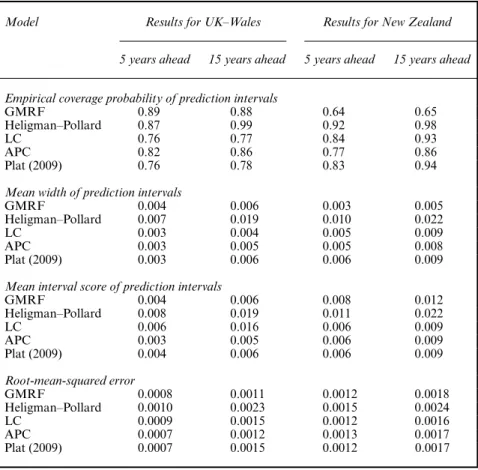
In Table 1 we summarize the results that are presented in Figs 5–8 by providing averages, over ages, of the four measures that we used to assess the predictions that were obtained from the mod-els under comparison. The non-isotropic GMRF model proposed dominates the Heligman– Pollard model in all the measures that we used except that from the coverage probabilities in the case of the New Zealand data set. Nevertheless, even in this case the superiority of the Heligman–Pollard model is quite unimportant since it is based on very wide prediction inter-vals which have little practical importance. Moreover, Bayesian inference for the parameters of the dynamic Heligman–Pollard model requires a large amount of prior information whereas inference for the GMRF model is feasible with non-informative priors. In summary, we propose the use of the GMRF model except if one wishes to relax the stationarity assumptions of the evolution of the mortality curves over the years via the Heligman–Pollard model.
0.4 0.6 0.8 1.0 0 5 10 15 Age Cove rage probability 0.25 0.50 0.75 1.00 15 20 25 30 35 40 Age Cove rage probability 0.4 0.6 0.8 1.0 40 50 60 70 80 90 Age Cove rage probability 0.000 0.001 0.002 0.003 0 5 10 15 Age
Mean width of prediction interv al 1e−04 2e−04 3e−04 15 20 25 30 35 40 Age
Mean width of prediction interv al 0.00 0.02 0.04 0.06 40 50 60 70 80 90 Age
0.00 0.25 0.50 0.75 1.00 0 5 10 15 Age Cove rage probability 0.25 0.50 0.75 1.00 15 20 25 30 35 40 Age Cove rage probability 0.00 0.25 0.50 0.75 1.00 40 50 60 70 80 90 Age Cove rage probability 0.000 0.002 0.004 0.006 0 5 10 15 Age
Mean width of prediction interv al 0.00000 0.00025 0.00050 0.00075 0.00100 0.00125 15 20 25 30 35 40 Age
Mean width of prediction interv al 0.00 0.05 0.10 0.15 40 50 60 70 80 90 Age
0.4 0.6 0.8 1.0 0 5 10 15 Age Cove rage probability 0.4 0.6 0.8 1.0 15 20 25 30 35 40 Age Cove rage probability 0.4 0.6 0.8 1.0 40 50 60 70 80 90 Age Cove rage probability 0.000 0.005 0.010 0 5 10 15 Age
Mean width of prediction interv al 2e−04 3e−04 4e−04 5e−04 6e−04 7e−04 15 20 25 30 35 40 Age
Mean width of prediction interv al 0.000 0.025 0.050 0.075 0.100 40 50 60 70 80 90 Age
0.25 0.50 0.75 1.00 0 5 10 15 Age Cove rage probability 0.2 0.4 0.6 0.8 1.0 15 20 25 30 35 40 Age Cove rage probability 0.4 0.6 0.8 1.0 40 50 60 70 80 90 Age Cove rage probability 0.00 0.02 0.04 0.06 0 5 10 15 Age
Mean width of prediction interv al 0.001 0.002 0.003 15 20 25 30 35 40 Age
Mean width of prediction interv al 0.0 0.1 0.2 0.3 40 50 60 70 80 90 Age
Table 1. Predictive performance of various models: the average predictive measure over the ages 0–89 years is reported
Model Results for UK–Wales Results for New Zealand
5 years ahead 15 years ahead 5 years ahead 15 years ahead
Empirical coverage probability of prediction intervals
GMRF 0.89 0.88 0.64 0.65
Heligman–Pollard 0.87 0.99 0.92 0.98
LC 0.76 0.77 0.84 0.93
APC 0.82 0.86 0.77 0.86
Plat (2009) 0.76 0.78 0.83 0.94
Mean width of prediction intervals
GMRF 0.004 0.006 0.003 0.005
Heligman–Pollard 0.007 0.019 0.010 0.022
LC 0.003 0.004 0.005 0.009
APC 0.003 0.005 0.005 0.008
Plat (2009) 0.003 0.006 0.006 0.009
Mean interval score of prediction intervals
GMRF 0.004 0.006 0.008 0.012
Heligman–Pollard 0.008 0.019 0.011 0.022
LC 0.006 0.016 0.006 0.009
APC 0.003 0.005 0.006 0.009
Plat (2009) 0.004 0.006 0.006 0.009
Root-mean-squared error
GMRF 0.0008 0.0011 0.0012 0.0018
Heligman–Pollard 0.0010 0.0023 0.0015 0.0024
LC 0.0009 0.0015 0.0012 0.0016
APC 0.0007 0.0012 0.0013 0.0017
Plat (2009) 0.0007 0.0015 0.0012 0.0017
this paper may be a little tricky and may vary between our two proposed models, since their full conditional density depends not only on the aggregated mortality rates of that year but also on the possibly unobserved mortality rates at the same age of other years.
5. Conclusions
We have proposed two models for forecasting mortality rates. We have first taken up the theme in Dellaportaset al. (2001) that there are a few attempts at modelling the time evolution of the Heligman–Pollard formula and we proposed a model that does not respect stationarity in the dynamic modelling of the parameters. We have also proposed a non-parametric model based on non-isotropic GMRFs. The evaluation of the forecasts that were obtained from the proposed and from existing models provides evidence that there are advantages in predicting future mortality rates by using our Bayesian models.
16-dimensional density with the covariance matrixΣcapturing dependences of the parameters of the two populations. In the case of the GRMF model the dimension of eachxt could be a .2ω+2/-dimensional vector resulting in a.2ω+2/T×.2ω+2/T precision matrix in equation (12) which could be modelled by constructing a non-isotropic GMRF of higher order; see for example chapter 3 of Rue and Held (2005).
It is well known in the demographic literature (see for example Renshaw and Haberman (2008)) that it is quite important for demographers, insurance companies and pension institutes that the uncertainty of the projections of future mortality rates is quantified through the compu-tation of prediction intervals. Our proposed Bayesian methodology clearly addresses this issue by producing predictive densities of future data. This feature, together with the fact that one can produce any predictive quantities of interest with simple manipulations of our MCMC output, makes our predictions very valuable to actuaries and demographers alike.
Acknowledgements
We are grateful to the reviewers for valuable suggestions on presentation and modelling and to Michalis Titsias for many helpful discussions. This research has been cofinanced by the European Union (European Social Fund) and Greek national funds through the operational programme ‘Education and lifelong learning’ of the national strategic reference framework, research funding programme ARISTEIA-LIKEJUMPS-436, and by the Alan Turing Institute under Engineering and Physical Sciences Research Council grant EP/N510129/1.
References
Besag, J. (1974) Spatial interaction and the statistical analysis of lattice systems (with discussion).J. R. Statist. Soc.B,36, 192–236.
Beskos, A., Roberts, G., Stuart, A. and Voss, J. (2008) MCMC methods for diffusion bridges.Stoch. Dynam.,8, 319–350.
Bhatta, D. and Nandram, B. (2013) A bayesian adjustment of the HP law via a switching nonlinear regression model.J. Data Sci.,11, 85–108.
Bongaarts, J. (2005) Long-range trends in adult mortality: models and projection methods.Demography,42, 23–49.
Booth, H. and Tickle, L. (2008) Mortality modelling and forecasting: a review of methods.Ann. Act. Sci.,3, 3–43. Brouhns, N., Denuit, M. and Van Keilegom, I. (2005) Bootstrapping the Poisson log-bilinear model for mortality
forecasting.Scand. Act. J., no. 3, 212–224.
Brouhns, N., Denuit, M. and Vermunt, J. K. (2002) A Poisson log-bilinear regression approach to the construction of projected lifetables.Insur. Math. Econ.,31, 373–393.
Cairns, A. J., Blake, D. and Dowd, K. (2006) A two-factor model for stochastic mortality with parameter uncer-tainty: theory and calibration.J. Risk Insur.,73, 687–718.
Cairns, A. J., Blake, D., Dowd, K., Coughlan, G. D., Epstein, D. and Khalaf-Allah, M. (2011a) Mortality density forecasts: an analysis of six stochastic mortality models.Insur. Math. Econ.,48, 355–367.
Cairns, A. J., Blake, D., Dowd, K., Coughlan, G. D. and Khalaf-Allah, M. (2011b) Bayesian stochastic mortality modelling for two populations.Astin Bull.,41, 29–59.
Carter, C. K. and Kohn, R. (1994) On Gibbs sampling for state space models.Biometrika,81, 541–553. Congdon, P. (1993) Statistical graduation in local demographic analysis and projection.J. R. Statist. Soc.A,156,
237–270.
Cotter, S. L., Roberts, G. O., Stuart, A. M. and White, D. (2013) MCMC methods for functions: modifying old algorithms to make them faster.Statist. Sci.,28, 424–446.
Currie, I. D. (2016) On fitting generalized linear and non-linear models of mortality.Scand. Act. J., no. 4, 356–383.
Currie, I. D., Durban, M. and Eilers, P. H. (2004) Smoothing and forecasting mortality rates.Statist. Modllng,4, 279–298.
Dellaportas, P., Smith, A. F. and Stavropoulos, P. (2001) Bayesian analysis of mortality data.J. R. Statist. Soc.
A,164, 275–291.
Denuit, M. and Frostig, E. (2009) Life insurance mathematics with random life tables.Nth Am. Act. J.,13, 339–355. Forfar, D. and Smith, D. (1985) The changing shape of English life tables.Trans. Faclty Act.,40, 98–134. Gamerman, D. (1997) Sampling from the posterior distribution in generalized linear mixed models.Statist.
Comput.,7, 57–68.
Gamerman, D. (1998) Markov chain Monte Carlo for dynamic generalised linear models.Biometrika.,85, 215– 227.
Gelman, A. (2006) Prior distributions for variance parameters in hierarchical models (comment on article by Browne and Draper).Baysn Anal.,1, 515–534.
Geweke, J. and Amisano, G. (2010) Comparing and evaluating Bayesian predictive distributions of asset returns.
Int. J. Forecast.,26, 216–230.
Girolami, M. and Calderhead, B. (2011) Riemann manifold Langevin and Hamiltonian Monte Carlo methods (with discussion).J. R. Statist. Soc.B,73, 123–214.
Girosi, F. and King, G. (2008)Demographic Forecasting. Princeton: Princeton University Press.
Gneiting, T. and Raftery, A. E. (2007) Strictly proper scoring rules, prediction, and estimation.J. Am. Statist. Ass.,102, 359–378.
Graunt, J. (1977) Natural and political observations mentioned in a following index, and made upon the bills of mortality. InMathematical Demography(eds D. P. Smith and N. Keyfitz), pp. 11–20. Berlin: Springer. Haberman, S. and Renshaw, A. (2011) A comparative study of parametric mortality projection models.Insur.
Math. Econ.,48, 35–55.
Heligman, L. and Pollard, J. H. (1980) The age pattern of mortality.J. Inst. Act.,107, 49–80.
Huang, A. and Wand, M. (2013) Simple marginally noninformative prior distributions for covariance matrices.
Baysn Anal.,8, 439–452.
Human Mortality Database (2014) Human Mortality Database. University of California, Berkeley, and Max Planck Institute for Demographic Research, Rostock.
Hyndman, R. J. and Ullah, S. (2007) Robust forecasting of mortality and fertility rates: a functional data approach.
Computnl Statist. Data Anal.,51, 4942–4956.
de Jong, P. and Tickle, L. (2006) Extending Lee–Carter mortality forecasting.Math. Popln Stud.,13, 1–18. de Jong, P., Tickle, L. and Xu, J. (2016) Coherent modeling of male and female mortality using Lee–Carter in a
complex number framework.Insur. Math. Econ.,71, 130–137.
Kirkby, J. and Currie, I. (2010) Smooth models of mortality with period shocks.Statist. Modllng,10, 177–196. Knorr-Held, L. (1999) Conditional prior proposals in dynamic models.Scand. J. Statist.,26, 129–144.
Knorr-Held, L. and Rue, H. (2002) On block updating in Markov random field models for disease mapping.
Scand. J. Statist.,29, 597–614.
Koissi, M.-C., Shapiro, A. F. and H ¨ogn¨as, G. (2006) Evaluating and extending the Lee–Carter model for mortality forecasting: bootstrap confidence interval.Insur. Math. Econ.,38, 1–20.
Lee, R. D. and Carter, L. R. (1992) Modeling and forecasting US mortality.J. Am. Statist. Ass.,87, 659–671. Li, J. (2014) A quantitative comparison of simulation strategies for mortality projection.Ann. Act. Sci.,8, 281–297. Li, N. and Lee, R. (2005) Coherent mortality forecasts for a group of populations: an extension of the Lee-Carter
method.Demography,42, 575–594.
Li, N., Lee, R. and Gerland, P. (2013) Extending the Lee-Carter method to model the rotation of age patterns of mortality decline for long-term projections.Demography,50, 2037–2051.
McNown, R. and Rogers, A. (1989) Forecasting mortality: a parameterized time series approach.Demography, 26, 645–660.
Murray, I. and Adams, R. P. (2010) Slice sampling covariance hyperparameters of latent Gaussian models. In
Advances in Neural Information Processing Systems 23(eds J. D. Lafferty, C. K. I. Williams, J. Shawe-Taylor, R. S. Zemel and A. Culotta), pp. 1732–1740. Red Hook: Curran Associates.
Neal, R. (1998) Regression and classification using Gaussian process priors (with discussion). InBayesian Statistics 6(eds J. M. Bernardo, J. O. Berger, A. P. Dawid and A. F. M. Smith), pp. 475–501. Oxford: Oxford University Press.
Plat, R. (2009) On stochastic mortality modeling.Insur. Math. Econ.,45, 393–404.
R Core Team (2017)R: a Language and Environment for Statistical Computing. Vienna: R Foundation for Statistical Computing.
Renshaw, A. and Haberman, S. (2003) Lee–Carter mortality forecasting: a parallel generalized linear modelling approach for England and Wales mortality projections.Appl. Statist.,52, 119–137.
Renshaw, A. and Haberman, S. (2008) On simulation-based approaches to risk measurement in mortality with specific reference to Poisson Lee–Carter modelling.Insur. Math. Econ.,42, 797–816.
Renshaw, A. E. and Haberman, S. (2006) A cohort-based extension to the Lee–Carter model for mortality reduction factors.Insur. Math. Econ.,38, 556–570.
Roberts, G. O. and Stramer, O. (2002) Langevin diffusions and Metropolis-Hastings algorithms.Methodol. Com-put. Appl. Probab.,4, 337–357.
Roberts, G. O. and Tweedie, R. L. (1996) Exponential convergence of Langevin distributions and their discrete approximations.Bernoulli,2, 341–363.
Rue, H. and Held, L. (2005)Gaussian Markov Random Fields: Theory and Applications. London: Chapman and Hall.
Sherris, M. and Njenga, C. (2011) Modeling mortality with a Bayesian vector autoregression.Research Paper 2011ACTL04. Australian School of Business, University of New South Wales, Sydney.
Smith, D. and Keyfitz, N. (1977)Mathematical Demography: Selected Readings. New York: Springer.
Thiele, T. and Sprague, T. (1871) On a mathematical formula to express the rate of mortality throughout the whole of life, tested by a series of observations made use of by the Danish life insurance company of 1871.J. Inst. Act. Assur. Mag.,16, 313–329.
Thompson, P. A., Bell, W. R., Long, J. F. and Miller, R. B. (1989) Multivariate time series projections of param-eterized age-specific fertility rates.J. Am. Statist. Ass.,84, 689–699.
Titsias, M. (2011) Discussion on ‘Riemann manifold Langevin and Hamiltonian Monte Carlo methods’, by M. Girolami and B. Calderhead.J. R. Statist. Soc.B,73, 197–199.
Titsias, M. K. and Papaspiliopoulos, O. (2018) Auxiliary gradient-based sampling algorithms.J. R. Statist. Soc.
B,80, 749–767.
Villegas, A. M., Kaishev, V. and Millossovich, P. (2018) StMoMo: an R package for stochastic mortality modelling.
J. Statist. Softwr.,84, no. 3, 1–38.
Supporting information
Additional ‘supporting information’ may be found in the on-line version of this article: