Three dimensional aerodynamic analysis of a Darrieus wind turbine blade using computational fluid dynamics and lifting line theory

American Society of

Mechanical Engineers

ASME Accepted Manuscript Repository

Institutional Repository Cover Sheet

Michele Sergio Campobasso

First Last

ASME Paper Title: Three-Dimensional Aerodynamic Analysis of a Darrieus Wind Turbine Blade Using

Computational Fluid Dynamics and Lifting Line Theory

Authors: F. Balduzzi, D. Marten, A. Bianchini, J. Drofelnik, L. Ferrari, M.S. Campobasso, Pechlivanoglou, C.N. Nayeri, G. Ferrara, C.O. Paschereit

ASME Journal Title: Journal of Engineering for Gas Turbines and Power

Volume/Issue 140(2) Date of Publication (VOR* Online) 3 October 2017

ASME Digital Collection URL:

http://gasturbinespower.asmedigitalcollection.asme.org/article.aspx?articleid=2652539

DOI: 10.1115/1.4037750

ASME ©; CC-BY distribution license

THREE-DIMENSIONAL AERODYNAMIC ANALYSIS OF A DARRIEUS WIND TURBINE

BLADE USING COMPUTATIONAL FLUID DYNAMICS AND LIFTING LINE THEORY

Francesco Balduzzi Alessandro Bianchini

Giovanni Ferrara

Department of Industrial Engineering Università degli Studi di Firenze

Via di Santa Marta 3 50139, Firenze, Italy Tel. +39 055 275 8773 Fax +39 055 275 8755 balduzzi@vega.de.unifi.it

David Marten George Pechlivanoglou

Christian Navid Nayeri Christian Oliver Paschereit

Chair of Fluid Dynamics Hermann-Föttinger-Institut, Technische Universität Berlin,

Müller-Breslau-Str. 8, 10623, Berlin, Germany Tel. +49 030 314 29064 david.marten@tu-berlin.de

Jernej Drofelnik School of Engineering University of Glasgow James Watt Building South

University Avenue G12 8QQ Glasgow, UK Tel. +44 (0)141 330 2032 j.drofelnik.1@research.gla.ac.uk

Michele Sergio Campobasso Department of Engineering

Lancaster University Gillow Avenue LA1 4YW Lancaster, UK Tel. +44 (0)1524 594673 Fax +44 (0)1524 381707 m.s.campobasso@lancaster.ac.uk

Lorenzo Ferrari DESTEC Università di Pisa Largo Lucio Lazzarino

56122, Pisa, Italy Tel. +39 050 221 7132 Fax +39 050 221 7333 lorenzo.ferrari@unipi.it

ABSTRACT

Due to the rapid progress in high-performance computing and the availability of increasingly large computational resources, Navier-Stokes computational fluid dynamics (CFD) now offers a cost-effective, versatile and accurate means to improve the understanding of the unsteady aerodynamics of Darrieus wind turbines and deliver more efficient designs.

In particular, the possibility of determining a fully resolved flow field past the blades by means of CFD offers the opportunity to both further understand the physics underlying the turbine fluid dynamics and to use this knowledge to validate lower-order models, which can have a wider diffusion in the wind energy sector, particularly for industrial use, in the light of their lower computational burden.

In this context, highly spatially and temporally refined time-dependent three-dimensional Navier-Stokes simulations were carried out using more than 16,000 processor cores per simulation on an IBM BG/Q cluster in order to thoroughly investigate the three-dimensional unsteady aerodynamics of a single blade in Darrieus-like motion. Particular attention was payed to tip losses, dynamic stall, and blade/wake interaction. CFD results are compared with those obtained with an open-source code based on the Lifting Line Free Vortex Wake Model (LLFVW). At present, this approach is the most refined method among the “lower-fidelity” models and, as the wake is explicitly resolved in contrast to BEM-based methods, LLFVW analyses provide three-dimensional flow solutions. Extended comparisons between the two approaches are presented and a critical analysis is carried out to identify the benefits and drawbacks of the two approaches.

INTRODUCTION

The deployment of Darrieus-type Vertical-Axis Wind Turbines (VAWTs) is rapidly growing due to the significant benefits in comparison to more conventional horizontal-axis rotors in applications such as delocalized power production in the urban environment, offshore floating turbines and tidal energy applications. In highly-turbulent flows like those encountered in the built environment, they can benefit from the independence of the performance on wind direction, the lower structural stress due to the generator often positioned on the ground [1], the low noise emissions [2] and the enhanced performance in skewed flows [3]. On the other hand, the continuous variation of the incidence angle to the rotor blades during the revolution generates an extremely complex flow field and the resulting unsteady phenomena have a significant impact on the overall performance of the machine. If experimental testing is often difficult and expensive, increasingly more accurate and robust aerodynamic prediction tools can provide a versatile mean to improve the design of Darrieus VAWTs [4].

(LLFVW) [5]. Their main advantages rely on the set-up simplicity and the short simulation time, even on conventional workstations. Moreover, the LLFVW model also provides a solution of the three-dimensional (3D) flow field past the rotor, making the method particularly attractive for complex analyses like turbine/wake interactions in wind farms. The fact that the LLFVW method computes the 3D flow field past the turbine enables fairly straightforward comparisons with higher-fidelity approaches (e.g. U-RANS or LES CFD), as shown later in this study. To guarantee an adequate accuracy of the LLFVW, however, a careful selection of parameters for the various models implemented in the method is needed [6]. Among others, the availability of highly reliable airfoil force data is pivotal [7-9] and, unfortunately, such data are often not readily available.

High-fidelity numerical models belong to the family of CFD models. Even if the present frontier of the research is leading to the massive use of large-eddy simulations (LES), Reynolds-averaged Navier-Stokes (RANS) approaches are still the benchmark for Darrieus applications due to their more affordable computational cost with respect to LES. Moreover, the majority of the studies available in the literature made use of a two-dimensional (2D) approach [10], as this offers a good trade-off between computational cost and reliability of the overall turbine performance. However, 2D simulations discard some important aerodynamic features, such as tip flow effects, downwash and secondary flows. In the light of this, 3D fully unsteady CFD can be considered the most suitable numerical approach for a complete resolution of these rotor flow fields. Unsteady 3D Navier-Stokes simulations of Darrieus rotor aerodynamics is often unaffordable, due to the very large temporal and spatial grid refinement needed for obtaining reliable results [11-12]. In the past few years, some 3D studies have been carried out to characterize the turbine wake [13] and the flow field around the blades [14], to study the start-up of small rotors [15], and to assess the impact of the effects of finite aspect ratio [16], supporting arms [17] and different blade shapes [18] on turbine performance. Other studies focused on the turbine performance in skewed flow conditions [19]. In almost all cases, however, the limited availability of computational resources imposed the use of fairly coarse spatial and temporal resolution, introducing uncertainty on the extent to which these results can be considered timestep- or grid-independent. More specifically, the common approach found in literature was to progressively coarsen the 2D mesh sections for the 3D analyses with respect to the relatively fine mesh used for 2D analyses so as to limit the total number of cells of the 3D grid to values between 1,000,000 and 10,000,000. Most recent 2D parametric CFD analyses of Darrieus rotors (e.g. [10]) showed conversely that the simulation reliability is tremendously affected by the quality and refinement level of the meshing and time-stepping strategies. As an example, one of the previous studies based on 2D RANS CFD for a 3-blade rotor showed that temporal and spatial grid-independent solutions are obtained provided that grids with at least 400,000 elements are

used [9]. To preserve the same accuracy level in a 3D simulation of the same turbine (modelling only half of the rotor making use of symmetry boundary conditions on the plane at rotor midspan) the 3D mesh would consist of about 90,000,000 cells, which is almost ten times the size of the finest meshes used in the 3D RANS studies of Darrieus rotor flows published to date.

In this paper, the results of a fairly unique time-dependent 3D Navier-Stokes simulation of a single-bladed Darrieus rotor, carried out using a 98,304-core IBM BG/Q cluster and characterized by a very high level of spatial and temporal refinement, are reported. To the best of the authors’ knowledge, the present case study represents the most detailed numerical solution of the flow field past a Darrieus rotating blade to date. The 3D Navier-Stokes solution is used as a benchmark to validate an open-source code based on the Lifting Line Free Vortex Wake Model. Moreover, important 3D effects such as the torque reduction due to finite-blade effect, the tip vortices’ structure and the wake propagation are analysed in detail. The cross-comparison of the phenomena occurring during the cyclic motion of the considered one-blade rotor configuration is thought to be of great value for understanding the prediction capabilities of the LLFVW model and to validate its performance for future analyses of Darrieus wind turbines.

NOMENCLATURE

BEM Blade Element Momentum

c blade chord [m]

CP power coefficient [-]

Cmz moment coefficient around the z-axis [-]

CFD Computational Fluid Dynamics

HAWT Horizontal Axis Wind Turbine

k turbulence kinetic energy [m2_/s2_]

LLFVW Lifting Line Free Vortex Wake

NS Navier-Stokes

R, D turbine radius, diameter [m]

RANS Reynolds-Averaged Navier–Stokes

Sc vortex time offset parameter [s]

SST Shear Stress Transport

t time [s]

TD Time Domain

TSR Tip-Speed Ratio

VAWT Vertical Axis Wind Turbine

U wind speed [m/s]

X, Y, Z reference axes

y+ _{dimensionless wall distance [-]}

Greek letters

ϑ azimuthal position of the blade [rad]

δv turbulent viscosity parameter [-]

ε vortex strain [-] ν kinematic viscosity [m2_/s]

ρ fluid density [kg/m3_]

ω specific turbulence dissipation rate [1/s]

Ψ computational domain height [m]

Subscripts

∞ value at infinity

CASE STUDY

The numerical models used in this study focus on a one-blade H-Darrieus rotor using a NACA 0021 airfoil. The one-blade has a chord c of 0.0858 m, is 1.5 m long, is positioned at a radius R of 0.515 m from the central shaft and is attached at mid-chord. The turbine model is created on the basis of the experimental full-scale three-blade rotor used in the experimental tests of [7] and [14]. The decision of simulating a single blade was based both on physical considerations and on hardware limitations. First, a one-blade model is sufficient to investigate all the desired 3D flow structures that lead to an efficiency reduction of a finite blade; at the same time, the use of a single blade allows one to isolate and analyze fundamental aerodynamic phenomena of finite-length blade aerodynamics, removing additional aerodynamic effects due to multiple blade/wake interactions occurring in a multi-bladed rotor. From a more practical viewpoint, the need of ensuring an adequate level of spatial refinement both in the grid planes normal to the rotor axis and in the axial direction would have required a grid with more than 100 million elements for a three-blade rotor, which was beyond the resources available for this project. Given these prerequisites, the one-blade model allows one to both maintain computational costs within the bounds imposed by the available resources and keep the desired accuracy of the targeted analysis.

The complete power curve of the rotor was calculated with the LLFVW code and is reported in Fig. 1. Due to the large burden associated with running the 3D time-dependent Navier-Stokes simulation, only a single operating condition was simulated with the CFD code, namely that associated with a tip-speed ratio (TSR) of 3.3 (red dot in the figure). This condition is of particular interest because a) it is one of fairly high efficiency and thus one where the rotor is expected to work more often than at other TSRs, and b) it features several complex aerodynamic phenomena (e.g. stall and strong tip vortices) posing a significant modelling challenge to the considered methods. All RANS and LLFVW cross-comparison reported below refer to this working point.

NUMERICAL TECHNIQUES

Two different numerical techniques were applied and compared in this study. The main features of the different approaches are presented in this section.

CFD RANS simulations

All CFD simulations have been performed using the COSA CFD system for general renewable energy applications. COSA is a structured multi-block finite volume massively parallel RANS code, which uses the compressible formulation of the RANS equations, and features Menter’s k-ω shear stress

transport (SST) turbulence model [22]. It features a steady flow solver, a time-domain (TD) solver for the solution of general unsteady problems [23-24], and a frequency-domain harmonic balance solver for the rapid calculation of unsteady periodic flows [25-26]. The RANS equations are obtained by averaging the Navier-Stokes (NS) equations on the turbulence time-scales using the Reynolds-Favre averaging approach. The discretization of the convective fluxes of both the RANS and SST equations uses a second-order upwind discretization, based on Van Leer’s MUSCL extrapolations and Roe’s flux difference splitting. The discretization of the diffusive fluxes is instead based on central finite-differencing. The integration of the RANS and SST equations is performed in a fully-coupled fashion, using an explicit solution strategy based on full approximation scheme multigrid featuring a four stage Runge-Kutta smoother. Convergence acceleration is further enhanced using local time-stepping and variable-coefficient central implicit residual smoothing. Time-dependent problems are solved using a second-order dual-time stepping approach. For unsteady problems with moving bodies, such as the Darrieus rotor configuration investigated herein, the governing equations are solved in the absolute frame of reference using an arbitrary Lagrangian-Eulerian approach and body-fitted grids.

Figure 1 - POWER CURVE AS A FUNCTION OF THE TSR.

For the present study, this implies that the entire computational grid rotates about the rotational axis of the rotor during the simulation. The COSA solvers have been extensively validated, interested readers may refer to articles [25-26], while its suitability for the simulation of Darrieus wind turbines has been recently assessed through comparative analyses with both commercial research codes and experimental data [12].

instead set to Ψ=2.53H, corresponding to half of the height (due to the aforementioned symmetry condition) of the wind tunnel where the original model was tested [7]; experimental data from these tests were used for the validation of the 2D variant of the 3D RANS approach considered herein [12,27].

The 3D mesh (detail reported in Fig. 3) was obtained by first generating a 2D mesh past the airfoil using the optimal mesh settings identified in [12,28], extruding this mesh in the spanwise (z) direction, and filling up with grid cells the volume between the blade tip and the circular farfield boundary. The 3D grid is structured multi-block. Its 2D section normal to the z-axis (within the z-interval occupied by the blade - Fig. 3(a)) consisted of 4.3x105 _{quadrilateral cells. The airfoil was}

discretized with 580 nodes and the first element height was set to 5.8x10-5_{c to guarantee a dimensionless wall distance y}+ _lower

than 1 throughout the revolution. As recommended in [10], a proper refinement of both leading and the trailing edge regions was adopted (Fig. 3(b)), as well as a globally high refinement in the region around the airfoil within one chord from the walls in order to properly resolve the detached flow regions at high angle of attack [29].

After extrusion in the z direction, 80 layers in the half-blade span were formed (Fig. 3(c)), with progressive grid clustering from midspan to the tip in order to ensure an accurate description of tip flows.

Figure 2 - COMPUTATIONAL DOMAIN.

Figure 3 - SOME DETAILS OF THE COMPUTATIONAL MESH.

A high grid refinement level was used in the whole tip region above the blade in order to properly capture the flow separation and the tip vortices. The final mesh was made of 64 million hexahedral cells.

The free stream wind speed was set to U∞=9.0 m/s. The

turbulence farfield boundary conditions were a turbulent kinetic energy (𝑘) based on 5% turbulence intensity and a characteristic length of 0.07 m (limiters of the production of 𝑘 and 𝜔 were used with a cut-off lk of 10 [30]).

The 3D RANS simulations reported below have been performed on an IBM BG/Q cluster [31] featuring 8,144 16-core nodes with a total of 98,304 16-cores. Exploiting the high linear scalability of the COSA solvers, verified up to 20,000 processor cores, the RANS simulation reported below has been performed using about 16,000 cores. Using 720 intervals per revolution, the simulation required 12 revolutions to achieve a fully periodic state. The flow field was considered to be periodic once the maximum difference between the torque over the last two revolutions was smaller than 0.1% of the maximum value of torque over the last revolution. The wall-clock time required for the complete simulation was about 653 hours (27.2 days). The numerical settings used for this RANS simulation ensure a highly accurate RANS solution, as they were selected (even if not as accurate as a LES approach), fulfilling all key requirements of temporal and spatial discretization. Indeed, although not reported in the paper for brevity, numerical tests pointed to grid-independence of the solution obtained with the grid used in this study.

LLFVW Model

The LLFVW computations in this study have been performed with the wind turbine design and simulation tool QBlade [32-33], which is developed by some of the authors at the Technical University of Berlin. The LLFVW algorithm is loosely based on the nonlinear lifting line formulation as described by van Garrel [34] and its implementation in QBlade can be used to simulate both HAWT and VAWT rotors.

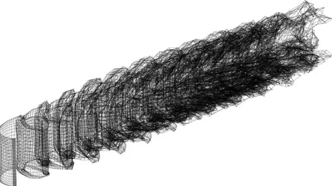
Rotor forces are evaluated from tabulated lift and drag airfoil data. The wake is discretized with vortex line elements, which are shed at the blades trailing edge during every time step and then undergo free convection behind the rotor (Fig. 4). The vortex elements are de-singularized using the van Garrel’s cut off method [35] with the vortex core size, taking into account viscous diffusion via the vortex core size that is modeled through the kinematic viscosity ν, a turbulent vortex viscosity coefficient δv and a time offset parameter Scusing Eq. (1).





1

03

.

5

























c

S

t

r

The effects of unsteady aerodynamics and dynamic stall are introduced via the ATEFlap aerodynamic model [36-37] that reconstructs lift and drag hysteresis curves from a decomposition of the lift polars. The implemented ATEFlap formulation has been further adapted to work under the intricate conditions of VAWT exhibiting large fluctuations of the angle of attack when rotating at low TSR [38].

prevent the computational cost from growing exponentially over time different wake reduction schemes (for VAWT and HAWT) are implemented [36-39].

The main parameters used in the LLFVW simulation of this study are given in Tab. 1. The azimuthal discretization was chosen to achieve a compromise between computational efficiency and accuracy. The wake was fully resolved for 12 revolutions, to obtain high quality results in the wake region, after which it was truncated. The blade was discretized into 21 panels using sinusoidal spacing to obtain a higher resolution in the tip region where the largest gradients in circulation are to be expected. The vortex time offset and the turbulent viscosity parameters were chosen so that the initial core size is large enough to prevent the simulation from diverging during the blade/wake interaction around the 270° azimuthal position, but small enough not to dampen the free wake induction onto the rotor blades and large enough not to cause the simulation to blow up due to the singularity in the Biot-Savart equation. Such an internal calibration of the vortex parameters is necessary for each turbine that is simulated and is achieved by comparing azimuthal distributions of induced velocities and blade forces over a range of these parameters.

The simulation was carried out over 16 revolutions resulting in 1152 time steps

Figure 4 - SNAPSHOT OF THE LLFVW SIMULATION AFTER 12 ROTOR REVOLUTIONS.

On a single workstation (3.3 GHz Intel Xeon 1230 v2, 8Gb ram, NVidia GTX1070 GPU) the wall clock-time required for the simulation was 196s, which reduces the runtime of the LLFVW simulation by more than 4 orders of magnitude over that of the CFD calculation. The ratio of the actual computational cost of the LLFVW and RANS simulations is probably more than 6 orders, due to the use of 8,144 cluster nodes for the RANS simulation. However, it is difficult to quantify this ratio more precisely because the processor type and architecture used by the two simulations is substantially different.

Airfoil polar data

Using accurate and high quality airfoil polar data is pivotal to obtain accurate results with the LLFVW method. Such data was obtained using the process explained in the following:

To account for the virtual camber effect [29], a virtual airfoil geometry was obtained from the NACA0021 geometry using the conformal transformation technique (Fig. 5) based on the chord-to-radius ratio, as described in [40].

Lift and drag polars (Fig. 6) of the virtual airfoil were then obtained in a Reynolds number range between 100.000 and 1.000.000 using XFoil [41] with an NCrit value of 9 and forced

transition at the leading edge of the pressure and suction side. In a different publication of the authors [5] it was shown that, besides modeling the dynamic stall, a smooth extrapolation of the polar data in the post stall region is critical to obtain high quality simulation results (e.g. [42]).

Figure 5 - GEOMETRY OF THE VIRTUAL AIRFOIL COMPENSATED FOR THE VIRTUAL CAMBER EFFECT.

Figure 6 - LIFT POLARS OF THE VIRTUAL AIRFOIL EXTRAPOLATED WITH THE MONTGOMERIE METHOD. Table 1 - SIMULATION PARAMETERS OF LLFVW IN QBlade.

Inflow 9 m/s

Azimuthal discretization 5°

Blade discretization 21 (sinusoidal)

Full wake length 12

Vortex time offset 0.0001s

Turbulent Vortex Viscosity 100

RESULTS

Torque profile

The availability of the resolved flow field past the rotor with both approaches, enables the investigation of both local flow phenomena, such as wake patterns behind the rotor, and the assessment of integral performance metrics key to design, such as the periodic torque profile over one revolution.

The impact of the effects due to finite-length blade on the periodic torque profile is analyzed first. To this aim, the reduction of the torque coefficient moving from midspan towards the tip was evaluated in terms of instantaneous torque coefficient per unit blade length (Cmz), defined by Eq. (2), in

which Tzdenotes the instantaneous torque per unit blade length

at the considered z position, and U∞ and ρ∞ denote the

freestream values of wind speed and air density, respectively.

2 2 2 1

c U T

C z

mz

 



 (2)

The periodic profiles of the torque coefficient per unit length at different span positions along the blade for the CFD and the LLFVW simulations are shown in Fig. 7 and Fig. 8, respectively. In the figures, the “0%” mark corresponds to midspan while the “100%” mark corresponds to the tip section.

One notes that the agreement between the torque profiles obtained with the two approaches in the upwind part of the revolution (i.e. from ϑ=0° to ϑ=180°) is generally good.

The torque peak values are consistent both in terms of amplitude and angular location. The blades are characterized by a predominantly 2D flow with negligible impact of tip flow effects up to 60% of the semispan. The curves at 0%, 20%, 40% and 60% are almost superimposed in both cases, while the efficiency reduction is clearly visible starting from 80% semispan. Moreover, in both cases the azimuthal position of the torque peak occurs later in the cycle as one moves towards the tip, with a shift between the 0% and 97.5% sections of about 5°. The torque reduction predicted by the two codes is comparable also at the spanwise positions closer to the tip, except for the section very close to the tip (99%), where the LLFVW is not able to predict the abrupt reduction of the torque and its negative values.

Figure 7 - CFD MOMENT COEFFICIENT vs. AZIMUTHAL ANGLE: VARIATION AT DIFFERENT SPAN LENGTHS.

Figure 8 - LLFVW MOMENT COEFFICIENT vs. AZIMUTHAL ANGLE: VARIATION AT DIFFERENT SPAN LENGTHS.

Two reasons for this discrepancy can be identified. One is that the spanwise discretization of LLFVW is much coarser than that of the CFD setup. Due to this, in the LLFVW simulation, the local moment coefficient, very close to the tip, is only interpolated, and not explicitly calculated at the respective position. The other reason is that the flow in the tip region is highly 3-dimensional due to the influence of the tip vortex. One of the main assumptions of the LLFVW method is that, when blade forces are evaluated using airfoil data, the flow on the blade surface is 2-dimensional. Even though the 3-dimensional flow in the tip region affects the inflow vectors in the virtual airfoil planes of the LLFVW method, and thereby has an effect on the generated lift and drag, the inherent simplification of the physics in this method leads to inaccurate estimates when assumptions are violated. To give an estimate of the 2D and 3D flow regions on the blade Fig. 9 shows their extensions for three angular positions close to the torque peak. In the rear of the suction side, the region of separated flow increases moving from ϑ=60° to ϑ=120°, and the downwash effect due to the tip flows increases as well.

As a result, at ϑ=60° a highly 3D flow region covers about 7% of the blade length in the tip region, while this region increases up to 15% of the blade semispan at ϑ=120°.

In the downwind position of the blade trajectory, the agreement of the torque profiles of the 2 codes is slightly poorer, although the mean torque values are still comparable, similarly to the magnitude of the torque reduction along the blade span. More specifically, although a fairly good agreement of the two codes is observed in the profiles at the spanwise positions above 90% semispan (except for the section at 99% semispan, for the reasons provided above), significant discrepancies occur around ϑ=240°, where the LLFVW torque at 90% semispan is significantly higher than that of the RANS analysis, and ϑ=270°, where the LLFVW torque is instead visibly smaller. To assess the impact of 3D effects from an aggregate point of view, the overall torque coefficient Cm of the

3D rotor defined by Eq. 3 was analyzed.



 2 0

2

H

mz

m C dz

H

C (3)

Figure 10 compares the mean 3D torque profiles obtained with the CFD analysis and the corresponding estimate obtained with the LLFVW code. The figure also provides the results of the 2D simulations of the same rotor [27], which were performed to provide the “ideal” torque of a blade with infinite span, i.e. without any secondary effects at the blade tip.

The comparison of these torque profiles shows that the “ideal” 2D torque and the 3D torque profiles are characterized by similar patterns. Since the tip losses affect only a marginal portion of the blade, no substantial modifications to the shape of the torque curve can be observed, but only a slight reduction in amplitude. For both numerical methods, the relative maxima occur at the same azimuthal positions, with a larger reduction in the upwind part of the revolution. Conversely, when the angle of attack to the airfoil is small (i.e. 0°<ϑ<40° and 150°<ϑ<210°), the 2D and 3D curves are almost superimposed. An overall good agreement of CFD and LLFVW results in the estimation of the torque modification due to the finite-blade span is noticed.

Figure 10 - MOMENT COEFFICIENT vs. AZIMUTHAL ANGLE: 2D SIMULATIONS COMPARED TO THE AVERAGE 3D

PROFILES.

Detailed flow field analyses

In this section, the 3D flow field resulting from the interaction of the rotor and the oncoming wind is analyzed in detail. Main flow structures are described in terms of velocity and vorticity, in order to highlight the main aerodynamic phenomena occurring during the revolution.

The planes used for the comparative analysis are schematically displayed in Fig. 11.

Fluid structures were investigated in the three Cartesian plane sets, at various distances from the rotor. More specifically, the following planes were considered:

• Horizontal X-Y planes: five positions along the blade semispan, starting from midspan (z/H=0) to the tip (z/H=1);

• Vertical Y-Z planes: four positions downstream the rotor, equally spaced by half rotor diameter (0.5D), starting from the rotor axis (x/D=0);

• Vertical X-Z planes: three lateral positions at 0.6R, 0.8R

and 0.9R from the rotor axis.

Figure 11 - PLANES USED FOR THE COMPARITIVE ANALYSIS OF VELOCITY AND VORTICITY CONTOURS.

In all of the following figures, LLFVW results are depicted in the left subplots, while the CFD ones are reported in the right subplots.

A comparison of the front views of the fields of the velocity modulus on the vertical Y-Z planes downstream of the rotor is shown in Fig. 12. Here the blade is positioned at the azimuthal position of maximum Cm (ϑ≈90°) and only half of the rotor

height is shown, i.e. the upper blade semispan. The rectangular area swept by the blade is highlighted by light grey lines and the blade is shadowed in dark grey.

reduction of velocity can be observed in the wake, whose shape becomes more regular, symmetric and similar to the rotor swept area moving away from the rotor. At the streamwise position of the rotor axis (x/D=0) the velocity deficit is asymmetric, with a higher deficit in the windward region of the wake, i.e. in the left side of the turbine frontal area.

Figure 12 - COMPARISON OF VELOCITY CONTOURS BETWEEN LLFVW (LEFT) AND CFD (RIGHT) ON Y-Z

PLANES AT ϑ=90° FOR DIFFERENT DISTANCES

DOWNSTREAM OF THE AXIS.

At x/D=0, the flow non-uniformity is marked also in the spanwise direction, since it affects about 40% of the blade semispan. At x/D=0.5 the effects of the tip vortex at the top right corner can be also noticed, which determines a distortion of the wake. A notable similarity of the regions of accelerated flow can be observed at all positions. Few discrepancies between the two solution sets can be however noticed, mainly related to a widening of the velocity deficit above the rotor with the LLFVW and a slightly larger instability of the wake at

x/D=1.5. Figure 13 shows the top views of the velocity fields on the horizontal X-Y planes at different semispan positions. The blade is again at ϑ=90° and its trajectory is indicated by the circular lines (the rotation is counter-clockwise). Remarkable agreement is between the two solutions is observed again. At

midspan the wake is asymmetric, as already seen in Fig. 12, and remains almost unaltered up to 60% of the semispan.

Figure 13 - COMPARISON OF VELOCITY CONTOURS BETWEEN LLFVW (LEFT) AND CFD (RIGHT) ON X-Y

PLANES AT ϑ=90° FOR DIFFERENT SPAN POSITIONS.

The CFD results show a wider area of low velocity upstream of the rotor in reason of the higher energy extraction by the turbine, as also indicated by the larger values of the torque coefficient Cmz in Fig. 7. At z/H=0.8, a global attenuation

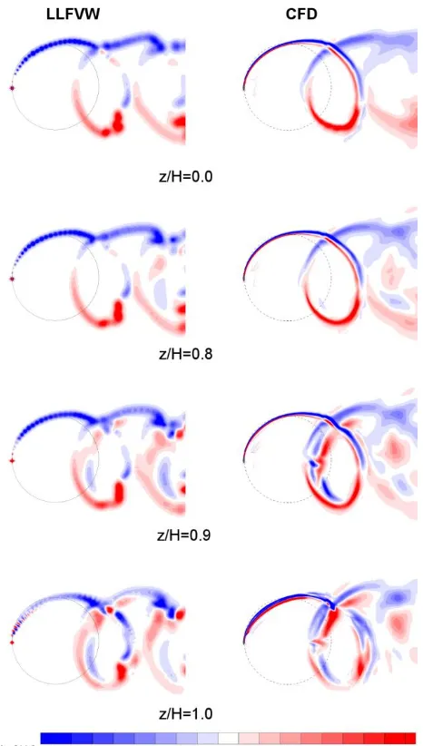
To analyze the tip vortex flow and its interaction with the blade wake, the vorticity field is examined. Figure 14 shows contour slices of the z-component of the flow vorticity on the considered horizontal X-Y planes when the blade is at ϑ=90°.

Figure 14 - COMPARISON OF Z-VORTICITY CONTOURS BETWEEN LLFVW (LEFT) AND CFD (RIGHT) ON X-Y

PLANES AT ϑ=90° FOR DIFFERENT SPAN POSITIONS.

Overall, good agreement in the wake behavior was found when comparing LLFVW and CFD solutions. These vorticity contours show that, even though the resemblance of the wake behavior predicted by the two methods is good, the wakes of the CFD solution are initially thinner. One of the reasons for this could be that the LLFVW method does not take into account the shape of the blade, and also that the mesh density of the CFD set-up is notably higher.

On the other hand, the vortices shed by the blade shortly after ϑ=90° appear to be resolved more sharply by the LLFVW method, since such approach has very low dissipation affecting

the free convection of vorticity. Further inspection of the LLFVW and CFD solutions suggests that the differences between the two approaches increase from midspan towards the tip. The z-vorticity generated by the tip vortices appears to be stronger when using the CFD method, rather than the LLFVW. This could be due to the much coarser grid used at the blade tip in the LLFVW simulation.

Figure 15 compares the contours of the y-component of the flow vorticity on different vertical X-Z planes at ϑ=90°. Half of the rotor height is shown and the lateral view of the virtual cylinder swept by the blade is highlighted by horizontal and vertical black straight lines. A good similarity of the two simulations is observed in all considered planes.

Note also that the fluid leaking at the tip generates a vortex that leaves the blade and is convected downstream. The vortex expansion due to its progressive deceleration makes it large enough to enter the virtual cylinder swept by the blade and affect a fairly large portion of the blade interacting with it in the downwind half of the revolution, as already shown in Fig. 7 and Fig. 8. Three different vortices, generated during as many revolutions, are visible in the results of both approaches.

Figure 15 - COMPARISON OF Y-VORTICITY CONTOURS BETWEEN LLFVW (LEFT) AND CFD (RIGHT) ON X-Z

PLANES AT ϑ=90° FOR DIFFERENT LATERAL POSITIONS.

As already highlighted in Fig. 14, the lower dissipation of the LLFVW method preserves the intensity of the vortices downstream the rotor, which are instead dissipated faster in the CFD solution.

The CFD solution shows a high-velocity zone in the blade wake at all span heights, which is not present in the LLFVW solution.

Figure 16 - COMPARISON OF VELOCITY CONTOURS BETWEEN LLFVW (LEFT) AND CFD (RIGHT) ON X-Y

PLANES AT ϑ=270° FOR DIFFERENT SPAN POSITIONS.

Also in this circumstance, the reason should be related to the physical thickness of the airfoil, which is accounted for only in the CFD method.

Figure 17 shows contour slices of the z-component of the flow vorticity at five spanwise positions at the azimuthal position ϑ=270°. Similarly to the ϑ=90° case, good agreement on the behavior of the blade’s wake is generally found between the LLFVW and CFD solutions. As soon as they are detached from the blades, wakes predicted by the CFD solution are sharper than those of LLFVW, suggesting a slower wake diffusion of the wake predicted by CFD. On the other hand, the

shed vortices behind the trailing edge are resolved more sharply by the LLFVW, which limits their coalescence.

Figure 17 - COMPARISON OF Z-VORTICITY CONTOURS BETWEEN LLFVW (LEFT) AND CFD (RIGHT) ON X-Y

PLANES AT ϑ=270° FOR DIFFERENT SPAN POSITIONS.

Overall, the z-vorticity generated by the tip vortices is stronger when using the CFD method, thus generating a stronger wake. Finally, the differences between the two approaches increase from midspan towards the tip.

Fig. 19. Beside possible differences in the resolution of the wake evolution, this behavior can be physically related to what already pointed out for the profiles of the torque coefficient of Fig. 7 and Fig. 8.

The predicted torque in the upwind half of the rotation is very similar, leading to similar predictions of the energy extraction and similar velocity deficit at x/D=0. Conversely, the discrepancies in the torque prediction at the angular position of

ϑ=240° and ϑ=270° lead to an analogous behavior of the wake profiles. Indeed, the differences are significant for y/D<0, while similar trends are obtained for y/D>0, corresponding to the windward half of the rotation. Notwithstanding this, it can be pointed out that the overall amplitudes of the velocity deficit are coherent for all the analyzed locations.

Figure 18 - AVERAGE VELOCITY PROFILE COMPARISON BETWEEN LLFVW AND CFD ON X-Y PLANES AT DIFFERENT

SPAN HEIGHTS AT X/D=0 (A) AND X/D=1 (B).

Figure 19 - RELATIVE ERROR OF AVERAGE VELOCITY PREDICTED BY CFD AND LLFVW ALONG THE SPAN

HEIGHT AT X/D=0 AND X/D=1.

The level of agreement between the velocity predictions in the wake was assessed quantitatively by calculating the percentage difference between the CFD and LLFVW profiles.

The values were averaged along the y-direction in the range -1<y/R<1 and the percentage differences at various blade heights are reported in Fig. 19. These results confirm that the differences between the two predictions are very low (below 1.5%) for most of the wake region and tend to increase up to roughly 5% only in proximity of the tip. At each span position, the difference between the two codes is lower at x/D=0 than at

x/D=1.

CONCLUSIONS

In this study, the 3D numerical simulation of a single blade in Darrieus-like motion was carried out with both a highly refined, time-dependent CFD model and a LLFVW code.

A CFD mesh featuring a very fine discretization level was used to accurately solve the flow field, in order to provide highly resolved data to assess the prediction capabilities of the LLFVW method.

The comparison showed an extremely promising agreement between the results. In particular, the investigation of the torque reduction due to finite-blade effect confirmed the consistency on the two approaches in predicting the efficiency reduction as a function of the blade span. The discrepancies in the LLFVW curves are related to a slight underestimation of the torque peak and to the presence of a torque deficit at the azimuthal position

ϑ=270°. A comparative analysis of the velocity and vorticity contours was then carried out to better highlight the capability of predicting the most relevant flow features. The rotor wake analysis showed similar velocity patterns and fairly good agreement of the vorticity fields.

is more than 6 orders of magnitude lower than the one of the CFD simulation. However, thanks to the constant increase of the hardware performance, the possibility of performing accurate 3D CFD simulations is, and will be, pivotal to provide high-quality data for the validation and calibration of such low-order models.

ACKNOWLEDGMENTS

The authors acknowledge use of Hartree Centre resources in this work. Part of the reported simulations were also performed on two other clusters. One is POLARIS (coordinated by the Universities of Leeds and Manchester) part of the N8 HPC facilities provided and funded by the N8 consortium and EPSRC (Grant No.EP/K000225/1). The other resource is the HEC cluster of Lancaster University, which is also kindly acknowledged. Finally, thanks are due to Prof. Ennio Antonio Carnevale of the Università degli Studi di Firenze for supporting this research.

REFERENCES

[1] Paraschivoiu, I., 2002, Wind turbine design with emphasis on Darrieus concept, Polytechnic International Press, Montreal, Canada.

[2] Mohamed, M.H., 2014, “Aero-acoustics noise evaluation of H-rotor Darrieus wind turbines,” Energy, 65(1), pp. 596-604.

[3] Balduzzi, F., Bianchini, A., Carnevale, E.A., Ferrari, L. and Magnani, S., 2012, “Feasibility analysis of a Darrieus vertical-axis wind turbine installation in the rooftop of a building,” Applied Energy, 97, pp. 921–929.

[4] Bianchini, A., Ferrari, L. and Magnani, S., 2012, “Energy-yield-based optimization of an H-Darrieus wind turbine,”

Proceedings of the ASME Turbo Expo 2012, Copenhagen (Denmark), June 11-15, 2012.

[5] Marten, D., Bianchini, A., Pechlivanoglou, G., Balduzzi, F., Nayeri, C.N., Ferrara, G., Paschereit, C.O. and Ferrari, L., 2016, “Effects of airfoil's polar data in the stall region on the estimation of Darrieus wind turbines performance,”

J. of Engineering for Gas Turbines and Power, 139(2), pp. 022606-022606-9.

[6] Marten, D., Lennie, M., Pechlivanoglou, G., Nayeri, C.D. and Paschereit, C.O., 2016, "Nonlinear Lifting Line Theory Applied To Vertical Axis Wind Turbines: Development of a Practical Design Tool," Proc. of the ISROMAC Conference, Honolulu, Hawaii, 2016.

[7] Dossena, V., Persico, G., Paradiso, B., Battisti, L., Dell’Anna, S., Brighenti, A. and Benini, E., 2015, “An Experimental Study of the Aerodynamics and Performance of a Vertical Axis Wind Turbine in a Confined and Non-Confined Environment,” Proc. of the ASME Turbo Expo 2015, Montreal, Canada, June 15-19, 2015.

[8] Bachant, P. and Wosnik, M., 2015, “Characterising the near-wake of a cross-flow turbine,” Journal of Turbulence,

16(4), pp. 392–410.

[9] Bianchini, A., Balduzzi, F., Bachant, P., Ferrara, G. and Ferrari, L., 2017, “Effectiveness of two-dimensional CFD simulations for Darrieus VAWTs: a combined numerical and experimental assessment,” Energy Conversion and Management, 136(15 March 2017), pp. 318-328.

[10] Balduzzi, F., Bianchini, A., Maleci, R., Ferrara, G. and Ferrari, L., 2016, “Critical issues in the CFD simulation of Darrieus wind turbines,” Renewable Energy, 85(01), pp. 419-435.

[11] Balduzzi, F., Bianchini, A., Ferrara, G., Ferrari, L., 2016, “Dimensionless numbers for the assessment of mesh and timestep requirements in CFD simulations of Darrieus wind turbines,” Energy, 97(15 February 2016), pp. 246-261.

[12] Balduzzi, F., Bianchini, A., Gigante, F.A., Ferrara, G., Campobasso, M.S. and Ferrari, L., 2015, “Parametric and Comparative Assessment of Navier-Stokes CFD Methodologies for Darrieus Wind Turbine Performance Analysis,” Proc. of the ASME Turbo Expo 2015, Montreal, Canada, June 15-19, 2015.

[13] Lam H.F. and Peng, H.Y., 2016, “Study of wake characteristics of a vertical axis wind turbine by two- and three-dimensional computational fluid dynamics simulations,” Renewable Energy, 90(May 2016), pp. 386-398.

[14] Raciti Castelli, M., Pavesi, G., Battisti, L., Benini, E. and Ardizzon, G., 2010, “Modeling strategy and numerical validation for a Darrieus vertical axis micro-wind turbine,”

Proc. of the ASME IMECE 2010, Vancouver, British Columbia, Canada, November 12-18, 2010.

[15] Untaroiu, A., Wood, H.G., Allaire, P.E. and Ribando, R.J., 2011, “Investigation of Self-Starting Capability of Vertical Axis Wind Turbines Using a Computational Fluid Dynamics Approach,” ASME Journal of Solar Energy Engineering, 133(November 2011), pp. 041010-1-8. [16] Alaimo, A., Esposito, A., Messineo, A., Orlando, C. and

Tumino, D., 2015, “3D CFD Analysis of a Vertical Axis Wind Turbine,” Energies, 8, pp. 3013-3033.

[17] De Marco, A., Coiro, D.P., Cucco, D. and Nicolosi F., 2014, “A Numerical Study on a Vertical-Axis Wind Turbine with Inclined Arms,” 2014, International Journal of Aerospace Engineering, pp. 1-14.

[18] Raciti Castelli, M. and Benini, E., 2012, “Effect of Blade Inclination Angle on a Darrieus Wind Turbine,” ASME Journal of Turbomachinery 2012; 134(May 2012): 031016-1-10.

[19] Orlandi, A., Collu, M., Zanforlin, S. and Shires, A., 2015, “3D URANS analysis of a vertical axis wind turbine in skewed flows,” J. of Wind Engineering and Industrial Aerodynamics,147(December 2015), pp. 77-84.

the ASME Turbo Expo 2015, Charlotte, USA, June 27-30, 2017.

[21] Bianchini, A., Balduzzi, F., Ferrara, G., Ferrari, L., Persico, B., Dossena, V. and Battisti, L., 2017, “A combined experimental and numerical analysis of the wake structure and performance of a H-shaped Darrieus wind turbine,” Proc. of the 1st _{GPPS Forum, Zurich,}

Switzerland, January 16-18, 2017.

[22] Menter, F.R., “Two-equation Turbulence-models for Engineering Applications,” AIAA Journal, 32(8), pp. 1598-1605.

[23] Campobasso, M.S., Piskopakis, A, Drofelnik, J. and Jackson, A., 2013, “Turbulent Navier-Stokes Analysis of an Oscillating Wing in a Power Extraction Regime Using the Shear Stress Transport Turbulence Model,” Computers and Fluids, 88, pp. 136-155.

[24] Drofelnik, J. and Campobasso, M.S., 2016, “Comparative Turbulent Three-Dimensional Navier-Stokes Hydrodynamic Analysis and Performance Assessment of Oscillating Wings for Renewable Energy Applications,”

International Journal of Marine Energy, 16, pp. 100-115. [25] Campobasso, M.S., Gigante, F. and Drofelnik, J.,

“Turbulent Unsteady Flow Analysis of Horizontal Axis Wind Turbine Airfoil Aerodynamics Based on the Harmonic Balance Reynolds-Averaged Navier-Stokes Equations,” Proc. of the ASME Turbo Expo 2014, Düsseldorf, Germany, June 16-20, 2014.

[26] Campobasso, M.S. and Baba-Ahmadi, M.H., 2012, “Analysis of Unsteady Flows Past Horizontal Axis Wind Turbine Airfoils Based on Harmonic Balance Compressible Navier-Stokes Equations with Low-Speed Preconditioning,” J. of Turbomachinery, 134(6), pp. 061020-1-13.

[27] Bianchini, A., Balduzzi, F., Ferrara, G. and Ferrari, L., 2017, “Aerodynamics of Darrieus wind turbines airfoils: the impact of pitching moment,” J. Engineering for Gas Turbines and Power, 139(4), pp. 042602-1-12.

[28] Gigante, F.A., Balduzzi, F., Bianchini, A., Minghan, Y., Ferrara, G., Campobasso, M.S. and Ferrari, L., 2017, “On the Application of the Reynolds-Averaged Navier-Stokes Equations and the Shear Stress Transport Turbulence Model for the Performance Estimation of Darrieus Wind Turbines,” paper submitted for publication to J. of Wind Engineering and Industrial Aerodynamics.

[29] Rainbird. J., Bianchini, A., Balduzzi, F., Peiro, J., Graham, J.M.R., Ferrara, G. and Ferrari, L., 2015, “On the Influence of Virtual Camber Effect on Airfoil Polars for Use in Simulations of Darrieus Wind Turbines,” Energy Conversion and Management, 106(December 2015), pp. 373-384.

[30] Campobasso, M.S., Drofelnik, J., Gigante, F., 2016, “Comparative Assessment of the Harmonic Balance Navier-Stokes Technology for Horizontal and Vertical Axis Wind Turbine Aerodynamics,” Computers and Fluids, 136, pp. 354-370.

[31] http://community.hartree.stfc.ac.uk/wiki/site/admin/ resources.html, last accessed 10/05/2016.

[32] Marten, D., Pechlivanoglou, G., Nayeri, C.N. and Paschereit, C.O., 2010, “Integration of a WT Blade Design tool in XFOIL/XFLR5,” Proceedings of DEWEK 2010, 17-18 November 2010, Bremen, Germany.

[33] Marten, D., Wendler, J., Pechlivanoglou, G., Nayeri, C.N. and Paschereit, C.O., 2013, "QBlade : An Open Source Tool For Design And Simulation Of Horizontal And Vertical Axis Wind Turbines," IJETAE, 3 special issue, pp. 264–269.

[34] Van Garrel, A., 2003, “Development of a wind turbine aerodynamics simulation module,” tech. rep.

[35] Marten, D., 2016, "QBlade Guidelines v0.95", tech. rep., TU Berlin.

[36] Marten, D., Lennie, M., Pechlivanoglou, G., Nayeri, C.D. and Paschereit, C.O., 2015, "Implementation, Optimization and Validation of a Nonlinear Lifting Line Free Vortex Wake Module within the Wind Turbine Simulation Code QBlade," Journal of Engineering for Gas Turbines And Power, 138(7), pp. 072601-1-10. [37] Marten, D., Pechlivanoglou, G., Nayeri, C.N. and

Paschereit, C.O., 2016, “Nonlinear Lifting Line Theory Applied To Vertical Axis Wind Turbines: Development of a Practical Design Tool,” Proc. of the ISROMAC 2016, Hawaii, USA.

[38] Bergami, L. and Gaunaa, M., 2012, “ATEFlap Aerodynamic Model, a dynamic stall model including the effects of trailing edge flap deflection,” tech. rep., DTU. [39] Wendler, J., Marten, D., Pechlivanoglou, G., Nayeri, C.N.

and Paschereit, C.O., 2016, “Implementation and Validation of an Unsteady Aerodynamics Model for Horizontal and Vertical Axis Wind Turbines within the Simulation Tool QBlade,” Proc. of the ASME Turbo Expo 2016, June 13- 17, Seoul, South Korea.

[40] Bianchini, A., Balduzzi, F., Rainbird, J., Peiro, J., Graham, J M.R., Ferrara, G. and Ferrari, L., 2015, “An Experimental and Numerical Assessment of Airfoil Polars for Use in Darrieus Wind Turbines. Part I - Flow Curvature Effects,” J. Engineering for Gas Turbines and Power, 138(3), pp. 032602-1-10.

[41] Drela, M., and Giles, M., 1989, “Viscous-Inviscid Analysis of Transonic and Low Reynolds Number Airfoils,” AIAA Journal, 25(10), pp. 1347-1355.