R E S E A R C H A R T I C L E
Open Access
Comparison of Bayesian and frequentist
group-sequential clinical trial designs
Nigel Stallard
1*, Susan Todd
2, Elizabeth G. Ryan
3and Simon Gates
3Abstract
Background: There is a growing interest in the use of Bayesian adaptive designs in late-phase clinical trials. This includes the use of stopping rules based on Bayesian analyses in which the frequentist type I error rate is controlled as in frequentist group-sequential designs.
Methods: This paper presents a practical comparison of Bayesian and frequentist group-sequential tests. Focussing on the setting in which data can be summarised by normally distributed test statistics, we evaluate and compare boundary values and operating characteristics.
Results: Although Bayesian and frequentist group-sequential approaches are based on fundamentally different paradigms, in a single arm trial or two-arm comparative trial with a prior distribution specified for the treatment difference, Bayesian and frequentist group-sequential tests can have identical stopping rules if particular critical values with which the posterior probability is compared or particular spending function values are chosen. If the Bayesian critical values at different looks are restricted to be equal, O’Brien and Fleming’s design corresponds to a Bayesian design with an exceptionally informative negative prior, Pocock’s design to a Bayesian design with a non-informative prior and frequentist designs with a linear alpha spending function are very similar to Bayesian designs with slightly informative priors.
This contrasts with the setting of a comparative trial with independent prior distributions specified for treatment effects in different groups. In this case Bayesian and frequentist group-sequential tests cannot have the same stopping rule as the Bayesian stopping rule depends on the observed means in the two groups and not just on their difference. In this setting the Bayesian test can only be guaranteed to control the type I error for a specified range of values of the control group treatment effect.
Conclusions: Comparison of frequentist and Bayesian designs can encourage careful thought about design parameters and help to ensure appropriate design choices are made.
Keywords: Adaptive design, Interim analysis, Type I error rate, Sequential analysis, Sequential design
Background
An increasing desire for efficiency in clinical trials has led to growing interest in adaptive designs. Frequentist group-sequential designs enable interim analyses to be performed during the conduct of a clinical trial with-out inflation of the overall type I error rate [1]. With an increased application of Bayesian methods in clinical trials, a number of researchers have proposed Bayesian group sequential methods [2,3].
*Correspondence:n.stallard@warwick.ac.uk
1Statistics and Epidemiology, Division of Health Sciences, Warwick Medical School, University of Warwick, Coventry, UK
Full list of author information is available at the end of the article
Not all proponents of Bayesian sequential designs con-sider exact control of the type I error rate essential [4]. Some, however, have suggested that the stopping rules for Bayesian group sequential designs should also be cho-sen in such a way that the frequentist type I error rate is controlled [2,5,6], particularly in the setting of phase III or late phase II clinical trials, when it is often consid-ered desirable to control the risk of a false positive result, that is an erroneous conclusion that a new treatment is efficacious.
There are a number of published examples of trials using a Bayesian stopping rule chosen to control the type I error
rate. Hueber et al. [7] (see also [8] for additional statis-tical details) describe a Bayesian group-sequential trial comparing secukinumab with placebo for the treatment of Crohn’s disease. The outcome is the change in Crohn’s Disease Activity Index (CDAI), which was taken to be nor-mally distributed. Prior distributions were specified sep-arately for the placebo and secukinumab effects, with the former being informative and the latter non-informative. Analyses were planned after 30 and 60 patients, when the trial could be stopped if both (i) the posterior probability that secukinumab was superior to the placebo exceeded 95%, and (ii) there was at least a 50% posterior proba-bility that the change in CDAI due to secukinumab was superior to that for placebo by at least fifty. The type I error rate for this design was calculated using the R pack-agegsbDesign[9] and shown to be 1.2% if the change in CDAI due to placebo was as anticipated.
A Bayesian group-sequential trial with a binary pri-mary outcome is described by Wilber et al. [10]. This randomised trial compared antiarrhythmic drug therapy with catheter ablation for the treatment of paroxysmal atrial fibrillation. The primary outcome was the observa-tion of protocol-defined treatment failure. Analyses were planned after 150, 175, 200 and 230 patients, with a stop-ping rule based on the posterior probability of superiority of the experimental treatment over the control exceeding 98%, giving a type I error rate of 0.025.
The increasing use of Bayesian sequential designs that control the frequentist type I error rate has led to a grow-ing body of work compargrow-ing Bayesian and frequentist group sequential trial methods [3,5,8,11–14]. This paper adds to this work. In contrast to some authors who draw comparisons between underlying Bayesian and frequen-tist paradigms, our focus is a practical one, in which we compare Bayesian and frequentist group sequential tests in terms of their boundary values and operating charac-teristics. We consider specifically the setting of normally distributed data or test statistics. This facilitates compar-ison between Bayesian and frequentist group sequential methods as the latter have been largely developed in this setting.
We consider separately Bayesian designs in which a single treatment effect is considered, either in a single-arm trial or with a prior specified directly for the dif-ference between experimental and control treatments, and in which treatment effects have independent prior distributions. In the one-parameter setting frequentist and Bayesian group-sequential designs can be identical if sufficient flexibility in choice of design parameters is allowed [12], and we show that frequentist and Bayesian group-sequential designs may be very similar for common choices of stopping rules. In the two-parameter setting we show that the frequentist and Bayesian designs can-not correspond, and show that in this case the Bayesian
group-sequential designs can only control the type I error rate for specified values of the control group treatment effect.
Methods
Notation and problem formulation
Single arm trials with normally distributed data
Suppose we conduct a group-sequential single-arm clin-ical trial of some experimental treatment with up to K
analyses of a single sample of normally distributed data with a cumulative total ofnk observations at lookk,k = 1,. . .,K.
At each look the data observed up to that point will be analysed and a decision made whether or not to continue to the next look. We will only consider stopping the trial for a positive result, that is for efficacy. Additional stop-ping for futility is considered in the “Discussion” section.
Denoting by Yi the observed value for patient i, we will assume this is normally distributed with meanθ and known varianceσ2. We wish to draw inference onθ and will assume that parameterisation is such thatθ = 0 cor-responds to the experimental treatment being of equal efficacy to some specified reference value or standard treatment effect, with positive values ofθ(and hence ofYi) indicative of superiority of the experimental treatment.
LetY¯k = ni=k1Yi/nk denote the mean value from the cumulative sample at lookk. This is the sufficient statis-tic forθ at lookk. It is helpful to write the distribution in terms of the inverse of the variance, known as the infor-mation, and set Ik = nk/σ2. We then haveY¯1,. . .,Y¯K multivariate normal with
⎛ ⎜ ⎝ ¯ Y1 .. . ¯ YK ⎞ ⎟ ⎠∼N
⎛ ⎜ ⎜ ⎜ ⎝ ⎛ ⎜ ⎝ θ .. . θ ⎞ ⎟ ⎠, ⎛ ⎜ ⎜ ⎜ ⎝
I1−1 I2−1 · · · IK−1 I2−1 I2−1 · · · IK−1
..
. ... . .. ...
IK−1 IK−1 · · · IK−1
⎞ ⎟ ⎟ ⎟ ⎠ ⎞ ⎟ ⎟ ⎟ ⎠ (1)
with a similar multivariate normal distribution for the standardised test statistics,Y¯1√I1,. . .,Y¯K√IK.
In a frequentist setting, we will test the null hypothesis,
H0 :θ ≤ 0 against the one-sided alternative,θ >0, con-cluding that the experimental treatment is superior to the standard if this null hypothesis is rejected. The test will be based on the observed values ofY¯1,. . .,Y¯K, stopping and rejecting the null hypothesis at lookkifY¯k is sufficiently large as described in more detail below.
In a Bayesian setting, inference will be based on the pos-terior distribution for θ given the observed data. Basing the likelihood on (1), a normal prior for θ is conjugate. Given prior distribution θ ∼ N θ0,I0−1
the posterior distribution forθfollowing observation ofY¯k = ¯ykat look
θ | ¯yk ∼N
θ
0I0+ ¯ykIk
I0+Ik
, 1
I0+Ik
(2)
(see [15] Section 5.2). If this posterior distribution is suf-ficiently indicative of a positive treatment effect the trial will be stopped with the conclusion that the experimental treatment is superior to the standard or reference value. More details are given below.
The value ofI0gives a measure of the prior information. In particular, lettingI0approach 0 gives a flat improper normal prior.
Single arm trials with non-normal data
For non-normal data, tests can be based on the assumed distributional form parameterised in terms of the treat-ment effect, which will again be denoted byθ. An analytic form of the posterior distribution may be available if a conjugate prior distribution is used.
Alternatively, in many cases, ifn1,. . .,nKare sufficiently large, we can obtain an estimate θkˆ for the treatment effect based on the data at lookkwithθˆ1,. . .,θKˆ approx-imately following the multivariate normal distribution (1) for someI1,. . .,IK. It is common to use this approximate distributional form in a frequentist group-sequential test [16], enabling use of these estimates in place of the single sample means and applying methods based on the normal distribution (1) even without normally distributed data, or with normal data when the variance cannot be assumed to be known.
An illustration in the setting of a single sample of bino-mial data is given below.
Comparative trials
Suppose now we have two groups; group 0, the control group and group 1, the experimental treatment group. Let Yji denote the response from patient i in group j, assumed to be normally distributed with known variance, withYji ∼ N μj,σj2
,j = 0, 1. We wish to draw infer-ence on the treatment differinfer-ence given byθ = μ1−μ0. We will again assume larger values ofYjiare preferable so that larger values ofθcorrespond to the superiority of the experimental treatment to the control treatment.
At analysisk, suppose that we have a total ofnjk observa-tions from groupj, and letY¯jk =in=jk1Yji/njk,j=0, 1,k=
1,. . .,K. WritingIjk=njk/σj2, we haveY¯j1,. . .,Y¯jK multi-variate normal withY¯jk ∼N μj,Ijk−1and cov(Y¯jk,Y¯jk)=
Ijk−1ifk<k.
A sufficient statistic for θ at look k is Dk = ¯Y1k −
¯
Y0k, with D1,. . .,DK following the multivariate normal distribution as in (1) withIk =σ12/n1k+σ02/n0k−1.
In a frequentist setting, we will test H0 : θ ≤ 0
againstθ >0 based on the observed values ofD1,. . .,DK, stopping and rejecting the null hypothesis at look k,
concluding that the experimental treatment is superior to the control, ifDkis sufficiently large, as described in more detail below.
In a Bayesian setting, we may specify the prior distri-bution for the treatment effect in two ways. The first is to specify a prior distribution for the treatment differ-ence,θ, directly. Suppose again thatθ has a normal prior distribution withθ ∼ N θ0,I0−1
. At look k the poste-rior distribution for θ given observed valueDk = dk is given by
θ |dk∼N
θ0I0+dkIk
I0+Ik
, 1
I0+Ik
. (3)
The alternative is to specify independent prior distri-butions forμ0andμ1, update these separately to obtain posterior distributions forμ0andμ1and then use these to obtain a posterior distribution for θ. This approach is considered in detail below in the section entitled “Comparison of frequentist and Bayesian group-sequen-tial approaches - two parameter case”.
For non-normal data, or when the variance cannot be assumed known, we often again have estimates of the treatment effect,θkˆ, approximately normally distributed, so that the distributional form (1) can be used. As in the two-sample case with normally distributed data, in the Bayesian setting we can either specify a prior forθdirectly or specify independent prior distributions for treatment effects in the two groups.
Bayesian group-sequential approach
In a Bayesian sequential trial, inference at lookkwill be based on the posterior distribution forθgiven in the single group case by (2), in the two sample case when a prior distribution is specified forθdirectly by (3) and in the two sample case when prior distributions are given forμ0and μ1by the expression (10) given below.
A common approach is to stop the trial, concluding that the experimental treatment is superior to the control if the posterior probability thatθ exceeds 0 given the observed data is sufficiently large. In detail, critical values,pk,k = 1,. . .,K, will be specified and the trial will stop as soon as
Pr(θ >0|data at lookk)≥pk. (4) Considering stopping to conclude the experimental treatment is superior to the control to be equivalent to rejection of H0, the frequentist type I error rate of this Bayesian sequential procedure can be calculated by not-ing thatPr(θ > 0 | data at lookk)is a random variable since it depends on the observed data. Control of the type I error rate is thus achieved if
It has been suggested thatp1,. . .,pK should be chosen to satisfy this condition [2].
A number of alternatives to the stopping criterion (4) above have also been proposed. For example, the trial might be stopped to declare the experimental treatment superior at look k if the posterior probability that θ exceeds some specified positive target value, or the predic-tive probability that the experimental treatment would be found superior if the trial continued to the final analysis, is sufficiently large [8,17,18].
Although, in general, different values for p1,. . .,pK could be specified, often a common valuep1 = · · · =pK is used [2], with this value chosen to satisfy (5). We will consider both the general and this specific case in the examples below.
In many settings the probability on the left hand side of (5) can most easily be calculated via simulation methods [2]. In the case of single- or two-sample normally dis-tributed data considered here, since, for a specified prior distribution, the posterior probability (4) depends onY¯k, it can be calculated analytically from the joint distribution (1), for example in R using the gsbDesign[9] or code available from the first author.
Frequentist group-sequential approaches
In a frequentist setting, the null hypothesis,H0 : θ ≤ 0, will be rejected, and the trial stopped at lookkifY¯k√Ik ≥
ukfor someukin the single-sample case or ifDk
√
Ik≥uk in the two sample case. As the forms of the joint distribu-tions forY¯1,. . .,Y¯K andD1,. . .,DK are identical, we will here consider only the single-sample case.
To control the type I error rate at some specified level α, it is required to choose u1,. . .,uK with Pr(Y¯k√Ik ≥
uk, somek≤K;θ)≤αfor allθ ≤0. The form (1) means that this is satisfied if
Pr(Y¯k
Ik≥uksomek≤K;θ =0)=α. (6)
As the requirement (6) is insufficient to specify
u1,. . .,uK, a number of approaches have been proposed as described in the next two subsections.
Pocock’s test and O’Brien and Fleming’s test
Pocock [19] and O’Brien and Fleming [20] propose meth-ods with equally-spaced looks, that is, using the nota-tion introduced above, with Ik = kIK/K,k = 1,. . .,K. O’Brien and Fleming suggest stopping if Y¯kIk exceeds
some fixed value, that is taking uk = c/
√
Ik. Pocock suggests stopping if the standardised difference Y¯kIk1/2 exceeds a fixed value, that is taking uk = c. In each
case, the constant value for c is found so as to
sat-isfy (6). These values are tabulated for certain K andα [19, 20], or can be obtained from a numerical search,
noting that the probability in (6) can be expressed
in terms of the multivariate normal distribution func-tion which may be evaluated numerically, for
exam-ple in R using function pmvnorm in the mvtnorm
package [21].
Spending function approaches
Slud and Wei [22] suggest introducing greater flexibility to sequential designs that satisfy (6) by specifying the type I error rate “spent” at each look. In detail, they specifyα1≤
· · · ≤ αK = α, then obtainuk,k = 1,. . .,K, such that the probability under the null hypothesis of stopping at or before lookk, say at some lookkwithk ≤k, is equal to αk, that is
Pr(Y¯k
Ik ≥uksomek≤k;θ =0)=αk. (7)
This approach was extended by Lan and DeMets [23],
who proposed thatα1,. . .,αK be given by a functionα∗(t) of the information time, witht at look k equal toIk/IK so thatαk = α∗(Ik/IK),k = 1,. . .,K. For general choice of non-decreasing α∗ with α∗(0) = 0 andα∗(1) = α, the approaches of Slud and Wei and Lan and DeMets are equivalent providedI1,. . .,IKare specified in advance. By defining the functional form ofα∗, the Lan and DeMets approach enables calculation of u1,. . .,uK to satisfy (6) whenI1,. . .,IK are not given in advance, providing they are independent ofY¯1,. . .,Y¯K.
Lan and DeMets give forms for the spending function α∗(t) corresponding approximately to the Pocock test,
withα∗(t)=αlog(1+(e−1)t), and the O’Brien and Flem-ing test, withα∗(t)=2(1−(zα/√t)), wheredenotes the distribution function for a standard normal and zα denotes−1(1−α), the upper 100αpercentile of the stan-dard normal distribution. Exact spending functions for these tests for a given number of looks can be obtained numerically from the joint distribution (1) [24]. Alterna-tive spending function forms have been suggested [1,25], including as a special case the linear spending function α∗(t)=αt.
The stopping boundary valuesu1,. . .,uK may be com-puted recursively[1]; at lookk, supposingu1,. . .,uk−1and
I1,. . .,Ik are known, we can use the joint distribution of
¯
Y1,. . .,Y¯k for θ = 0 from (1) along with a numerical search to findukto satisfy (7). These calculations can be
performed in R using the gsBound in the gsDesign
package [26] or code available from the first author.
Examples
Example 1: Single-arm trial with normally distributed data Consider a single-arm trial with the outcome for patienti
equal toYiwithYi∼N(θ,σ2)for some knownσ. Suppose
thatθ = 0 corresponds to a null value and θ = 1 to a
worthwhile treatment effect. We will assume that the trial is conducted in up to five stages, that isK=5, with these of equal size so that the number of patients included in the firstkstages is nk = nk/K. We will further assume thatnK =10σ2. With this sample size a fixed sample size trial with a hypothesis test conducted at a two-sided 5% level would have power of approximately 90%. This gives
I1,. . .,I5=2,. . ., 10.
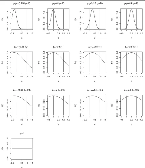
We will consider a range of prior distributions forθ. We will takeI0equal to 0 (non-informative), 0.5 and 1 (that is with weight equivalent to one twentieth and one tenth of the total information available from the trial) as well as a very informative prior distribution withI0= 20, and will takeθ0equal to−0.25, 0, 0.25 and 0.5, recalling that 0 and 1 correspond to null and worthwhile treatment effects. Density functions for the range of prior distributions con-sidered are shown in Fig.1. The prior mean,θ0, increases across the columns moving from left to right and the prior information,I0, decreases as we move down the rows. The vertical lines correspond to the null and worthwhile treat-ment effects of 0 and 1. Only one plot is given in the lowest row as whenI0=0 the prior distribution does not depend onθ0.
Example 2: Single-arm trial with binary data
Consider, as a second example, a single-arm trial with a binary outcome corresponding to success or failure for each patient. Suppose that the trial has up to four looks with 25, 50, 75 and 100 patients and assume that we wish to determine whether the true success rate, which will be denoted byπ, exceeds a control rate,π0, assumed to be 0.5, using a non-informative prior distribution forπ.
Example 3: Two-arm trial with normally distributed data The third example is a two-arm trial with up to five equally-sized stages with the outcome for patient i in groupj(j = 0, 1)equal toYij withYij ∼ N μj,σj2
for some knownσj, where we assumeσ1=σ0.
Denoting the treatment differenceμ1−μ0byθ, we will,
as in Example1above, assume thatθ = 1 represents a
worthwhile treatment effect. Assuming at stagekwe have included a total ofnkpatients in each of the two trial arms, we will setIk = nk/2σ2and, again as in Example1, take
I1,. . .,I5=2,. . ., 10.
Suppose thatμ1andμ0have independent normal prior distributions withμj ∼ N μj0,Ij−01
, with a moderately informative prior distribution for μ0with μ00 = 0 and
I00 = 0.5, and a noninformative prior distribution forμ1 withI10 =0. The treatment differenceθ thus has a non-informative prior distribution withI0=0.
Results
Comparison of frequentist and Bayesian group-sequential approaches - single parameter case
In this section we consider the setting in which we either have a single sample or are comparing two groups but specify a prior distribution for the treatment effect, θ, directly rather than giving separate prior distributions for μ1andμ0. As noted above, in this case the two-sample setting is essentially identical to the single-sample set-tings, so that we will consider only the latter specifically.
Suppose that the maximum number of looks, K, the
information at these looks,I1,. . .,IK and, for the Bayesian design, the prior distribution parameters, θ0 and I0 are specified.
The posterior distribution forθ at lookkin this case is given by (2) so that the posterior probability thatθexceeds 0 is given by
Pr(θ >0| ¯yk,Ik)=1−
−¯
ykIk−θ0I0
√
I0+Ik
. (8)
Given some choice ofp1,. . .,pK, for the Bayesian design using stopping criterion (4) expression (8) means that the trial will be stopped at lookkifY¯k√Ik ≥uBk where
uBk = −θ0I0−
√
I0√+Ik−1(1−pk)
Ik
(9)
so that the Bayesian trial, like the frequentist one, will stop wheneverY¯k, or equivalently the standardisedY¯k√Ik, is sufficiently large.
Sequential tests with generalα1,. . .,αKor p1,. . .,pK
With uBk as given by (9), let αkB = Pr(Y¯k√Ik ≥
uBksomek ≤ k;θ = 0). This may be calculated from
the multivariate normal distribution ofY¯1√I1,. . .,Y¯k
√
Ik following from (1). Settingk = Kenables analytic calcu-lation of the frequentist type I error rate for the Bayesian test.
Settingαk = αBk and constructing a frequentist design using theseα1,. . .,αKvalues will give a frequentist group-sequential boundary identical to the Bayesian one.
Similarly, given frequentist group sequential spend-ing function valuesα1,. . .,αK, we can obtainu1,. . .,uK
to satisfy (7). A Bayesian design with pk = 1 −
(−uk√Ik−θ0I0)/√I0+Ik
,k=1,. . .,K, will then be identical to this frequentist one.
Thus, as noted by Emerson et al. [12], if we allow full flexibility over the choice ofp1,. . .,pK for the Bayesian group-sequential design andα1,. . .,αK for the frequen-tist design, subject respectively to the constraint on overall type I error rate (5) or (6), the classes of frequentist group sequential and Bayesian designs are identical.
Fig. 1Densities for range of prior distributions for Bayesian sequential designs for Example 1
positive target value or the posterior predictive probabil-ity of a final positive result, the fact that both of these are monotonically increasing in Y¯k means that the stopping boundaries are again of the formY¯k√Ik ≥ uBk for some
[image:6.595.59.538.86.638.2]be monotonically increasing inY¯k, as is the case, for exam-ple, when a point null atθ =0 is compared to a ‘one-sided’ prior with support for positiveθ only.
Specific group-sequential tests: Single-arm trial with normally distributed data
Although in principle,p1,. . .,pK andα1,. . .,αK may be chosen arbitrarily, in practice, constraints may be put on the values used. In this case frequentist and Bayesian group sequential tests may not correspond. In this section we construct frequentist group-sequential designs with a linear alpha spending function and with alpha spend-ing functions correspondspend-ing to the Pocock design and the O’Brien and Fleming design, comparing these with Bayesian tests with stopping criteria given by (4) with
p1= · · · =pK.
Consider Example1above with the range of prior distri-butions illustrated in Fig.1. In each case we used stopping criterion (4) and tookp1= · · · =pK, finding the common value to give overall type I error rate ofα=0.025.
Figure 2 shows critical values, uB1,. . .,uB5, (plotted as circles) for the Bayesian tests with different prior butions. Each plot corresponds to a different prior distri-bution, the layout of plots in the figure matching those in Fig.1. Note that a different scale is used for the plots in the uppermost row. Using a similar format, Fig.3shows the cumulative type I error spent by each look for the tests shown in Fig.2. Critical values and cumulative type I error spent are also given in Table1.
It can be seen that more informative or more nega-tive priors lead to a smaller chance of stopping at earlier interim analyses; this makes sense as more information is required to overcome the prior and obtain a posterior probabilitypr(θ >0 | ¯yk) ≥pk. Other than for the most informative priors considered, it appears that the choice of θ0has relatively little impact; in these cases the value ofI0 is small relative toIK so that the prior distribution makes relatively little contribution to the posterior distribution and hence to the stopping decision.
Figures2and3and Table1also show stopping bound-aries and type I error spending functions for O’Brien and Fleming’s test, Pocock’s test and the frequentist test with a linear spending function, that is withα∗(t) =αt, for five equally-spaced analyses. Boundary values and type I error spent at each look for the different tests (omitting those withI0 = 20 andθ0 >−0.025) are also given in Table1, together with the value ofp1= · · · =pK required to give overall type I error rate of 0.025 for the Bayesian designs.
It can be seen that stopping boundaries and type I error spent for the O’Brien and Fleming test are nearly identi-cal to those for the Bayesian test with prior distribution withθ0= −0.25 andI0= 20. In this case the form of the stopping boundary, with stopping very unlikely at interim analyses but relatively likely at the final analysis, is only
achieved if very strong negative prior opinion is held. This prior distribution was included specifically because of this similarity; it is hard to imagine anyone conducting a trial if they had such a strongly negative prior opinion of the effect of the treatment under investigation.
The similarity between Pocock’s test and the Bayesian test with a non-informative prior distribution for θ can also be noted. For a non-informative prior, that is with
I0 = 0, (9) gives uBk = −−1(1 − pk) so that taking
p1 = · · · = pK corresponds to takinguB1 = · · · = uBK. Thus in this case the Bayesian test withpkchosen to con-trol the overall error rate is identical to Pocock’s test when looks are equally spaced in terms of information.
For moderately informative prior distributions, that is forI0 equal to 0.5 or 1, the Bayesian test appears to be similar to the frequentist test with α∗(t) = αt for the reasonably wide range ofθ0values considered.
Specific group-sequential tests: Single-arm trial with binary data
Consider next Example2 above. In this case a Bayesian sequential test can be based on the exact binomial distri-bution of the data. In detail, denoting byXk the number of successes observed from the nk patients observed up to lookk,k = 1,. . ., 4, we can takeXk ∼ Bin(nk,π). A beta prior distribution is conjugate and a non-informative prior isπ ∼ Beta(1, 1), or equivalentlyπ ∼ U[ 0, 1]. The posterior distribution at lookkafter observingXk =xkis thenπ|xk,nk∼Beta(xk+1,nk−xk+1).
To be consistent with the notation above, where θ
denotes the treatment effect withθ =0 corresponding to the null hypothesis, we can takeθ =π−π0. The trial will stop to claim thatθ > 0, or equivalently,π > π0, if the posterior probabilityPr(π > π0 | xk,nk) ≥ pkfor some
pk.
Takingp1 = · · · = pk, for a given value ofp1, criti-cal values in terms of the required number of successes at each look can be found by calculating this posterior prob-ability for a range of possiblexkvalues. These in turn can be used to calculate the resulting frequentist type I error
rate under the null hypothesis H0 : θ = 0 or
equiva-lently in this case,π = π0 = 0.5, either by simulation or calculation and summation of the appropriate binomial probabilities. A numerical search can then be used to find the value ofp1at which the type I error rate is controlled at a specified level.
For a four-look test with a non-informativeBeta(1, 1) prior distribution forπ, the type I error rate is controlled at level 0.05 forp1 = · · · = p4 = 0.977. The critical val-ues for the test in terms of the total number of successes observed at looks 1 to 4 are then respectively 18, 33, 47 and 61.
Table 1Boundary values and type I error rate spent for Bayesian and frequentist five-look group sequential tests
Bayesian tests
I0 θ0 p1= · · · =p5 uB1,. . .,uB5 α1B,. . .,αB5
20.0 -0.25 0.6063 4.43, 3.16, 2.60, 2.27, 2.05 0.0000, 0.0008, 0.0049, 0.0133, 0.0250
1.0 -0.25 0.9818 2.74, 2.46, 2.36, 2.31, 2.27 0.0031, 0.0089, 0.0148, 0.0202, 0.0250
1.0 0.00 0.9856 2.68, 2.45, 2.36, 2.32, 2.29 0.0037, 0.0097, 0.0155, 0.0205, 0.0250
1.0 0.25 0.9889 2.62, 2.43, 2.37, 2.34, 2.32 0.0044, 0.0105, 0.0161, 0.0209, 0.0250
1.0 0.50 0.9914 2.57, 2.42, 2.37, 2.35, 2.34 0.0051, 0.0114, 0.0168, 0.0213, 0.0251
0.5 -0.25 0.9872 2.58, 2.43, 2.37, 2.35, 2.33 0.0049, 0.0110, 0.0163, 0.0210, 0.0250
0.5 0.00 0.9888 2.55, 2.42, 2.38, 2.36, 2.34 0.0053, 0.0114, 0.0167, 0.0212, 0.0250
0.5 0.25 0.9903 2.53, 2.42, 2.38, 2.37, 2.36 0.0058, 0.0119, 0.0171, 0.0213, 0.0250
0.5 0.50 0.9916 2.50, 2.41, 2.39, 2.38, 2.37 0.0063, 0.0124, 0.0174, 0.0215, 0.0250
0.0 0.00 0.9921 2.41, 2.41, 2.41, 2.41, 2.41 0.0079, 0.0138, 0.0183, 0.0220, 0.0250
Frequentist tests
u1,. . .,u5 α1,. . .,α5
O’Brien & Fleming 4.56, 3.23, 2.63, 2.28, 2.04 0.0000, 0.0006, 0.0045, 0.0128, 0.0250
Pocock 2.41, 2.41, 2.41, 2.41, 2.41 0.0079, 0.0138, 0.0183, 0.0219, 0.0250
α∗(t)=αt 2.58, 2.49, 2.41, 2.34, 2.28 0.0050, 0.0100, 0.0150, 0.0200, 0.0250
π0 and Ik−1 = π0(1 − π0)/nk. A four-look frequen-tist group-sequential Pocock test constructed based on this approximation would stop for θkˆ √Ik ≥ uk with
uk = 2.067, that is for Xk ≥ 0.5nk +2.067√nk/2, giv-ing stoppgiv-ing boundaries in terms ofXkfornk =25, 50, 75 and 100 of 17.7, 32.3, 46.5 and 60.3. Rounding these up to integers gives stopping boundary values identical to those for the Bayesian test with a non-informative prior distribution.
Specific group-sequential tests: Two-arm trial with normally distributed data
We next consider Example3above, using only the prior information given by the prior distribution for the treat-ment differenceθ, that is the non-informative prior distri-bution withI0=0.
The distribution of the observed difference between the treatment means at looks 1 toK,D1,. . .,DKfollows a mul-tivariate normal distribution of the same form as that of the mean valuesY¯1,. . .,Y¯K in the single-group case, with
Iknow taken to benk/2σ2. Settingp1= · · · =pKand tak-ing this value so as to control the overall type I error rate to be 0.025, thus gives critical values,uk, now forDk√Ik, equal to 2.41 at all looks, exactly as in single-arm case with a non-informative prior distribution forθ.
Comparison of frequentist and Bayesian group-sequential approaches - two parameter case
Consider now the setting in which we are compar-ing two groups of normally distributed data and, in the Bayesian setting, specify separate independent normal prior distributions forμ1andμ0.
Suppose that the prior distributions are given byμj ∼
N μj0,Ij−01
,j=0, 1. Given observation ofY¯jk = ¯yjk, the posterior distribution forμjis given by
μj| ¯yjk ∼N
μj
0Ij0+ ¯yjkIjk
Ij0+Ijk
, 1
Ij0+Ijk
.
As μ0 and μ1 have independent prior distributions,
their posterior distributions are also independent, so that the posterior distribution forθ is given by
θ| ¯y1k,y¯0k∼N
μ
10I10+ ¯y1kI1k I10+I1k
−μ00I00+ ¯y0kI0k I00+I0k
, 1
I10+I1k + 1 I00+I0k
.
(10)
Note that although in this case the prior distribution for θ is again normal, with θ ∼ N(θ0,I0)withθ0 = μ10 − μ00andI0−1=I10−1+I00−1, the posterior distribution given by (10) is not generally the same as (3) that was obtained when the prior distribution forθwas considered directly.
It is shown in AppendixAthat the posterior variance of θ when separate prior distributions are given forμ1and μ0given by (10) is always smaller than that given by (3) when only the prior distribution forθ is used. With inde-pendent prior distributions forμ1andμ0, the posterior distribution depends ony¯1k and¯y0k, and not just on the differencedk = ¯y1k− ¯y0k. Assumingμ1andμ0are inde-pendent means thatθis not independent ofμ1+μ0. Thus althoughDkis sufficient forθ, we can also learn aboutθby learning aboutμ1+μ0, for whichDkis not sufficient. We therefore gain information by knowing¯y1k+ ¯y0kas well as
¯
y1k − ¯y0k, that is by having information on bothy¯1k and
¯
Suppose that, as in the single parameter case, we stop the trial as soon as we havePr(θ > 0 | data at lookk) ≥ pk, and that we wish to choosep1,. . .,pK so as to control the type I error rate to be at mostα, that is to satisfy (5).
It is shown in Appendix B that, irrespective of the
values ofp1,. . .,pk, the stopping regions for frequentist and Bayesian group-sequential tests cannot coincide other than in the special case withI1k/(I10+I1k) = I0k/(I00+
I0k),k = 1,. . .,K, when the posterior distribution for θ is exactly the same as that obtained directly from a single prior distribution forθ without considering prior distributions for the means of the two groups separately,
With independent prior distributions forμ1andμ0the posterior distribution ofθ depends ony¯1k andy¯0k. The probability in (5) thus depends on μ0 and μ1 and the requirement that this is controlled at levelαwhenθ =0 requires that it is controlled whenμ1=μ0for all values of μ0. AppendixBshows that beacuse the mean of the poste-rior distribution forθ whenμ1=μ0depends onμ0, this is impossible.
For the two-arm Bayesian group-sequential trial with five looks in Example3 above, controlling the one-sided type I error rate to be 0.025 whenμ1 = μ0= 0 requires
p1= · · · =p5=0.9884.
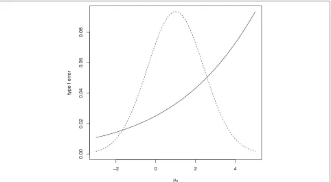
Figure4 shows the one-sided type I error rate for this design for a range ofμ0values with, in each case,μ1=μ0 so thatθ = 0. It can be seen that in this case although
the type I error rate is controlled forμ0 = 0, the type I error rate increases above the desired level forμ0>0. The figure also shows the prior distribution for μ0, showing that error rate inflation would occur for plausible values ofμ0.
Discussion
Our comparison has been restricted on the whole to group-sequential tests based on normally distributed test statistics. Although some exact or non-normal frequentist group-sequential test methods have been
proposed [27–29] the assumption of normality is
common in this setting. In Bayesian group-sequential tests it is more common to use non-normal
dis-tributions, with simulation methods being used
if necessary to calculate operating characteristics. The decision to focus on normally distributed test statistics was made so as to put Bayesian and frequen-tist designs in a similar setting, facilitate comparison and identify relationships, such as that between the Pocock test and the Bayesian test with a non-informative prior distribution, which might otherwise not be apparent. As can be seen from the binary data example above, where the Pocock test and the exact Bayesian test give identical stopping rules, in practice asymptotic normality can be a reasonable assumption.
Fig. 4Type I error rate for Bayesian test withK=5 andp1= · · · =p5=0.9884 for range of trueμ0values along with density (not to scale) for the
[image:11.595.59.541.438.703.2]We have considered stopping for a positive result only. In practice, with both frequentist and Bayesian group-sequential designs, it is often desirable to allow stopping when a lack of efficacy is clear, that is for futility. Futility stopping rules can be divided into those that are binding, when the rule is specified in advance and must be adhered to in order to maintain the required properties of the design, and those that are non-binding, where a more flex-ible approach can be taken. As stopping for futility cannot lead to a positive claim of efficacy, it can only decrease the type I error rate. Thus with a non-binding futility stopping rule, it is desirable to control the type I error rate even if no futility stopping occurs, that is in the case when the trial is only stopped for a positive result as considered above. The use of a binding futility stopping rule will change the operating characteristics of the group-sequential tests.
We have focussed on comparison of Bayesian and frequentist group-sequential designs for single-arm and comparative studies. These are just one type of adaptive design, which can include many other features includ-ing adaptive exploration of a dose-response relationship, adaptive randomisation, dropping of arms in multi-arm trials, incorporation of multiple endpoints and sample size reestimation. Frequentist methods that guarantee control of error rates are available for some of these problems such as sample size re-estimation [30] but in some other cases construction of decision rules for frequentist methods can be challenging. Bayesian methods can be accompanied by simulations to verify operating characteristics under a likely range of scenarios for a wide variety of adapta-tions for which rigorous proof of error rate control is not available.
Conclusions
Although Bayesian and frequentist group-sequential
approaches are based on fundamentally different
paradigms, in practice, when used for the analysis of a clinical trial, both provide an indication of the efficacy of an experimental treatment. This means that a com-parison of Bayesian and frequentist test can be helpful to understand the frequentist operating characteristics for Bayesian tests and the Bayesian model and prior distributional assumptions that could lead to a particular frequentist test. This has been our aim in this paper.
Focussing on a setting in which test statistics can be assumed to be normally distributed, we have shown that in comparative trials with independent prior distributions specified for treatment effects in different groups, stop-ping rules from Bayesian and frequentist group-sequential designs cannot generally correspond. In this case the Bayesian group-sequential design can then only control the type I error rate for specified values of the control group treatment effect. Conversely, in single-arm trials, or when a prior distribution is specified for the treatment
difference, stopping rules for Bayesian and frequentist group-sequential tests can be identical if full flexibility for both classes of designs is allowed, or can closely corre-spond for common choices of design parameters.
O’Brien and Fleming’s design was found to correspond closely to a Bayesian design with an exceptionally infor-mative negative prior, this prior leading to the very small probability of early stopping for this design. The fact that such a prior is unlikely to represent prior belief sug-gests that the use of this design might not be appropriate without very careful thought.
In a similar way, noting that the Bayesian design with a non-informative prior andp1= · · · = pK corresponds to a Pocock design suggests that this might also not be gen-erally appropriate given the criticism that this design gives too high a probability of early stopping [31]. This illus-trates the importance of appropriate choice of a prior dis-tribution, rather than the general use of a non-informative prior. Evaluation of the frequentist properties can be use-ful in understanding the influence of the prior distribution in a Bayesian group-sequential design in which the overall type I error rate is controlled.
Bayesian adaptive methods are often more bespoke than frequentist approaches, with simulations used to evalu-ate their performance not only for a range of treatment effect scenarios but also allowing for anticipated data patterns arising from, for example, delayed responses, multiple endpoints including early outcomes, or differ-ent recruitmdiffer-ent and drop-out rates. This can require more design work than the use of a more standard frequentist method but can be advantageous in that design choices and their consequences are considered carefully. It is recommended that if frequentist meth-ods are used, equal care should be taken over design choices and their properties explored, using simulations if necessary.
Appendix A: Comparison of posterior variances for comparative trials with single or independent prior distributions
Suppose we are in the two-group setting and have inde-pendent prior distributions withμj ∼ N μj0,Ij−01
,j =
0, 1 and that we have observation of Y¯jk with Y¯jk ∼
N(θ,Ik−1),j = 0, 1,k = 1,. . .,K, so that the posterior distribution forθis given by (10).
Considering only the single parameterθ, the posterior distribution is given by (10) withθ0 = μ10−μ00,I0−1 =
I00−1+I10−1andIk = I0−k1+I1−k1
−1 .
Let I[1]k and I[2]k denote the inverses of the posterior
variance for θ in the one-parameter and two-parameter
cases respectively. We will show thatI[1]k≤I[2]k.
rk = kr0andI1k = kr0I0k. Without loss of generality, we will takeI0k = 1 so thatI1k = kr0. We then have
I[1]k = I00/ 1+r−01
+ 1/1+(kr0)−1
and I[2]k = 1/(I00+1)−1+(r0I00+r0k)−1
.
LettingRkdenote the ratioI[1]k/I[2]kand differentiating this with respect tokyields
dRk
dk =
r0I00(a2k+bk+c)
(I00+1)(1+r0)(I00+k)2(kr0+1)2 .
witha= −(r0I00+2r0+1),b=2(r0−I00)andc=I00(r0+ 2)+1. Note that the derivative is defined for allk≥0 as
I00andr0are both positive. Setting the numerator to zero and solving the quadratic, we find thatRk has stationary points atk=1 and−(r0I00+2I00+1)/(r0I00+2r0+1). The second of these is negative asI00andr0are positive, so that the only stationary point withk≥0 is atk =1 whenRk =1
The second derivative ofRkwith respect tokatk = 1 is equal to−2r0I00(I00+1)−2(r0+1)−2, and so is neg-ative, confirming that the turning point is a maximum so thatRk ≤1, and henceI[1]k ≤I[2]k, as stated.
Appendix B: Type I error rate for Bayesian comparative trial with independent prior distributions
The requirement (5) that the error rate is controlled at levelαin the two-paramter case can be stated as
Pr(Pr(θ >0| ¯Y1k,Y¯0k)≥pksomek≤K;μ1=μ0)≤αfor allμ0.
(11)
We can rewrite the posterior distribuion (10) as θ |
¯
y1k,y¯0k ∼N Mk,I[2]−1k
withI[2]−1k =(I10+I1k)−1+(I00+
I0k)−1and
Mk= μ10
I10+ ¯y1kI1k
I10+I1k −
μ00I00+ ¯y0kI0k
I00+I0k
. (12)
The posterior probabilitypr(θ > 0 | ¯y1k,y¯0k)is thus equal to 1− −MkI[2]1/2k
. This exceeds pk whenever
Mk ≥ −−1(1−pk)I[2]−1/2k .
Hence in this case the stopping decision for the Bayesian sequential test depends on Y¯1k and Y¯0k via Mk and the frequentist operating characteristics for the Bayesian sequential test can be obtained from the joint distribution ofM1,. . .,MK.
It follows from (12) and (1) thatM1,. . .,MK are multi-variate normal with
E(Mk)= μ10
I10+μ1I1k
I10+I1k −
μ00I00+μ0I0k
I00+I0k .
Whenμ1=μ0, we have
E(Mk)= μ10
I10
I10+I1k −
μ00I00
I00+I0k +μ0
I1k
I10+I1k−
I0k
I00+I0k
.
If I1k
I10+I1k −
I0k
I00+I0k > 0, we haveE(Mk)→ ∞asμ0 → ∞, and if I1k
I10+I1k −
I0k
I00+I0k < 0, we haveE(Mk) → ∞as
μ0→ −∞. In neither of these cases, then, is it possible to satisfy (11) for all values ofμ0other than in the trival case withp1=1, when stopping is impossible.
Abbreviations
CDAI: Crohn’s disease activity index
Acknowledgements
The authors are grateful to an Editor and two referees for their comments on an earlier draft of the paper.
Authors’ contributions
NS conceived and undertook the research with feedback from all other authors. NS, ST, ER and SG discussed and commented on the manuscript. NS, ST, ER and SG read and approved the final manuscript.
Funding
NS, SG and EGR were supported by a Medical Research Council (MRC) Methodology Research Grant (Grant number: MR/N02828/1) during the conduct of this research. The funder had no role in the design of the study, collection, analysis and interpretation of data, or in writing the manuscript.
Availability of data and materials
Not applicable: no data or materials were used in this research.
Ethics approval and consent to participate
Not applicable: no patient data were used in this research.
Consent for publication
Not applicable: no patient data were used in this research.
Competing interests
The authors declare that they have no competing interests.
Author details
1Statistics and Epidemiology, Division of Health Sciences, Warwick Medical School, University of Warwick, Coventry, UK.2Department of Mathematics and Statistics, University of Reading, Reading, UK.3Cancer Research UK Clinical Trials Unit, Institute of Cancer and Genomic Sciences, University of Birmingham, Birmingham, UK.
Received: 20 September 2019 Accepted: 23 December 2019
References
1. Jennison C, Turnbull BW. Group Sequential Methods with Applications to Clinical Trials. Boca Raton: Chapman & Hall; 2000.
2. Berry SM, Carlin BP, Lee JJ, Müller P. Bayesian Adaptive Methods for Clinical Trials. Boca Raton: CRC Press; 2011.
3. Zhu H, Yu Q. A Bayesian sequential design using alpha spending function to control type I error. Stat Methods Med Res. 2017;26:2184–69. 4. Spiegelhalter DJ, Freedman LS, Parmar MKB. Bayesian approaches to
randomized trials. J R Stat Soc Ser A. 1994;157:357–416.
5. Ryan EG, Bruce J, Metcalfe AJ, Stallard N, Lamb SE, Viele K, Young D, Gates S. Using Bayesian adaptive designs to improve phase III trials: a respiratory care example. BMC Med Res Methodol. 2019;19:99. 6. Food and Drug Administration. Adaptive Designs for Clinical Trials of
Drugs and Biologics: Guidance for Industry. 2019.https://www.fda.gov/ media/78495/download. Accessed: 3 Jan 2020.
7. Hueber W, Sands BE, Lewitzky S, Vandemeulebroecke M, Reinisch W, Higgins PDR, Wehkamp J, Feagan BG, Yao MD, Karczewski M, Karczewski J, Pezous N, Bek S, Bruin G, Mellgard B, Berger C, Londei M, Bertolino AP, Tougas G, Travis SPL. Secukinumab, a human anti-IL-17A monoclonal antibody, for moderate to severe crohn’s disease: unexpected results of a randomised, double-blind placebo-controlled trial. Gut. 2012;61:1693–700.
9. Gerber F, Gsponer T. Package ‘gsbDesign’. 2016.http://CRAN.R-project. org/web/packages/gsbDesign/gsbDesign.pdf. Accessed: 3 Jan 2020. 10. Wilber DJ, Pappone C, Neuzil P, Paola AD, Marchlinski F, Natale A,
Macle L, Daoud EG, Calkins H, Hall B, Reddy V, Augello G, Reynolds MR, Vinekar C, Liu CY, Berry SM, Berry DA. Comparison of antiarrhythmic drug therapy and radiofrequency catheter ablation in patients with paroxysmal atrial fibrillation. J Am Med Assoc. 2010;303:333–40. 11. Emerson SS, Kittelson JM, Gillen DL. Bayesian evaluation of group
sequential clinical trial designs. Stat Med. 2007;26:1431–49. 12. Emerson SS, Kittelson JM, Gillen DL. Frequentist evaluation of group
sequential clinical trial designs. Stat Med. 2007;26:5047–80.
13. Campbell G. Similarities and differences of Bayesian designs and adaptive designs for medical devices: a regulatory view. Stat Biopharm Res. 2013;5: 356–68.
14. Shi H, Yin G. Control of type I error rates in Bayesian sequential designs. Bayesian Anal. 2018.https://doi.org/10.1214/18-ba1109.
15. Bernado JM, Smith AFM. Bayesian Theory. Chichester: Wiley; 2000. 16. Jennison C, Turnbull BW. Group sequential analysis incorporting
covariate information. J Am Stat Assoc. 1997;92:1330–41. 17. Saville BR, Connor JT, Ayers GD, Alvarez J. The utility of Bayesian
predictive probabilities for interim monitoring of clinical trials. Clin Trials. 2014;11:485–93.
18. Mujagic E, Zwimpfer T, Marti WR, Zwahlen M, Hoffmann H, Kindler C, Fux C, Misteli H, Iselin L, Lugli AK, Nebiker CA, von Holzen U, Vinzens F, von Strauss M, Reck S, Kraljevi´c M, Widmer AF, Oertli D, Rosenthal R, Weber WP. Evaluating the optimal timing of surgical antimicrobial prophylaxis: study protocol for a randomized controlled trial. Trials. 2014;15:188.
19. Pocock SJ. Group sequential methods in the design and analysis of clinical trials. Biometrika. 1977;64:191–9.
20. O’Brien PC, Fleming TR. A multiple testing procedure for clinical trials. Biometrics. 1979;35:549–56.
21. Genz A, Bretz F, Miwa T, Mi X, Leisch F, Scheipl F, Bornkamp B, Mæchler M, Hothorn T. Package ‘mvtnorm’. 2018.http://CRAN.R-project. org/web/packages/mvtnorm/mvtnorm.pdf. Accessed: 3 Jan 2020. 22. Slud EV, Wei LJ. Two-sample repeated significance tests based on the
modified Wilcoxon statistics. J Am Stat Assoc. 1982;77:862–8. 23. Lan KKG, DeMets DL. Discrete sequential boundaries for clinical trials.
Biometrika. 1983;70:659–63.
24. Proschan M, Lan KKG, Wittes JT. Statistical Monitoring of Clinical Trials: A Unified Approach. New York: Springer; 2006.
25. Kim K, DeMets DL. Design and analysis of group sequential tests based on the type I error spending rate function. Biometrika. 1987;74:149–54. 26. Anderson K. Package ‘gsDesign’. 2016.http://CRAN.R-project.org/web/
packages/gsDesign/gsDesign.pdf. Accessed: 3 Jan 2020.
27. Jennison C, Turnbull BW. Exact calculations for sequentialt,χ2andF tests. Biometrika. 1991;78:133–41.
28. Stallard N, Todd S. Exact sequential tests for single samples of discrete responses using spending functions. Stat Med. 2000;19:3051–64. 29. Stallard N, Rosenberger WF. Exact group-sequential designs for clinical
trials with randomized play-the-winner allocation. Stat Med. 2002;21: 467–80.
30. Cui L, Hung HMJ, Wang S-J. Modification of sample size in group sequential clinical trials. Biometrics. 1999;55:853–7.
31. Pocock S, White I. Trials stopped early: too good to be true? Lancet. 1999;353:943–4.
Publisher’s Note