Laser dimpling process parameters selection and optimization using surrogate driven process capability space

warwick.ac.uk/lib-publications

Ozkat, Erkan Caner, Franciosa, Pasquale and Ceglarek, Dariusz . (2017) Laser dimpling process parameters selection and optimization using surrogate-driven process capability space. Optics & Laser Technology, 93. pp. 149-164.

Permanent WRAP URL:

http://wrap.warwick.ac.uk/87875

Copyright and reuse:

The Warwick Research Archive Portal (WRAP) makes this work by researchers of the University of Warwick available open access under the following conditions. Copyright © and all moral rights to the version of the paper presented here belong to the individual author(s) and/or other copyright owners. To the extent reasonable and practicable the material made available in WRAP has been checked for eligibility before being made available.

Copies of full items can be used for personal research or study, educational, or not-for-profit purposes without prior permission or charge. Provided that the authors, title and full bibliographic details are credited, a hyperlink and/or URL is given for the original metadata page and the content is not changed in any way.

Publisher’s statement:

© 2017, Elsevier. Licensed under the Creative Commons Attribution-NonCommercial-NoDerivatives 4.0 International http://creativecommons.org/licenses/by-nc-nd/4.0/ A note on versions:

The version presented here may differ from the published version or, version of record, if you wish to cite this item you are advised to consult the publisher’s version. Please see the ‘permanent WRAP URL’ above for details on accessing the published version and note that access may require a subscription.

Laser dimpling process parameters selection and optimization using

surrogate-driven process capability space

Erkan Caner Ozkat* (a), Pasquale Franciosa(a)_{, Dariusz Ceglarek}(a)

(a) _{Warwick Manufacturing Group, University of Warwick, Gibbet Hill Rd., Coventry CV4 7AL, UK}

E – mail: [email protected], [email protected], [email protected]

Abstract

Remote laser welding technology offers opportunities for high production throughput at a

competitive cost. However, the remote laser welding process of zinc-coated sheet metal parts

in lap joint configuration poses a challenge due to the difference between the melting

temperature of the steel (∼1500 C) and the vaporizing temperature of the zinc (~907 C). In fact, the zinc layer at the faying surface is vaporized and the vapour might be trapped within

the melting pool leading to weld defects. Various solutions have been proposed to overcome

this problem over the years. Among them, laser dimpling has been adopted by manufacturers

because of its flexibility and effectiveness along with its cost advantages. In essence, the dimple works as a spacer between the two sheets in lap joint and allows the zinc vapour escape during

welding process, thereby preventing weld defects. However, there is a lack of comprehensive

characterization of dimpling process for effective implementation in real manufacturing system

taking into consideration inherent changes in variability of process parameters. This paper

introduces a methodology to develop (i) surrogate model for dimpling process characterization

considering multiple–inputs (i.e. key control characteristics) and multiple–outputs (i.e. key

performance indicators) system by conducting physical experimentation and using multivariate

adaptive regression splines; (ii) process capability space (Cp–Space) based on the developed

surrogate model that allows the estimation of a desired process fallout rate in the case of

violation of process requirements in the presence of stochastic variation; and, (iii) selection and

optimization of the process parameters based on the process capability space. The proposed

methodology provides a unique capability to: (i) simulate the effect of process variation as

generated by manufacturing process; (ii) model quality requirements with multiple and coupled

quality requirements; and (iii) optimize process parameters under competing quality

requirements such as maximizing the dimple height while minimizing the dimple lower surface

area.

Keywords Laser dimpling · Zinc coated steel · Surrogate modelling · Design of experiment ·

Nomenclature

𝐷_𝐻 Dimple height

𝐷𝑈 Dimple upper surface area 𝐷_𝐿 Dimple lower surface area

𝑆_𝑠 Scanning speed

𝛼 Incidence angle

𝐹𝑂 Focal offset

𝐿_𝑇 Laser track

𝐾𝐶𝐶𝑠 Key Control Characteristics 𝐾𝑃𝐼𝑠 Key Performance Indicators

𝑁_𝑖 Number of KCCs

𝑁_𝑗 Number of KPIs

𝑁_𝑘 Number of experimental configurations 𝑁_𝑙 Number of experiment replications

𝑑 Number of dependent KPIs

𝑁_𝑠(𝑘) Number of KPIs in the 𝑘𝑡ℎ experimental configuration 𝐾𝐶𝐶_𝑖(𝑘) 𝑖𝑡ℎ KCC value in the 𝑘𝑡ℎ experimental configuration

𝐾𝑃𝐼_𝑗(𝑘,𝑙) 𝑗𝑡ℎ KPI value in the 𝑘𝑡ℎ experimental configuration at the 𝑙𝑡ℎ replication 𝜇_𝐾𝑃𝐼

𝑗(𝑘) Mean value of the 𝑗

𝑡ℎ _{KPI in the 𝑘}𝑡ℎ _{experimental configuration}

𝜎_𝐾𝑃𝐼

𝑗(𝑘) Standard deviation of the 𝑗

𝑡ℎ _{KPI in the 𝑘}𝑡ℎ _{experimental configuration}

𝜇̂_{𝐾𝑃𝐼𝑗} Estimated mean value of the 𝑗𝑡ℎ KPI

_𝐾𝑃𝐼

𝑗(𝑘) Success rate of the 𝑗

𝑡ℎ _{KPI in the 𝑘}𝑡ℎ _{experimental configuration}

_𝐾𝑃𝐼

1(𝑘)⋯𝐾𝑃𝐼𝑑(𝑘) Success rate of the dependent KPIs in the 𝑘

𝑡ℎ _{experimental configuration}



̂

𝐾𝑃𝐼𝑗 Estimated success rate of the 𝑗

𝑡ℎ _KPI

̂

𝐾𝑃𝐼1⋯𝐾𝑃𝐼𝑑 Estimated success rate of dependent KPIs

𝐹_{𝜇𝐾𝑃𝐼𝑗} Deterministic surrogate model of the 𝑗𝑡ℎ KPI 𝐹_

𝐾𝑃𝐼𝑗 Stochastic surrogate model of the 𝑗

𝑡ℎ _KPI 𝐹_

𝐾𝑃𝐼1⋯𝐾𝑃𝐼𝑑 Stochastic surrogate model of dependent KPIs

𝑃𝐷𝐹 Probability density function

𝑆𝑅 Success rate

𝛽 Minimal desirable success rate

𝐿𝐿 Lower limit

𝑈𝐿 Upper limit

KCC − space Process parameter space 𝐂_𝐩− 𝐬𝐩𝐚𝐜𝐞 Process capability space

𝐃𝐂𝐩𝐣 – 𝐒𝐩𝐚𝐜𝐞 Deterministic process capability space of 𝑗𝑡ℎ KPI

𝐒𝐂_𝐩𝐣 – 𝐒𝐩𝐚𝐜𝐞 Stochastic process capability space of 𝑗𝑡ℎ KPI 𝐃𝐂_𝐩 – 𝐒𝐩𝐚𝐜𝐞 Deterministic process capability space

1

1. Introduction

Thin zinc coated steel sheets are widely used in the automotive industry due to its high

corrosion resistance, especially in body-in-white and closure panels [1,2]. With the

advancement of the laser technology, laser welding has been gradually replacing traditional

5

welding methods since it offers cheaper and faster manufacturing process as well as better

mechanical and aesthetic joint quality [3–5]. Despite such benefits, it is nonetheless challenging

to achieve high quality joint in lap joint configuration of zinc coated steel since the boiling point

of zinc (~907 C) is significantly lower than the melting point of steel (~1500 C), resulting in

highly pressurized zinc vapour on the faying surfaces during the welding process. Left

10

unaddressed, such zinc vapour can easily be trapped inside the molten pool which can lead to

welding defects such as porosity, spatter, burn-through, and severe undercuts [6,7].

Over the past few years, significant amount of researches have been conducted to prevent the molten pool from being destroyed by the zinc vapour and several solutions have been proposed which can be classified as:

15

 Ventilation – This method is based on degasification of zinc vapour from the medium without

causing any weld defects either by enlarging molten pool [8,9]; stabilizing the keyhole by

employing shielding gas [10,11]; creating pre-drilled ventilation channels [12]; applying

appropriate spacers at the faying surfaces [13–15]; or adopting a suction method to remove

20

the vapour [16];

 Inserting a thin metal foil – This involves adding another material (e.g. Al & Cu) into the

faying surface which absorbs zinc vapour or reacts with zinc vapour in such a way that a

liquid alloy with a high boiling point is formed [17,18];

 Tandem beams – This approach employs a dual laser beam or a secondary heat source. The

25

first beam applies pre-heating which vaporizes zinc coating and second beam performs actual

welding [19–21];

 Controlling keyhole oscillation – The molten pool shape can be controlled based on the pulsed wave mode of laser beam so that more stable keyhole oscillation can be achieved,

allowing the zinc vapour to escape during the keyhole closure [22,23]

30

 Surf-sculpt – This method creates surface features from the base metal by repeated movement

of the low power on-focus laser beam in a short distance. These features increase surface

area of the material and can be utilized as a spacer between the faying surface in lap joint

2

All of the above solutions have been shown to produce satisfactory welds in lap joint

35

configuration. However, they do have number of disadvantages due to: (i) challenges in

development of system automation for robotic joining process (see inserting a thin metal foil

solution); (ii) increased system complexity (see ventilation and tandem beam solutions) due to

the need for installation of additional equipment which increases processing cost as well; and,

(iii) increased cycle time (see tandem beam, controlling keyhole oscillation and surf-sculpt

40

solutions) due to lower processing speed.

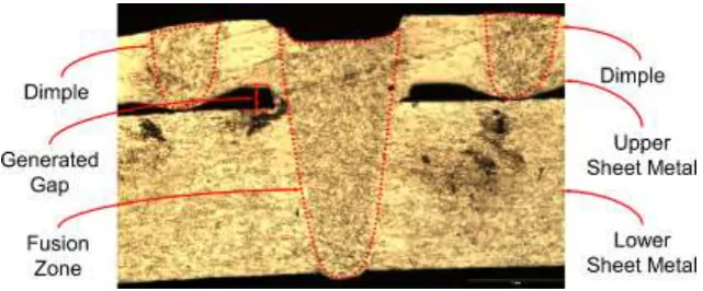
A promising technique for mitigation of zinc vapour is “laser dimpling” which makes a

dimple on the faying surface of the upper sheet metal by rapid and single movement of the laser beam. Hence, the zinc vapour is vented out through the generated gap between the faying

surfaces which is illustrated in Fig. 1. The laser dimpling process has been used by the

45

automotive industry as it does not require any additional equipment and can be performed using

the same laser source and fixture adopted for welding [26,27]. Furthermore, it is not restricted

by the shape and curvature of the workpiece and weld location.

50

Fig. 1. Micro-section of laser welded joint with laser dimpling technique

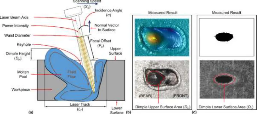
The physical principle behind laser dimpling process can be explained by the “humping

effect” which is influenced by the heat and mass transfer in the molten pool. In general, humps

occur periodically along the weld bead which deteriorate the homogeneity of molten pool. In

55

laser welding process, when the beam hits the workpiece, it creates a deep narrow cavity, known

as keyhole. While laser beam is moving, the liquid material at the bottom of the keyhole flows

upwards to the rear of the molten pool and generates a backward trail of a thin jet due to the

surface tension on the keyhole walls. The solidification of this jet on the surface forms the hump

at the rear and leading to a valley of cavity at the front which is given in Fig. 2. There has been

60

significant research which look at the humping effect as a negative phenomenon during joining

3

the hump [28–32]. However, the “humping effect” can be beneficially utilized by laser dimpling

process to create the required gap in lap welding of zinc coated steels.

65

Fig. 2. (a) Illustration of humping effect during a dimpling process (b) dimple upper surface (c) dimple

lower surface

According to Gu [26,27], humping effect was used to generate dimple for laser welding

70

process first, by studying the influence of a single parameter, focal offset, on the dimple height.

Then, they used this information to generate dimples at different scanning speed and incidence

angle, while other parameters such as focal offset were kept constant. Results indicated that

dimple height monotonically decreased with increasing both scanning speed and incidence

angle; whereas, the dimple height firstly, increased and then decreased whilst increasing the

75

focal offset. In a more recent study conducted by Colombo and Previtali [33] applied univariate

linear regression model to determine influence of scanning speed on the dimple height keeping

constant laser power, focal offset, and laser track. They found that linear energy, which is the

amount of the energy supplied per unit time, was the primary factor affecting the dimple height.

However, this study has limitation as authors considered only the influence of a single process

80

parameter without exploring other important process parameters and their interactions.

The existing literature has focussed mainly on single–input (i.e. scanning speed) and single–

output (i.e. dimple height) scenario which is necessary but not sufficient to give a complete

characterisation of the dimpling process. Furthermore, the laser material processes are

characterized as multiple–inputs and multiple–outputs (MIMO) system with non-linear

85

functional relationship [34–36].

Thus, it is important to take into consideration MIMO–based scenario for dimpling process.

4

parameters for a dimpling process: scanning speed (SS), focal offset (FO), incidence angle (𝛼);

and, laser track (LT) as well as the following three key performance indicators (KPIs) to be 90

addressed as multiple–outputs parameters: dimple height (DH), dimple upper surface area (DU);

and, dimple lower surface area (DL).

Another limitation associated with the current literature is the lack of modelling variation in

the dimpling process. The current models are developed under the assumption of ideal process

performance neglecting process variation. As a result of lack of understanding process

95

variation, the measurement of selected KPI (e.g. dimple height) for given process parameters

might violate the given allowance limits and it will lead to erroneous process parameters

selection. However, no comprehensive research work has been reported in the laser dimpling

process that considers MIMO–based scenario with process variation.

This study is, therefore, focused on development of: (i) surrogate model for dimpling

100

process characterization considering multiple–inputs and multiple–outputs (MIMO) system by

conducting physical experimentation and using multivariate adaptive regression splines; (ii)

process capability space (Cp–space) for deterministic and stochastic cases based on the

developed surrogate models; and (iii) optimization of the process parameters based on the

process capability space.

105

The methodology is developed by introducing the concepts of deterministic and stochastic

process capability spaces. The deterministic Cp–space is a measure of the dimpling process

capability to satisfy simultaneously all the KPIs allowance limits requirements. Whereas, the

stochastic Cp–space is the estimation of process fallout rate which is the probability of making

a dimple which satisfies simultaneously all the KPIs limits requirements. The stochastic Cp–

110

space is then used to develop robust dimpling process by identifying process parameters which

are less sensitive to the variation in process.

2. Problem Formulation 115

2.1. Definition of key control characteristics (KCCs) and key performance indicators (KPIs)

The quality performance of a dimple is evaluated by multiple–outputs called in this paper

as Key Performance Indicators (KPIs), which are delivered by process parameters (multiple–

inputs), named in this paper as Key Control Characteristics (KCCs). As shown in Fig. 2, the

120

5  Scanning speed (SS) – The travelling speed of the laser beam along the upper surface of the

workpiece;

 Focal offset (FO) – The distance along the beam axis between the focal point and the 125

interaction of beam and upper surface of the workpiece;

 Incidence angle (α) – The angle along the beam movement between the beam axis and the

normal vector to the upper surface of the workpiece;

 Laser track (LT) – The linear distance of the beam movement to make a dimple which is

parallel to the upper surface of the workpiece.

130

We observe that the aforementioned KCCs affect not only the selected dimpling process

KPIs, but also KPIs of other downstream processes. For example, scanning speed and laser track

can affect process cycle time and fixture clamp layout design [37]. Moreover, focal offset and

incidence angle can be related to not only dimple height or dimple upper surface area but also

135

they can affect detailed 3D fixture design includes the beam visibility, accessibility and offline

programming of the robotic scanner head. This is caused by the fact that the robotic system used

to make dimples needs to gain access to the workpiece with no collision between the

workpiece/fixture and the laser beam. These examples illustrate the importance analysing

dimpling process as MIMO–based system and also to develop methodology which can be

140

expanded to include additional KPIs as required by downstream processes.

Let us define that four KCCs (SS, FO, α, LT) are gathered as in Eq. (1), where 𝑖 and 𝑘 represent

index of KCC and experimental configuration





KCC ; whereas, 𝑁_𝑖 and 𝑁_𝑘 are the total

number of KCCs and experimental configurations, respectively.

145

   

 

   

1 1

1

1

i

k k

i N

k i

N N

N

KCC KCC

KCC

KCC KCC

 

 

 



 

 

 

KCCs (1)

The following KPIs are proposed to measure the functionality, strength and aesthetic quality

requirements of the dimple which are illustrated in Fig. 2.

150

 Dimple Height (DH) – This KPI is needed to evaluate the required and predetermined gap

between over lapped sheet metal parts which is the main functional objective of a dimple. It

is reported in the literature that to make joints with satisfactory quality in laser lap welding

6  Dimple upper surface area (DU) – This KPI assesses (i) strength of the dimple to prevent 155

excessive deformation of the dimple height under compression of clamping force applied during welding process; and, (ii) uncertainty as measured by difference between dimple

height and the required gap between the faying surfaces during consecutive welding process

and caused by geometric surface defects such as roughness, scratches, lines and etc. In

essence, the larger dimple upper surface area generates stronger and higher dimples but it

160

creates unwanted surface feature such as dark spots in the lower surface of the workpiece.

According to initial screening experiments, we propose dimple upper surface area should

be in the range of [1.0, 5.0] mm2 in order to generate sufficient gap between faying surfaces

to achieve satisfactory joint in laser lap welding.

 Dimple lower surface area (DL) – The dark spot appeared in the dimple lower surface is an 165

aesthetic quality requirement which is an unwanted feature in Class-A surfaces in the

automotive industry [38]. Thus, the objective is to determine dimple lower surface area

which minimizes dimple height variation under compression clamping force in lap joint.

According to initial screening experiments, we propose dimple lower surface area should

be in the range of [0, 1.5] mm2.

170

Let us define three KPIs (DH, DUand DL), as shown in Eq. (2), where 𝑗, 𝑘 and 𝑙 represent

index of KPI, experimental configuration number and its replication





KPI ; whereas, 𝑁_𝑗, 𝑁_𝑘

and 𝑁_𝑙 are the total number of KPIs, experimental configurations and replicates, respectively.

175





k k l

j

N

j j

k l j

N N N

j j N KPI KPI KPI KPI KPI                j j KPIs KPI KPI (2)

The aforementioned three KPIs are selected as the primary indicators used in this paper to

evaluated dimpling process. Additionally, the paper defines lower limits (LL) and upper limits

(UL) for each KCC and KPI, which are given in Tables 1 and 2, respectively.

180

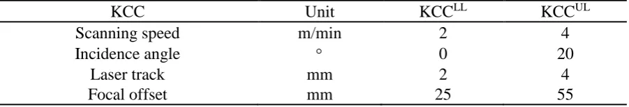
Table 1 KCCs and their corresponding allowance limits

KCC Unit KCCLL KCCUL

Scanning speed m/min 2 4

Incidence angle  0 20

Laser track mm 2 4

7

The lower and upper limits of all KCCs have been defined by taking into account

technological constraints such as maximum scanning speed of the laser beam, minimum laser

power intensity on the upper surface of the workpiece to create a dimple. These limits were

185

determined by conducting initial dimpling and welding experiments, results of which are not

reported in the paper. The set of all possible KCCs within the allowance limits defines the

process parameters space (KCC–space). On the other hand, the lower and upper allowance

limits of all KPIs are determined based on aforementioned quality requirements.

190

Table 2 KPIs and their corresponding allowance limits

KPI Unit KPILL KPIUL

Dimple height mm 0.1 0.3

Dimple upper surface area mm2 _{1.0 5.0}

Dimple lower surface area mm2 0.0 1.5

2.2. Formulation of surrogate modelling for the dimpling process characterization

The proposed modelling approach addresses two key limitations of the currently available

195

models for dimpling process characterization as discussed in the introduction section by taking

into consideration; (i) approximation of a comprehensive multivariate relations between

multiple– inputs (KCCs) and multiple–outputs (KPIs) of the dimpling process, and (ii) process

variation over the KCC–space which can be either homoscedasticity (all KPIs across the KCC–

space have the same variance) or heteroscedasticity (variability of a KPI is unequal across the

200

KCC–space). The process capability space (Cp–space) is presented to address both limitations

by defining a set of KPIs comprehensively evaluate dimpling process and identifying process

parameters inside the KCC–space that satisfy the given quality requirements.

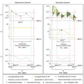
Two different scenarios are considered: deterministic and stochastic. In the deterministic

scenario, one or many measurements of the KPIs are conducted. Then, the mean values are

205

calculated to compute deterministic surrogate model which estimates the KPI values over the

KCC–space. A success rate (binary function) is therefore calculated which determines whether

the estimated value is within its lower and upper allowance limits for a given KPI. In case of

success, the given process parameters (KCCs) are said to be feasible. However, this modelling

approach has its own limitations. Indeed, due the stochastic nature of the KPI measurements,

210

some individual measurements might violate the limits contrary to its estimated value which

does not and vice-versa as highlighted in Fig. 3a.

Thus, stochastic scenario is proposed to take into account the mean and variance to calculate

8

variation can be represented as in the form of the success rate function. Initially, the probability

215

density function is developed either normal or non-normal distribution, using the measured

KPI values. Afterwards, the SR value is calculated which is the probability value of satisfying

the allowance limits as illustrated shaded regions in Fig. 3a. Finally, stochastic surrogate model

(non-binary function) is developed to calculate the SR values over the KCC–space to determine

the feasible KCCs for achieving given success rate () as highlighted in Fig. 3b

220

Furthermore, the success rate is also referred as (1 – process fallout rate) in the

manufacturing terminology and note is made that the higher success rate is the lower the process fallout rate. Moreover, the allowance limits for KCCs are determined by the equipment

capability; whereas, the specification limits for KCCs are determined to satisfy the allowance

limits for KPIs and the natural specification limits are determined to satisfy desirable success

225

rate, which are illustrated in Fig. 3c.

Fig. 3. Conceptual representation deterministic and stochastic scenarios; (a)Experimental results (b)

Success rate models (c) Tolerance limits 230

The observed KPIs might not be independent each other and their joint relationship becomes

important to define the PDF function. Therefore, the Pearson correlation coefficient test has

9 235

 

_

_

cov ,

, 1, ,

mn m n Nj

      m n m n KPI KPI KPI KPI (3)

The correlation result

 

between -1 and +1. Even though correlation and dependency are statistically different terms, if

KPIs are linearly correlated, it can be deduced that they are dependent each other. As a result,

240

the dependence among KPIs changes the form of the PDF function. The mean value of the 𝑘𝑡ℎ

experimental configuration of the jth _{KPI is defined in Eq. (4), where}  k s

N is the sample size in

the 𝑘𝑡ℎ experimental configuration.

  _{ }  

 

 1    

, 1 T 1 , , , , k s k j k Nk

j j j

N k l j k KPI l s

KPI KPI KPI

KPI N          _ _



The PDF function that describes the simultaneous behaviour of the dependent KPIs which

is called as “joint probability density function” is given in Eq. (5).

KPI KPI d k

PDF e        _  _  _  _      

d k d k

KPI_d KPI_d

KPI μ KPI μ

(5)

250

where d is the number of the dependent KPIs and it will equal to the number of KPIs (𝑁_𝑗),

if all KPIs are dependent to each other. The symmetric covariance matrix in the 𝑘𝑡ℎ

experimental configuration is given as _ k

. On the other hand, The PDF function is represented

as function of mean value

 

KPI

 and standard deviation

 

KPI

 for univariate independent

255

KPI, which is given in Eq. (6).

        2 1 2 1 2 j k KPI j k KPI j k j k j KPI KPI KPI PDF e             

 (6)

The Shapiro–Wilk normality test, which provides better results that other normality tests for

260

small sample size [39], is applied to assess the normality assumption for each experimental

10

number of replication is quite small to directly calculate the standard deviation. Therefore, it is

formulated using the range statistics and corrective coefficient (d2) constant.

The success rate is calculated as a probabilistic approach that is the area under the PDF

265

function. The probability is determined by the integral of the PDF over the given allowance

limits, and it is formulated in Eq. (7) for dependent KPIs; whereas, in Eq. (8) for each

independent KPI.            





1 , , 1 1, ,

UL UL

d

k k

k k _d

KPI KPI_{d LL LL}

d

KPI KPI

k k k k

d d K

KPI KPI KPI KPI

PDF KPI KPI dKPI dKPI k N

 

_

_

270

   





UL j

k LL k

j j j

KPI _{k k}

j j J K

KPI KPI PDFKPI KPI dKPI j d N k N

 

_

The general forms of deterministic and stochastic surrogate models for estimating KPI value

and the success rate for dependent and independent KPIs are given in Eqs. (9) to (11),

respectively.

275









ˆ , , 1, ,

j i

KPI KCC KCCN j Nj

   

KPIj μ

F (9)





1 1

ˆ _{, ,}

d i

KPI KPI KCC KCCN

 

KPI1 KPId ξ

F (10)









ˆ _{, , 1, ,}

j i

KPI KCC KCCN j d Nj

    

KPIj

ξ

F (11)

280

2.3. Formulation of deterministic and stochastic process capability space

A sub-set of KCC–space is the process capability space (Cp–space), which envelops all the

feasible KCCs satisfying the KPIs allowance limits. For the 𝑗𝑡ℎ KPI, deterministic process

capability space





p

DC - Space is expressed in Eq. (12).

285













1

, , 1

, , 1, ,

0

i i

LL UL

j N j

N j

if KPI KCC KCC KPI

KCC KCC j N

otherwise         KPIj j μ p F

DC - Space (12)

The stochastic process capability spaces are defined in Eqs. (13) & (14) for dependent and

independent KPIs, respectively.

290









1

ˆ _{, , 1}

, , 0 i d i N KPI KPI N

if KCC KCC

KCC KCC otherwise    _{ }    

KPI1 KPId KPI1 KPId

ξ p

F

SC - Space (13)









1

ˆ _{, , 1}

, , 1, ,

0 i j i N KPI N J

if KCC KCC

KCC KCC j d N

otherwise    _{ }       KPIj j ξ p F

11

where 𝛽 is the minimal desirable success rate. The identification of the final deterministic

295

and stochastic process capability spaces is done by aggregation individual deterministic and

stochastic process capability spaces and obtained from Eq. (15) and Eq. (16), respectively.

1 J j N j  p p

DC - Space DC - Space (15)

1

J

j

N

j d 





KPI1 KPId

p p p

SC - Space = SC - Space SC - Space. (16)

300

It is noteworthy that 𝑑 is the number of the dependent KPIs which is determined according to the Pearson correlation coefficient test. The final stochastic process capability space is

obtained by the probability theory which is a product of the independent and dependent

stochastic process capability spaces. If the all KPIs are dependent, final stochastic process

305

capability is only computed from the dependent stochastic process capability space.

2.4. Process parameter optimization using calculated surrogate models

The aim of this study is to identify optimum KCCs which maximize KPI (evaluated by

310

deterministic surrogate model) and the probability of satisfying the allowance limits of that KPI

(evaluated by stochastic surrogate model) at the same time. Therefore, the multi–objective

optimization problem can be formally stated in Eq. (17).





















1

1 1 1

maximize F , , , F , , , F , ,

1, , subject to

ˆ 1, ,

KPIj i KPIj i KPI KPId i

j

N N N

LL UL

i i i i

LL UL

j _KPI j j

KCC KCC KCC KCC KCC KCC KCC KCC KCC i N

KPI KPI j N

            (17) 315

3. Generation of the deterministic and the stochastic surrogate models

3.1 Materials

320

The material used in this study was DX54D hot dip galvanized (GI) steels with nominal zinc

coating thicknesses of 20 μm. The chemical composition and mechanical properties of this

steel are given in Tables 3 and 4, respectively.

Table 3 Chemical composition DX54D steel (wt %)

325

Material Elements (wt %)

C Si Mn P S Ti

12

Two series of experiments were carried out. The first series served to characterise the

dimpling process and develop the deterministic and stochastic process capability spaces;

dimples were generated on the top surface of zinc coated sheet metal with a thickness of 0.75

mm. The second series was used to validate the calculated optimum KCCs based on the process

330

capability spaces by confirmation experiments which were carried out on coupon experiments.

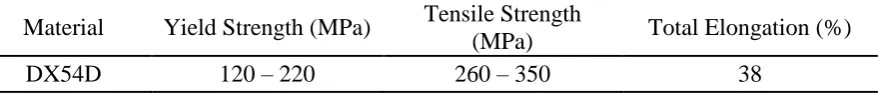
Table 4 Mechanical properties of steel DX54D

Material Yield Strength (MPa) Tensile Strength

(MPa) Total Elongation (%)

DX54D 120 – 220 260 – 350 38

335

3.2 Experimental setup

Dimpling experiments were carried out using IPG Photonics YLR-4000 laser source with a

nominal power of 3 kW at a wavelength of 1064 nm. The laser beam was delivered using an optical fiber of core diameter of 50 μm, projecting the laser beam to a spot of 900 μm diameter.

340

The laser source generates a multi-mode beam with an M2 of 31.4 (measured by Primes Focus

meter) at a central wavelength of 1064 nm. Neither shielding nor backing gases were used

during the experiments.

Figure 4 shows the experimental setup for beam quality measurement, laser dimpling and

remote welding systems. The laser beam is delivered by COMAU SmartLaser robotic system

345

which is a dedicated system for remote laser welding/dimpling and consists of 4 axes with

dynamics and kinematics of a standard industrial robot with an optical system able to deflect

the focused beam with high dynamics. The system specifications are given in Table 5.

350

Fig. 4. Overview of the experimental setup (a) Beam quality measurement (b) Laser Dimpling setup

13

Table 5 Laser focusing and repositioning module (SmartLaser)

Characteristic Feature Unit Specification

Collimating length mm 50

Max focal length mm ~1200

Measured spot size m 900

Working area mm 700 × 450 × 400 Working distance mm 𝑚𝑖𝑛 894 𝑚𝑎𝑥 1216

355

3D optical surface profilometer (Bruker, Contour GT) was used to measure dimple height

(DH) and dimple upper spot area (DU). The top surface of the zinc coated steel was scanned at

speed 5m/s with a vertical resolution of ~10 nm on a rectangle region 4.5 x 6.5 mm. Thus,

there are some gaps in the obtained data. The raw data obtained from the optical profilometer

was filtered and then reconstructed in 3D which was meshing of the scanned surface area using

360

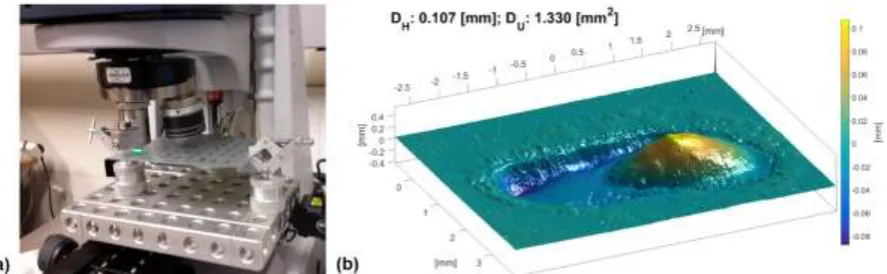
“Laplacian smoothing filter”. The experimental setup for profilometer and an example of

scanning result with corresponding process parametersare shown in Fig. 5.

Fig. 5. (a) Experimental setup for profilometer (b) An example of 3D reconstruction. Process

365

parameters: SS: 2 m/min, FO: 35 mm, : 20, LT: 4 mm

On the other hand, dimple lower surface area (DL) was computed by image segmentation

method using MatLab®. Each image is captured with high resolution camera (3264×2448

pixels), with focal axis perpendicular to the surface of the workpiece to avoid image distortion.

370

Initially, the number of pixel is calculated in 10 mm straight line to obtain scale from pixel

length to millimetre; and then, the image was converted into 256 grey levels. After removing

the background from the original image, it was binarized (black and white image). The number

of black pixels inside the binarized image gives the area in pixel unit. This is converted into

millimetre square using the obtain scale to get the corresponding lower surface area (DL). As 375

14

Fig. 6. Measurement of the dimple lower surface area (a) Grabbed image with scale bar. (b) Dimple

lower surface area (DL) for experiment configuration 19 with 5 replications. Process parameters: SS: 2 380

m/min, FO: 25 mm, : 10, LT: 4 mm

3.3 Design of Experiments

Several methods are available for the design of experiments to establish the relationship

385

between input and output variables, which include, among others, single-factor by single-factor

approach, factorial or fractional factorial approaches, Box-Behnken, Doehlet or Taguchi

experimental designs. Even though the full factorial design requires larger number of

experimental configurations than others alternative techniques, it allows to spread out design

point uniformly to obtain complete information on an unknown design function with a limited

390

sample size for capturing both main factors and interactions. Therefore, we adopted a full

factorial design approach with 4 – factor and 3 – level requires 81 experimental configurations

(Nk) with five replicates resulting 405 experimental runs. The design of experiment table was

created in randomize order and it was distributed into 9 batches of sheet metal plates (130 ×

110 mm). Thus, each plate had equal number of dimples and dimpling experiments were

395

conducted according to the created DoE table. However, this equal division did not guarantee

that each replicate was conducted in different metal plates. Due to the expected non-linear and

stochastic nature of the dimpling process, we selected 3 levels for each KCC and the selected

experimental levels were shown in Table 6.

400

Table 6 Key control characteristics and corresponding levels

KCC Unit Level [1] Level [2] Level [3]

Scanning Speed m/min 2.0 3.0 4.0

Incidence Angle  0.0 10.0 20.0

Focal Offset mm 25.0 35.0 55.0

15

Replication is conducted to detect the variation of system. Note is made that the more

number of replications is the more accurate estimation of variation within the system. We

selected 5 replications because they represent the right balance between expected model

405

accuracy and time needed to perform experiments and collect data (one single dimple

experiment, including laser processing, measurement and data collection, took about 2 hours).

The paper is intended to provide a general methodological approach, whose accuracy may be

enhanced whenever more replications are made available.

410

3.4 Developing of Surrogate Models

The first objective of this work is to compute a surrogate model capable of analytically

formulate relationships between multiple–inputs (KCCs) and multiple–outputs (KPI values and

success rates). This study applied multivariable adaptive regression spline (MARS) method

415

developed by Friedman [40]. The MARS method is a non-linear and non-parametric regression

that is able to model complex non-linear relationship among input variables by developing

regression models locally rather than globally by the dividing the parameter space into several

pieces and then performing piecewise fitting in each piece. Furthermore, it does not require

larger number of training data sets and long training process compared to other methods such

420

as neural networks, support vector machines [41].

The piecewise fitting is more appropriate for obtained data in dimpling experiments which

are actual measurements and calculated success rates. The behaviour of the obtained data in

one region inside the KCC–space cannot be easily correlated to its behaviour in other region

caused by a sudden change which reduces the goodness of the regression. For instance, high

425

success rate can be achieved in one experimental configuration but low success rate might be

obtained in the next experimental configuration. This sudden change can be handle by using

piecewise fitting methods.

The MARS models was developed using ARESLab© [42], a dedicated MatLab toolbox. The

parameters used for developing the surrogate models were; (i) the maximum number of basis

430

functions that included the intercept terms was set as 101. These functions were necessary to

build the model in the forward building phase; (ii) the maximum degree of interactions between

KCCs was set as 4; (iii) piecewise cubic type was chosen; (iv) the least important basis

functions and high-order interactions were eliminated by feature selection and Generalized

Cross-Validation (GCV) score in the backward elimination phase and set as 3; and, (v) k-fold

435

16

4. Development of the deterministic and the stochastic process capability spaces

The second objective of this work is to develop deterministic and stochastic process

capability spaces. A probabilistic approach was used to developed the stochastic capability

440

space. In some problems, the measured KPIs might be dependent each other and their

simultaneous behaviour defines the probability space. Therefore, the Pearson correlation

coefficient test was initially conducted to determine the number of the dependent KPIs (d). As

a consequence, a stochastic surrogate model and a stochastic process capability space were

computed for the dependent KPIs; whereas, different stochastic surrogate models and

445

stochastics process capability spaces were computed for each independent KPIs.

The Dixon’s Q test was employed for identification of outliers for each experimental

configuration and KPIs since it was designed for small sample size and assumed normal

distribution [43]. When an outlier detected in one of the dependent KPI, the corresponding

values in other KPIs were also considered as outlier even if the passed were not identified as

450

outliers. The procedure flow for computing final deterministic and stochastic process capability

spaces are summarized in Table 7.

Table 7 The procedure flow for computing process capability spaces

Step The methodology for computing final process capability spaces 1 Gather measurements for each KPI using Eq. (2)

2 Define number of dependent KPIs using Eq. (3)

3.1 Calculate outliers for each experimental configuration of each KPI using The Dixon’s Q test 3.2 Update the number of sample size for each experimental configuration

4.1 Calculate mean for each experimental configuration for each KPI using Eq. (4) 4.2 Calculate standard deviation for each experimental configuration for each KPI

 

 









 1    





. .

2

T

max min

, , , , 1, ,

k j

k Nk

j j j

k l k l

j j

KPI

j KPI KPI KPI

KPI KPI d j N          _{ }     j KPI

5.1 Calculate PDF for each experimental configuration for dependent KPIs using Eq. (5) 5.2 Calculate PDF for each experimental configuration for each independent KPI using Eq. (6) 6.1 Calculate SR for each experimental configuration for dependent KPIs using Eq. (7)

6.2 Calculate SR for each experimental configuration for each independent KPI using Eq. (8) 7.1 Calculate deterministic surrogate model for each KPI using Eq. (9)

7.2 Calculate stochastic surrogate model for dependent KPIs using Eq. (10) 7.3 Calculate stochastic surrogate model for each independent KPI using Eq. (11) 8.1 Calculate deterministic process capability space for each KPI using Eq. (12) 8.2 Calculate stochastic process capability space for dependent KPIs using Eq. (13) 8.3 Calculate stochastic process capability space for each independent KPI using Eq. (14) 9.1 Calculate final deterministic process capability over KCC–space using Eq. (15) 9.2 Calculate final stochastic process capability over KCC–space using Eq. (16) 455

17

The last objective of this work is optimization of the process parameters based on the

deterministic and stochastic process capability spaces. Both deterministic and stochastic Cp–

spaces provide necessary models for selection KCCs to optimize the KPIs using various

strategies reflecting the engineering needs of the dimpling process. In general, the optimisation

460

entails two competing objectives; (i) to obtain maximum KPI value; and, (ii) to maximize the

probability of satisfying the allowance limits of selected KPI. It is important to note that the

requirements for dimpling process are determined by downstream processes such as assembly

fixture design and optimization [37]. For example, assembly fixture design for welding which

is a downstream process might require a specific KCCs/KPIs configuration which will impose

465

the dimpling process to achieve the best success rate in satisfying the requirements of achieving

lower allowance limits of KPIs. Therefore, the proposed optimization strategy is based on 

-constraint method rather than solving Pareto Frontier. This involves optimization of success

rate in achieving pre–selected KPIs configuration and using the other functions as constraints.

In this paper, three design options are defined to optimize all KPIs. The first design option

470

maximizes success rate of the dependent KPIs which addresses the functional and strength

requirement of a dimple (i.e. DH, DU) to control simultaneously minimum gap requirement and

strength of dimple. Similarly, the second design option evaluates the success rate of the

independent KPI which focuses on aesthetic requirements of a dimple (i.e. DL) that is important

for Class–A surfaces. The other design options are combination of these options and handled

475

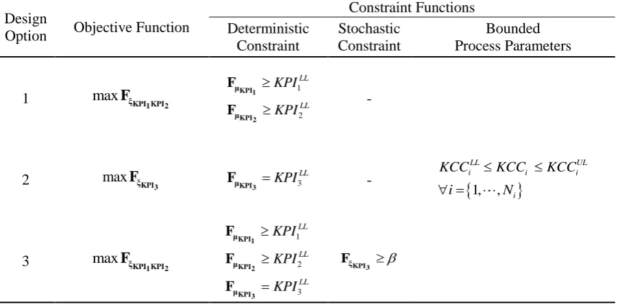
as multi–objective optimization. Table 8 describes the proposed optimization strategies for

various pre–defined KCCs/KPIs configurations.

Table 8 Proposed options for process parameters selection

Design

Option Objective Function

Constraint Functions Deterministic Constraint Stochastic Constraint Bounded Process Parameters

1 maxFξKPI KPI1 2

1 2 LL LL KPI KPI   KPI1 KPI2 μ μ F F -





LL UL

i i i

i

KCC KCC KCC

i N

 

 

2 maxFξ_KPI3 3

LL KPI  KPI3 μ F _-

3 maxFξKPI KPI1 2

18

6. Results and discussions 480

6.1 Statistical data analysis

The total number of KCCs, KPIs, experimental configurations, replication and dependent

KPIs are determined as Ni, Nj, Nk, Nl and d, respectively. The dependency among KPIs are 485

evaluated using the Pearson product-moment correlation coefficient test and its result () takes a value between +1 and −1, where 1 is total positive linear correlation, 0 is no linear correlation, and −1 is total negative linear correlation. The result of the Pearson test is given in Eq. (18).

According to results, dimple height (DH) and dimple upper surface area (DU) are chosen as

dependent KPIs and dimple lower surface area (DL) is independent from other KPIs. 490

  _{ }

cov ,

, 1, ,3

1 0.7852 0.2409

0.7852 1 0.5515

0.2409 0.5515 1

mn m n



 

  

 

 

  

 

 

m n

m n

KPI KPI

KPI KPI

(18)

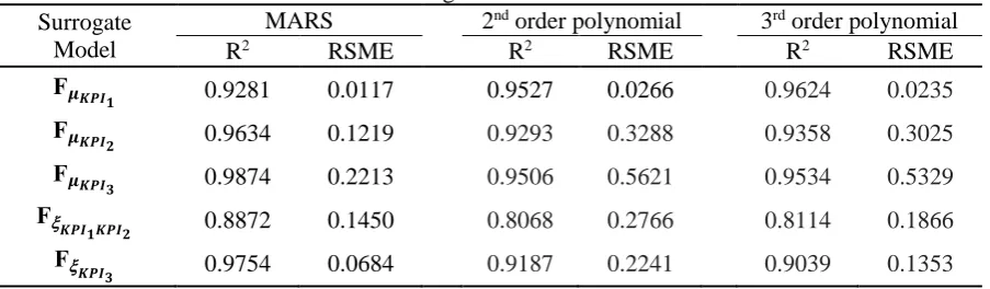
The goodness of surrogate models is assessed by computing the determination of coefficient

(R2) and root mean square error (RMSE) and the MARS models are compared with second and

495

third order polynomial regressions which are reported in

Table 9. The success rate in the stochastic case is not a binary value and it gets any value

between zero and one. However, its behaviour in one region inside the KCC–space cannot be

easily correlated to its behaviour in other region. This change can be handle by using piecewise

500

fitting methods and better R2 _{and RMSE are obtained in MARS model. The obtained MARS}

models and the measured KPIs are given in the in the Appendix.

Table 9 R2 _{& RSME values for different surrogate models}

Surrogate Model

MARS 2nd _{order polynomial 3}rd _{order polynomial}

R2 _{RSME R}2 _{RSME R}2 _RSME

F𝝁_{𝑲𝑷𝑰𝟏} 0.9281 0.0117 0.9527 0.0266 0.9624 0.0235

F𝝁_{𝑲𝑷𝑰𝟐} 0.9634 0.1219 0.9293 0.3288 0.9358 0.3025

F_𝝁

𝑲𝑷𝑰𝟑 0.9874 0.2213 0.9506 0.5621 0.9534 0.5329

F_

𝑲𝑷𝑰𝟏𝑲𝑷𝑰𝟐 0.8872 0.1450 0.8068 0.2766 0.8114 0.1866

F_

𝑲𝑷𝑰𝟑 0.9754 0.0684 0.9187 0.2241 0.9039 0.1353

19

6.2Deterministic Surrogate Models

510

In the deterministic scenario, the mean values are calculated to compute surrogate model

which estimates the KPI values over the KCC–space. The results of these deterministic

surrogate models are illustrated in Figs. 7 to 9 for varying scanning speed (SS) and incidence

angle () for constant laser track (LT) and focal offset (FO) values. These figures provide two

types of information; (i) the effect of the process parameters on KPIs which can be directly

515

used by the automotive industry; and, (ii) individual deterministic process capability spaces









interesting to note that dimple is formed in the same direction with laser track movement for

higher defocus (~5 mm) whereas dimple is formed in the opposite direction of the laser

movement for lower focal offset (~25mm). This behaviour is one of the findings of this study

520

and is shown in Fig. 10. It can be explained by the fact that larger defocusing generates bigger

laser beam spot size which leads to a drop in power intensity. In this case the molten material

is moved forward by the movement of the laser beam. The dimples obtained in this condition

are characterized by a cavity in the rear and higher dimple in front, which is highlighted in Fig.

2.

525

6.2.1 Characterization of dimple height (DH)

According to the literature, dimple height decreases with scanning speed. However, as

predicted in Fig. 7, this can only be obtained for high focal offset (~55 mm) and constant

530

incidence angle. For low focal offset (~25 mm), the laser track clearly affects the dimple height,

whilst a bipolarized pattern can be observed because of the mutual interaction between speed

and incidence angle. At medium focal offset (~35), scanning speed slightly affects dimple

height, whilst the interaction between laser track and incidence angle generates a unipolar

pattern. The highest dimple height is observed around 5 – 10 degrees. The reason for this could

535

be the amount of energy absorbed by the material and tilted keyhole that pushes the melting

upwards. It can be deduced that the dimple height increases while increasing laser track as also

20 540

Fig. 7.The estimated dimple height value (DH) over KCC–space in the deterministic scenario

6.2.2. Characterization of dimple upper surface area (DU)

Dimple upper surface area (DU) decreases with increasing scanning speed whist other

545

parameters are kept constant. However, it increases with increasing both scanning speed and

laser track but decreases with increasing both scanning speed and focal offset. It is evident that

increasing laser track results in higher and larger dimple since the longer displacement creates

longer trailing jet on the surface as also indicated in the literature [24]. The correlation patterns

exhibit a unipolar shape, which tends to be elongated moving toward higher laser track and

550

focal offset.

Fig. 8.The estimated dimple upper surface value (DU) over KCC–space in the deterministic scenario

555

6.2.3. Characterization of dimple lower surface area (DL)

It is interesting to note that the main and interaction effects of incidence angle into dimple

lower surface area (DL) can be negligible and it can be seen in Fig. 9 that the correlation pattern

21

correlated with focal offset and scanning speed. The minimum DL is observable for medium

(~35 mm) and high (~55 mm) focal offset and lower laser track (~ 2 mm).

Fig. 9.The estimated dimple lower surface value (DL) over KCC–space in the deterministic scenario

565

Fig. 10. Effect of focal offset on three KPIs when process parameters are constant at SS: 3 m/min, :

22

6.3 Deterministic Process Capability Space (DCP – Space)

The deterministic process capability space (DCp – Space) is illustrated in Fig. 11. The

575

shaded area represents the feasible region and any value inside corresponds to feasible process

parameters (KCCs) which simultaneously satisfy all quality requirements defined in Table 2.

According to the DCp – Space result, feasible process parameters cannot be achieved for lower

focal offset (~25 mm) since dimple lower surface area (DL) is more likely to exceed its

allowance limits that is highlighted in Fig. 9. The reason might be lower focal offset creates

580

higher power intensity and thus more amount of material is molten which results in wider and

deeper molten pool. The rate of change of the laser intensity determines the physical

phenomena between material and laser beam. For instance, slow speed, short laser track and

low focal offset result higher energy intensity rate and thus, higher dimple but larger dimple

lower surface area is occurred. Therefore, feasible regions are gathered in the medium level of

585

the process parameters.

Fig. 11. Deterministic Process Capability Space (DCP – Space) for laser dimpling process

590

6.4 Stochastic Process Capability Space (SCP – Space)

The calculated stochastic process capability space (SCp–Space) is presented in Fig. 12 It

represents the simultaneous product of the stochastic process capability spaces defined in Eq.

(16). The achievable success rates of the dimpling process are displayed in contour plot by

23

initially selecting minimal desirable success rate (β) at zero in Fig. 12. Therefore, it will provide

more information to select a set of KCCs. For example, point A and B are inside the feasible region in Fig. 11 which define two different sets of KCCs that simultaneously satisfy KPIs

allowance limits. On the contrary, these points represented in Fig. 12 are different success rates

since the process variation is less at the point B. Therefore, point B provide more robust process

600

parameters (KCCs) and SCp–Space can be utilized to select KCCs according to pre–defined

success rate (β). Furthermore, the deterministic process capability space and stochastic process

capability space have to follow same pattern since probability value is a function of mean and

variation.

According to results, higher success rate regions are concentrated at the medium focal offset

605

(~35 mm). The success rate is nearly zero at lower focal offset (~25 mm) thus confirming the

results obtained by the DCP–Space model. According to the results, the minimal desirable

success rate (β) was set at 0.8 and it was highlighted in shaded region in Fig. 12.

610

Fig. 12. Stochastic Process Capability Space (SCP – Space) for laser dimpling process

6.5 Process parameters selection and optimisation

Despite the fact that evolutionary algorithms do not guarantee the global optimum, their

615

convergence speeds to the optimal results (nearly global) are better than those of the traditional

techniques. Thus, evolutionary algorithms have been used for optimization of real-world

problems in many applications instead of traditional techniques [44–47]. Therefore, genetic

24

Population size, probability of crossover and mutation numbers were selected as 500, 0.60 and

620

0.12, respectively.

In this paper, we define three design options to optimize all KPIs which are described in

Table 8 and the optimization results are given in Table 10. The results indicate that the optimum

configurations are concentrated between medium (~35 mm) and high (~55 mm) focal offset

and higher laser track (~4 mm) and medium scanning speed (~3 mm). This can be explained

625

by the amount of time spent by the laser power intensity on the workpiece. It can be deduced

that by decreasing interaction time less amount of materials was molten and molten pool

becomes shallow because less amount of laser energy was absorbed. The design option three is approximately illustrated as Point C in Figs. 11 and 12.

630

Table 10 Optimization results

Design

Option SS  LT FO 𝜇̂𝐾𝑃𝐼1 𝜇̂𝐾𝑃𝐼2 𝜇̂𝐾𝑃𝐼3 ̂𝐾𝑃𝐼1⋯𝐾𝑃𝐼2 ̂𝐾𝑃𝐼3

1 2.0020 15.0069 3.9692 54.9941 0.198 2.756 4.868 1.000 0.000 2 3.3709 0.2704 3.0229 52.8982 0.092 0.710 0.000 0.283 1.000 3 3.9967 19.9778 3.4845 37.2153 0.199 1.592 0.000 1.000 0.993

In order to validate the optimization results obtained in Table 10 and estimated values from

the surrogate models defined in Eqs. (9), to (11), confirmation experiments were carried out by

coupon experiments. Five replications of each design option were performed on a 10 x 40 mm

635

sheet metal with a thickness of 0.75 mm and the results are reported in Table 11. It shows

measured 5 replications for each KPI and their mean and success rate. These values are

computed according to the methodological flow from Step 1 to Step 6.2 which are presented

in Table 7. These calculated values are compared against estimated values from the developed

surrogate models.

640

Table 11 Validation of the optimization results for all design options

Design

Option KPI Rep. 1 Rep. 2 Rep. 3 Rep. 4 Rep. 5 KPI ˆKPI KPI ˆKPI

1

DH 0.183 0.190 0.185 0.209 0.189 0.1912 0.198 1 1

DU 2.184 2.055 2.080 2.192 2.154 2.133 2.756 1 1

DL 4.467 4.318 4.415 5.028 3.417 4.329 4.868 0 0

2

DH 0.124 0.13 0.114 0.084 0.118 0.114 0.092 0.588 0.283 DU 1.123 1.186 1.037 0.776 1.076 1.0396 0.710 0.588 0.283

DL 0.000 0.000 0.000 0.000 0.000 0.000 0.000 1 1

3

25

These design options are offered to find robust process parameters to obtain maximum

dimple height and upper surface; and, minimum dimple lower surface area. The first option

studies maximizing mean and success rate of dimple height and upper surface area without

645

considering the dimple lower surface. According to the results, the calculated and estimated

mean and success rates are quite similar. However, this similarity is not achieved for the second

design option. The second option considers only to obtain robust parameters for minimum

dimple lower surface area. The variation of the DH and DU at this point are more than measured

values and dimple upper surface might be also correlated with dimple lower surface area. These

650

reasons might cause the different in the calculated and estimated values.

The laser dimpling process is currently utilized for the laser lap welding of zinc coated steels,

especially automotive industry. The dimples generate a small gap between faying surfaces

where the zinc vapour is vented out through. However, obtaining a constant gap without having

a darker spot at the back side of the steel are the major challenges of the process. An optimum

655

set of process parameter was validated by welding experiments and results are given in Fig. 13.

The figure shows images of welded specimen before and after the optimization of laser

dimpling process. The dark spots are not visible on the lower surface and there are no spatters

around the stitch after implementing optimum laser dimpling process parameters. Likewise,

the quality of weld seam is improved, no blow holes are detected in the weld seam.

660

Fig. 13 Remote laser welded joint. (a) – Trial and error approach before optimization. (b) –

Optimized configuration based on the proposed methodology 665

7 Conclusions and Final Remarks

This paper presents a novel methodology to select process parameters for laser dimpling

process. It is based on the process capability space which allows the estimation of a desired

process fallout rate in the case of quality failures or violation of process requirements. The

670