warwick.ac.uk/lib-publications
A Thesis Submitted for the Degree of PhD at the University of Warwick Permanent WRAP URL:
http://wrap.warwick.ac.uk/131745
Copyright and reuse:
This thesis is made available online and is protected by original copyright. Please scroll down to view the document itself.
Please refer to the repository record for this item for information to help you to cite it. Our policy information is available from the repository home page.
from a Genome-Wide Transcriptome and Methylome
Analysis of
Brassica oleracea
Jonathan Lewis Price
This thesis is submitted in partial fulfilment of the requirements for the degree of
Doctor of Philosophy
University of Warwick, Department of Life Sciences
I would like to extend my gratitude to my supervisor, Dr. Jose Gutierrez-Marcos, for
giving me this opportunity and allowing me to develop my knowledge and skills under
his guidance on so many projects. You really have been a source of inspiration and
great ideas.
I would also like to thank my advisory panel, Dr. Sascha Ott and Dr. Graham
Teakle for their generous time and advice. My thanks also goes to everyone in the
Marcos group over the last 4 years many of whom have kept me sane with sound
advice in work and evenings at the local. Without you the four years would have been
even harder.
I also need to thank my parents, Dean and Linda Price, for their support over
the last 28 years. Particularly the encouragement to go to University, without that,
this would not have been possible. I would also like to thank my partner in crime,
Grace Watkins who has been a source of calm and understanding throughout, it really
wouldn’t be the same without you. Also for those late nights of correcting my
atro-cious spelling, so on that note I would also like to thank Ruth Watkins for her literary
skill and punctuation policing.
Lastly, I would like to thank the BBSRC and the MIBTP program, I have really
developed throughout the 4 years of my PhD and it would not have been possible
The work herein has not been published in a peer reviewed journal. However
during my PhD I was able to contribute significantly to a number of projects. Although
not assessed for this degree, the funding received from the BBSRC has allowed this
research to be conducted.
• Price, J., Harrison, M., Hammond, R., Adams, S., Gutierrez-marcos, J.,
Mal-lon, E. (2018). Alternative splicing associated with phenotypic plasticity in the
bumble bee Bombus terrestris. Molecular Ecology.
• Wibowo, A., Becker, C., Durr, J., Price, J., Papareddy, R., Santain, Q., Spaepen,
S., Hilton, S., Bending,G., Schulze-Lefert, P., Weigel., D, and
Gutierrez-Marcos, J. (2018). Incomplete reprogramming of cell-specific epigenetic marks
during asexual reproduction leads to heritable phenotypic variation in plants.
PNAS.
• Wibowo, A., Becker, C., Marconi, G., Durr, J., Price, J., Hagmann, J., Papreddy,
R., Putra, H., Kageyama, J, Becke,r J., Weigel, D., Gutierrez-marcos, J. (2016).
Hyperosmotic stress memory in Arabidopsis is mediated by distinct
epigeneti-cally labile sites in the genome and is restricted in the male germline by DNA
This thesis was submitted to the University of Warwick for the degree of Doctor of
Philosophy. The work presented here is original and has not been considered for any
other award. All work here in was performed by myself with few exceptions outlined
below.
Mr. Robert Maple, Dr. Yang Seok, Mr. Ranjith Papareddy (University of
Warwick)
Assisted in the growth and harvesting of samples along with the extraction of RNA
and DNA for sequencing.
Max Plank Institute, T ¨ubingen
The sequencing facility at MPI T¨ubingen performed the library preparation and
the sequencing of the libraries.
Warwick Crop Centre
Also assisted in the growth of the samples, management of the greenhouses and
from a Genome-Wide Transcriptome and Methylome
Analysis of
Brassica oleracea
Abstract
With global food insecurity on the rise and increased pressures on habitat
conser-vation it is vital to pursue increased efficiencies in plant breeding. New understanding
of genetics in the last five decades has provided significant advances in yield gains
in most cultivated crops. However, new advances in genomics have opened the door
to better design breeding programs; the major strategy to develop new cultivars, in
order to exploit novel sources of genetic variation and increase selection efficiency.
Many studies have focused on the efficient use of molecular markers to speed up
se-lection processes, yet the use of omics studies in plant breeding programs is currently
under utilised as they could be used to elucidate the mechanisms underpinning the
inheritance of traits currently exploited by plant breeders. This study has generated
whole-genome transcriptome and methylome data to uncover the mechanisms
impli-cated in the inheritance of traits generated during a doubled haploid (DH) breeding
program. Our analysis reveals the existence of a number of predictive elements that
explain the molecular variation present in DH breeding. The major elements
con-tributing to this variation are the level of dominance in hybrids and the contribution
of each parental genome in individual DH lines. Collectively, our works demonstrate
that genomic and epigenomic studies can provide insights into genome regulation and
• DNADeoxyribonucleic Acid
• RNARibonucleic Acid
• mRNAMessenger ribonucleic Acid
• siRNASmall ribonucleic Acid
• siRNASilencing ribonucleic Acid
• miRNAMicro ribonucleic Acid
• ncRNANon-coding ribonucleic Acid
• MABMarker assisted breeding
• MASMarker assisted selection
• NGSNext generation sequencing
• RNASeqRibonucleic Acid sequencing
• BSSeqBisulphite Sequencing
• QTLQuantitative trait loci
• RFLPRestriction fragment length polymorphism
• SSRSmall sequence repeat
• SNPSingle nucleotide polymorphism
• GCAGeneral combining ability
• SCASpecific combining ability
• GSGenomic selection
• MPVMid parent value
• HPHigh parent
• LPLow parent
• TFTranscription factor
• TETransposable element
• 5meC5 methyl cytosine
• GSGenomic selection
• gbMGene body methylation
• FDRFalse discovery rate
• DEGDifferentially expressed gene
• phDEGParent hybrid differentially expressed gene
• dhDEGDoubled haploid differentially expressed gene
• DMRDifferentially methylated region
• MRMethylated region
• ELDExpression level dominance
• MLDMethylation level dominance
1 Introduction 1
1.1 Plant Breeding . . . 1
1.1.1 From Breeding to Molecular Breeding . . . 1
1.1.2 Hybridisation . . . 5
1.1.3 Doubled Haploids . . . 7
1.1.4 Typical Modern Breeding Strategies . . . 9
1.2 Genome Regulation in Plants . . . 13
1.2.1 Gene Expression . . . 13
1.2.2 DNA Methylation . . . 15
1.3 Merging Plant Genomes . . . 19
1.4 Genomic Analyses inBrassicaSpecies . . . 21
1.5 Aims and Hypothesis . . . 23
2 Methods 25 2.1 Creation of F1 and Doubled Haploid Lines . . . 25
2.2 Selection of Samples and Plant Growth . . . 26
2.3 RNA Extraction Data Generation . . . 27
2.4 RNASeq Data Processing . . . 28
2.6 Bisulphite Data Processing . . . 29
2.7 Single Cytosine Analysis . . . 30
2.8 Methylated Regions . . . 30
2.9 Differentially Methylated Regions . . . 31
2.10 Parent and Hybrid Differential Expression and Methylation . . . 32
2.11 Homologous Recombination Site Detection . . . 35
2.12 Differential Expression and Methylation in the DHLs . . . 38
2.13 Gene Ontology Analysis . . . 38
2.14 Intersection of DMRs and Genes and Transposons . . . 38
3 Transcriptome and Methylome Analysis of A12Dhd and GDDH33 Parental Lines 42 3.1 Introduction . . . 42
3.2 Chapter Aims and Hypothesis . . . 46
3.3 Mapping of Parental Accessions to the ReferenceB. oleraceaGenome 47 3.4 Gene Expression Differences Between A12Dhd and GDDH33 . . . . 47
3.5 Methylation Analysis in the Parental Lines . . . 51
3.5.1 Analysis of Single Cytosines . . . 51
3.5.2 Differentially Methylated Regions between A12Dhd and GDDH33 . . . 53
3.6 Discussion . . . 55
4 Transcriptome and Methylome Analysis of the F1 Hybrids 57 4.1 Introduction . . . 57
4.1.2 Epigenetic Studies of F1 Hybrid . . . 61
4.2 Chapter Aims and Hypothesis . . . 65
4.3 Gene Expression in the Parent Hybrid Cross . . . 66
4.3.1 Gene Expression Dynamics in the F1 Hybrid . . . 66
4.3.2 Differentially Expressed Genes . . . 69
4.4 Methylation in the Parent Hybrid Cross . . . 72
4.4.1 Analysis of Single Cytosines . . . 72
4.4.2 DMR Dynamics in the F1 Hybrid . . . 76
4.4.3 Location of Methylation and Differential Methylation . . . 80
4.5 Discussion . . . 83
5 Transcriptome and Methylome Analysis of the Doubled Haploid Lines 87 5.1 Introduction . . . 87
5.2 Chapter Aims and Hypothesis . . . 90
5.3 Genotyping Doubled Haploid Lines - Understanding the Parental Genome Contribution . . . 92
5.4 Gene Expression Dynamics in the DH lines . . . 101
5.5 Differentially Expressed Genes in the DH Lines . . . 105
5.6 Methylation Dynamics in the DH Lines . . . 107
5.7 Correlation Between DNA Methylation and Gene Expression in B. oleraceaDH Lines . . . 114
5.8 Discussion . . . 120
6.1 Parental Regulome Divergence Governs Parental Combining Ability
for mRNA Dosage Dependant Traits . . . 127
6.2 Exploiting the Expression-level Dominance in Plant Breeding
Pro-grams for mRNA Dosage Dependant Traits . . . 129
6.3 Utilising Parental Genome Contribution in Homozygous Line
Selec-tion . . . 131
6.4 Future Directions . . . 132
6.4.1 Parental Genome Contributions in Doubled haploid breeding . 132
6.4.2 Studies of Genome Mergers . . . 135
Appendices 160
A Read Processing Numbers 161
1.1 Simplified schematic of typical breeding strategies. Arrows
indi-cate the movement of potential cultivars through the breeding program. 12
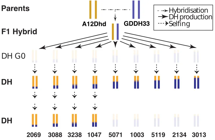
2.1 Schematic of samples in this study along with their method of
creation. Samples in bold indicate those with whole genome
bisul-phite sequencing data and whole genome RNA sequencing data. Line
names or numbers are shown underneath each line and the arrows
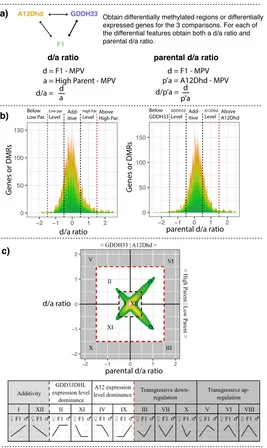
2.2 Schematic showing how the d/a and parental d/a ratios are
calcu-lated and plotted. The ratios are used to show how the dynamics
of a DMR or gene in F1 hybrid relate to the parental methylation
or expression. a) The calculation of the ratios. Firstly, three
pair-wise comparisons are performed (A12Dhd - F1, GDDH33 - F1 and
A12Dhd - GDDH33). Then for each of these genes or DMRs shown
to be significant in at least one comparison, two ratios are calculated.
The d/a ratio and the parental d/a ratio. b) Displays the meaning of the
ratios. The d/a ratio (left histogram) describes the methylation of the
DMR or expression of the gene in the F1 according to the high or low
parent (parent with highest or lowest expression). The parental d/a
ra-tio (right histogram) describes the methylara-tion of the DMR or
expres-sion of the gene in the F1 according to the expresexpres-sion of the maternal
parent (A12Dhd) or the paternal parent (GDDH33). The histograms
show the thresholds imposed on these ratios that decide the expression
or methylation category (additive, parental-level dominance or above
/ below parental levels. c) Plotting and display of the ratios and
cate-gories. In the top plot, each genes ratios are plotted, the d/a ratio on
the y-axis and the parental d/a ratio is plotted on the x-axis. Plotting
in this way, each differentially expressed feature can be categorised
according to both the high / low parent and the maternal / paternal
par-ent. The bottom table of c) shows this categorisation. Roman
numer-als show the categories as they are commonly described (Yoo et al.,
2013). Underneath the Roman numerals in the table, there is a graphic
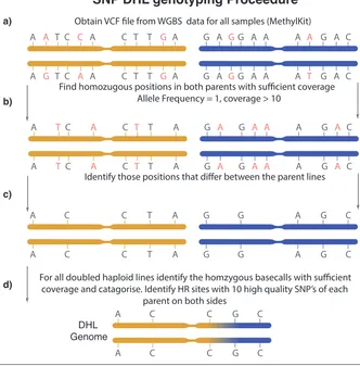
2.3 Schematic of SNP genotyping pipeline. a) From vcf files of each
parental genome (A12DHd - yellow, GDDH33 - blue), positions in
each genome are only kept if their allele frequency is equal to 1 and
their coverage is greater than 10. b) Positions between the parental
genome are compared, they are kept if the base call in each parental
genome is different and both genomes have received greater than 10
coverage. c) This is the set of distinguishing positions that can separate
the DH genomes. d) The final step of the program introduces the vcf
file from a DH line and looks for positions with an allele frequency
of 1, it then categorises each position according to the set of parental
SNPs identified earlier. The program identifies a HR site if there is a
switch in the parental inheritance with 10 SNPs on either side of the
HR site. . . 37
2.4 Three examples of possible intersections from the GFF intersector
program. a) The case in which there is a gene which is overlapped
by 5 DMRs, this becomes an intersect regions containing 1 gene and
5 DMRs. b) The intersect regions contains 2 genes and 4 DMRs, the
two genes are contained within one region because they are less than
the user supplied flanking region (f) apart and both gene has at least 1
DMR intersecting. c) In this example the second gene is not included
in the intersect region because it has no associated DMRs within f of
the TSS or TES. Yellow boxes show user defined regions e.g DMRs.
Blue boxes show exons of genes, the TES and TSS are defined in the
2.5 Schematic showing the process of correlating gene expression and
DMR methylation within regions identified using the
GFFInter-sector program. a) Shows the first step of correlation program in
which DMRs of the same sequence context that directly overlap are
combined into DMR blocks. b) Correlation of the DMR blocks and
genes. Correlations are made between all DMR blocks and any gene
within the flanking region of the DMR block, this maybe more than
one gene. For each gene and DMR block comparison (5 in the above
example), the coverage in methylation in each sample is assessed to
ensure 5 reads are covering the region in at least 5 samples. Then
the gene is checked for expression in at least one sample and a 1.2
fold difference. Then for each comparison identified, Spearman’s rank
correlation is performed. From all comparisons those with are FDR of
less than 0.01 are considered significant. . . 41
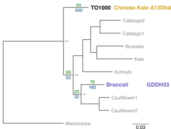
3.1 Genetic distance betweenB oleraceavarieties. Dendrogram,
modi-fied from Golicz et al. (2016) shows the genetic distance between the
9 lines used by Golicz et al. (2016). Numbers in green show genes that
are present in the varieties below that node but not present in the
oth-ers. The blue numbers represent the number genes that are not present
in the lines below that node but present in the other lines. The scale
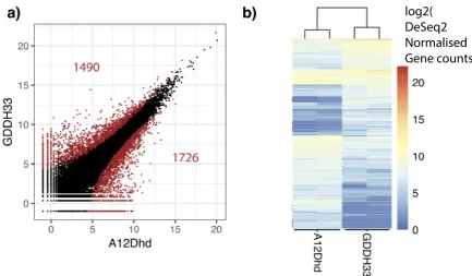
3.2 Parental differentially expressed genes. a) Scatter plot showing the
average of each replicates expression of each gene for A12Dhd and
GDDH33 with significant pDEGs appearing in red. b) Heatmap
dis-playing expression of the 3216 parental DEGs with hierarchical
clus-tering. . . 48
3.3 Global cytosine methylation in A12Dhd and GDDH33 in each
methylation context. CG (top), CHG (middle) and CHH (bottom).
a) Histogram displaying the proportion of sites exhibiting
methyla-tion ratios of 0-100% the panel in the corner of each plot displays a
zoomed view of the distribution of sites with 1-100% methylation. b)
The average methylation percentage of all cytosines. . . 52
3.4 Average methylation across genomic features for CG, CHG and
CHH methylation. Genes (Left), DNA and RNA transposable
ele-ments (Right). For each feature and context the 2 kb flanking regions
for each feature are an average methylation value for a particular
po-sition for each feature in the genome. Across the feature body each
feature is split into 100 bins and the methylation is averaged over these
3.5 Numbers and location of pDMRs and pMRs.a) Barplot of the
num-bers of DMRs between A12Dhd and GDDH33 in each sequence
con-text. DMRs with higher methylation in A12Dhd are shown in yellow
and DMRs with higher methylation in GDDH33 are shown in blue.
b) Location of these DMRs within genomic features, each base of a
set of DMRs is assigned to the feature that it overlaps with. Then
the results are displayed as a percentage of the total bases in that set.
For each sequence context both A12Dhd MRs and GDDH33 MRs are
shown. Then the DMRs between these two genotypes are split into
DMRs with higher methylation in A12Dhd (A12) and DMRs with
higher methylation in GDDH33 (GD). WG refers to the assignment
of all the bases in the reference genome when assigned to a feature.
This is done in a hierarchical fashion to account for overlapping
fea-tures (gene, transposon, upstream, downstream, intergenic: in order of
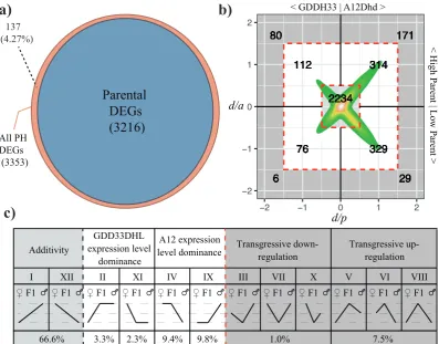
4.1 Gene expression dynamics in F1 hybrid. a) Venn diagram
show-ing parental DEGs (blue) from the comparison between A12Dhd and
GDDH33. Then the parental and hybrid DEGs (brown) from all 3
comparisons (A12Dhd - F1, GDDH33 - F1 and A12Dhd - GDDH33).
This plot shows there is little novel differential expression in the F1
hybrid. b) Dominant-to-additive plot showing expression dynamic
of phDEGs in F1 hybrid relative to the parental expression. Each
phDEGs ratios are plotted, the d/a ratio on the y-axis and the parental
d/a ratio is plotted on the x-axis. Plotting in this way, each phDEG
can be categorised according to both the high / low parent and the
ma-ternal / pama-ternal parent as shown by the numbers in the quadrants of
the graph. c) Shows the categorisation of each gene. Roman
numer-als show the categories as they are commonly described (Yoo et al.,
2013). Underneath the Roman numerals in the table, there is a graphic
displaying the expression or methylation pattern of this category for
the 3 genotypes (A12Dhd - maternal, GDDH33 - paternal and F1)
then underneath that are the proportions of the phDEGs belonging to
12 mutually exclusive expression patterns. . . 67
4.2 Heatmaps of phDEGs. The F1 genotype forms a clade with
A12Dhd for additively and non-additively expressed genes. a)
Heatmap of additive phDEGs. b) Heatmap of non-additively
ex-pressed phDEGs. Scale displayed is log2(DESeq2 normalised
expres-sion levels). Hierarchical clustering was performed and displayed as a
4.3 Global cytosine methylation in A12Dhd, GDDH33 and F1 in each
methylation context. CG (top), CHG (middle) and CHH (bottom).
a) Histogram displaying the proportion of sites exhibiting methylation
ratios of 0-100% the panel in the corner of each plot displays a zoomed
view of the distribution of sites with 1-100% methylation. b) The
average methylation percentage of all cytosines. . . 74
4.4 Methylation average across genomic features for CG, CHG and
CHH methylation. Genes (Left), DNA and RNA transposable
ele-ments (Right). For each feature and context the 2 kb flanking regions
for each feature are an average methylation value for a particular
po-sition for each feature in the genome. Across the feature body each
feature is split into 100 bins and the methylation is averaged over these
bins and then averaged across all features for these bins . . . 75
4.5 Venn diagrams showing overlap between pDMRs (blue) and
phDMRs (brown). The F1 has little novel methylation at CG sites
but more novel methylation at CHG and CHH sites.For each
con-text separately the pDMRs are obtained from the comparison between
A12Dhd and GDDH33 and the phDMRs are obtained from the three
4.6 Methylation dynamics for CG, CHG and CHH context phDMRs.
a) Dominant-to-additive plots showing methylation dynamics of
phDMRs in F1 hybrid relative to the parental methylation. Each
phDMRs ratios are plotted, the d/a ratio on the y-axis and the parental
d/a ratio is plotted on the x-axis. Plotting in this way, each phDMR
can be categorised according to both the high / low parent and the
maternal / paternal parent as shown by the numbers in the quadrants
of the graph. b) Shows the categorisation of each phDMR. Roman
numerals show the categories as they are commonly described (Yoo
et al., 2013). Underneath the Roman numerals in the table, there is a
graphic displaying the expression or methylation pattern of this
cate-gory for the 3 genotypes (A12Dhd - maternal, GDDH33 - paternal and
F1) then underneath that are the proportions of the phDMRs belonging
to 12 mutually exclusive expression patterns in each sequence context. 78
4.7 Heatmaps of phDMRs. Methylation of the F1 is most similar to
A12Dhd for both additive and non-additive phDMRs. a) Additive
phDMRs. b) Non-additive phDMRs. For each sequence context; CG,
4.8 Location of phMRs and phDMRs at CG, CHG and CHH context
within genomic features. A - Additive phDMRs, N - Non-additive
phDMRs, T - Trangressive phDMRs. Mr - MRs from relevant context.
WG - The reference genome if all bases were assigned to a feature. All
bases of a particular feature set are assigned to a genomic feature and
then plotted as a percentage of the total number of bases in that feature
set. This is done in a hierarchical fashion to account for overlapping
features (gene, transposon, upstream, downstream, intergenic: in order
of decreasing importance). . . 81
4.9 Locations of phDMRs and phMRs in different transposon types.
In each case it shows the proportion of bases in each feature type that
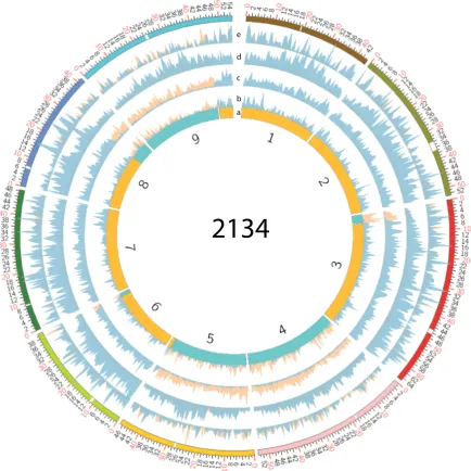
5.1 Large example of circos plots for whole genome comparisons.
Whole genome comparisons between any DH line and either
par-ent are invalid, illustrates the need to only compare inherited
re-gions between the parents and DH lines. Results from all DH lines
tested can be seen in Figures 5.2, 5.3, although smaller they are
just there to illustrate the point mentioned above. Whole genome
comparison of the DH line 2134 and GDDH33 in blue. Then whole
genome comparison of DH line 2134 and A12Dhd in yellow. a)
Pre-dicted genotype of the DH line. b) Magnitude of DEGs between the
DH line and both parents. c) Magnitude of CG DMRs between the
DH line and both parents. d) Magnitude of CHG DMRs between the
DH line and both parents. e) Magnitude of CHH DMRs between the
DH line and both parents. The outer ideogram displays the
chromo-some coordinates in megabases along with the centromere positions
5.2 Circos plots for whole genome comparisons. Whole genome
com-parisons between any DH line and either parent are invalid,
il-lustrates the need to only compare inherited regions between the
parents and DH lines. DH line vs GDDH33 in blue and DH line
vs A12Dhd in yellow. a) Predicted genotype of DH lines. b)
Magni-tude of DEGs between the DH lines and both parents. c) MagniMagni-tude
of CG DMRs between the DH lines and both parents. d) Magnitude
of CHG DMRs between the DH lines and both parents. e)
Magni-tude of CHH DMRs between the DH lines and both parents.The outer
ideogram displays the chromosome coordinates in megabases along
with the centromere positions as a white band. . . 94
5.3 Circos plots for whole genome comparisons. Whole genome
com-parisons between any DH line and either parent are invalid,
il-lustrates the need to only compare inherited regions between the
parents and DH lines. DH line vs GDDH33 in blue and DH line vs
A12Dhd in yellow. a) Predicted genotype of DH lines. b) Magnitude
of DEGs between the DH lines and both parents. c) Magnitude of
CG DMRs between the DH lines and both parents. d) Magnitude of
CHG DMRs between the DH lines and both parents. e) Magnitude
of CHH DMRs between the DH lines and both parents. The outer
ideogram displays the chromosome coordinates in megabases along
5.4 Plots of results from SNP genotyping and epigenotyping. For each
chromosome the observed parent of origin is shown as 4 bars
(yel-low - A12Dhd, blue - GDDH33). Bars from top to bottom - SNP
data genotype, 60kb epigenotyping, 70kb epigenotyping and 150kb
epigenotyping. . . 98
5.5 Plots of results from SNP genotyping and epigenotyping. For each
chromosome the observed parent of origin is shown as 4 bars
(yel-low - A12Dhd, blue - GDDH33). Bars from top to bottom - SNP
data genotype, 60kb epigenotyping, 70kb epigenotyping and 150kb
epigenotyping. . . 99
5.6 Plots of results from SNP genotyping and epigenotyping. For each
chromosome the observed parent of origin is shown as 4 bars (yellow
-A12Dhd, blue - GDDH33). Bars from top to bottom -SNP data
geno-type, 60kb epigenotyping, 70kb epigenotyping and 150kb
epigenotyp-ing. . . 100
5.7 Genotypes of DH lines. a) Percentage of parental genome inheritance
to each DH line. b) Circos plot. Each ring represents the diploid
genome of a DH line. Each chromosome is coloured according to it’s
5.8 Dynamics of dhDEGs in each of the parentally inherited genomes
from each DH line.a) There are more dhDEGs on GDDH33 inherited
genomes compared to A12Dhd inherited genomes (T-test (t = -2.047,
p-value = 0.03174)). b) Venn diagram with the parental and hybrid
DEGs identified in Chapter 4 and the DH DEGs from each line, split
by parental inheritance and their overlapping genes. c) Shows the F1
expression dynamics of the phDEGS that overlap with dhDEGs (A =
phDEGs and A12Dhd inherited dhDEGs, G = phDEGs and GDDH33
inherited dhDEGs) and the phDEGs that recover in the DH lines (R)
these are sections shown in the venn diagrams in panel b. There is a
significant association between F1 expression and dynamics and the
catagory of DEG - X2(df = 4, N = 3254) = 145.7, p-value<0.001. . . 102
5.9 Parental dominant-to-additive ratios of the dhDEGs, for each
in-herited genome dhDEGs tend to display expression dynamics
sim-ilar to that of the other parental genome . From left to right; Top
-2069, 3088, 3238, Middle - 1047, 5071, 1003, Bottom - 5119, 2134,
3013. For each line their A12Dhd inherited dhDEGs are shown in
yellow and the GDDH33 inhertied dhDEGs are shown in blue. The
x-axis displays the parental d/a ratio, a ratio of 1 would mean a gene
has equal expression to the gene in A12Dhd and a ratio of -1 means
5.10 There is a negative relationship between relative gene expression
change and whole genome inheritance in the DH lines. For each
inherited genome in each DH line the relative gene expression change
(dhDEGs per gene inherited) is plotted against the amount of genome
inherited from that parent. The significant relationships are shown as
lines calcuated by linear regression. . . 104
5.11 Combined GO analysis for dhDEGs, each node represents an
en-riched GO term.(FDR<0.05). Size of node and label represents the
number of DH lines a given terms is enriched in. . . 106
5.12 Comparison of CG, CHG and CHH dhDMRs with the phDMRs.
a) Venn diagram with the parental and hybrid DMRs identified in
Chapter 4 and the dhDMRs from each line, split by parental
inheri-tance and their overlapping DMRs. b) Shows the F1 expression
dy-namics of the phDMRs that overlap with dhDMRs (A = phDMRs and
A12Dhd inherited dhDMRs, G = phDMRs and GDDH33 inherited
dhDMRs) and the phDMRs that recover in the DH lines (R) these are
sections shown in the venn diagrams in panel a. There is a
signifi-cant association between F1 methylation dynamics and the category
of DMR -(CG = X2 (df = 4, N = 22807) = 465.5, p-value <0.001),
(CHG = X2(df = 4, N = 11946) = 483.6, p-value<0.001), (CHH = X2
5.13 Number of dhDMRs in each line split by parental inheritance for
each sequence context.There are more CG dhDMRs on A12Dhd
in-herited genome sections than GDDH33 genome sections (CG - T-test
(t = -2.224, p-value = 0.0485)). CHG and CHH inherited sections do
not show significant differences (CHG - (t = 0.601, p-value = 0.5583),
CHH - (t = 0.743, p-value = 0.4689)) . . . 110
5.14 Relationship between parental genome dosage and epigenetic
changes in DH lines. For each inherited genome in each DH line
the relative gene methylation change (dhDMRs per MR inherited) is
plotted against the amount of genome inherited from that parent. The
significant relationships are shown as lines calcuated by linear
regres-sion. Non significant relationships are shown as a faint line. . . 111
5.15 Locations of dhDMRs in different genomic features. Each base of
the DMRs are assigned to the genomic feature that it overlaps with in
the annotation, these are displayed as a proportion of the total bases of
that DMR category. This is done in a hierarchical fashion to account
for overlapping features (gene, transposon, upstream, downstream,
in-tergenic: in order of decreasing importance) . . . 112
5.16 Locations of dhDMRs in different transposon types. Each base of
the DMRs is assigned to the transposon type that it overlaps with in
the annotation, these are displayed as a proportion of the total bases of
5.17 The methylation contexts of the dhDMRs differ in their
distribu-tion across genes with which they overlap. Density plot showing
the distribution of dhDMRs in each sequence context over genes. For
each feature and context the 2 kb flanking regions show the number
of DMRs that are assigned to a particular position for each feature in
the genome. Across the gene body each gene is split into 100 bins and
the plot displays the number of DMRs that reside in that bin from all
features. . . 115
5.18 Methylation and expression of the Agamous-like locus. The left
hand side shows single base resolution methylome of the available
samples for this region. The right hand side shows the expression of
this locus in the available samples. Bars are coloured to show the
genotype of this locus. . . 116
5.19 Aligned reads for Agamous-like locus does not follow the Parkin
et al. (2014) annotation.This plot shows aligned reads from all
sam-ples for this locus. It shows that there is little evidence for the exon
boundaries found in the official annotation. However there are
tran-scripts produced from this locus. The annotation for Agamous-like is
shown in blue at the bottom. The coordinates for chromsome 6 are
shown above and then the aligned reads for all samples are shown in
red with the number of reads from these that actually support the
5.20 Methylation and expression of the FAS4 locus. The left hand side
shows single base resolution methylome of the available samples for
this region. The right hand side shows the expression of this locus in
the available samples. Bars are coloured to show the genotype of this
locus. . . 118
5.21 Methylation and expression of the TIL locus. The left hand side
shows single base resolution methylome of the available samples for
this region. The right hand side shows the expression of this locus in
the available samples. Bars are coloured to show the genotype of this
locus. . . 119
6.1 Simplified schematic of typical breeding strategies. Arrows
indi-cate the movement of potential cultivars through the breeding
3.1 Phenotipic measurements of A12DHd and GDDH33 made by
Ng-wako (2003), raw data was unavailable and so actual measurements
are approximated here. Parent in bold shows the parent with
high-est value of that trait at that time point. The measurements are given
below are the average measurement. (GDDH33 - A12Dhd) . . . 44
3.2 GO analysis of 1726 genes with higher expression in A12Dhd
com-pared to GDDH33.All terms achived FDR<0.05. . . 49
3.3 GO analysis of 1490 genes with higher expression in GDDH33
compared to A12Dhd.All terms achived FDR<0.05. . . 50
4.1 GO analysis of 2234 additively expressed F1 genes. All terms
achived FDR<0.05 . . . 70
4.2 GO analysis of 1119 non additively expressed F1 genes. All terms
achived FDR<0.05 . . . 71
A.1 Table displaying the raw read numbers and the number after
processing of the reads and alignment to the reference genomes.
A.2 Table displaying the raw read numbers and the number after
processing of the reads and alignment to the reference genomes.
RNASeq libraries - New batch. . . 163
A.3 Table displaying the raw read numbers and the number after
pro-cessing of the reads and alignment to the reference genomes.
BS-Seq libraries - Original old batch. . . 164
A.4 Table displaying the raw read numbers and the number after
pro-cessing of the reads and alignment to the reference genomes.
BS-Seq libraries - New batch. . . 165
B.1 Regression statistics. Relative gene expression change and genome
ownership. . . 167
B.2 Regression statistics.Relative CG and CHG methylation change and
genome ownership. . . 168
B.3 Regression statistics.Relative CHH methylation change and genome
Introduction
1.1
Plant Breeding
1.1.1 From Breeding to Molecular Breeding
The earliest evidence of human driven selection on plants dates from around 12,000
years ago. In G¨obekli Tepe, Turkey it is believed that Triticum monococcumwas
se-lected over the natural einkorn wheat because its tough spindle allowed easy harvest
and threshing. This has now been shown to have a monogenic basis, so these
prehis-toric humans selected this gene which, without human requisite, would be
disadvan-tageous (Schlegel, 2018). This selection of beneficial traits by humans has occurred
in every civilisation and has resulted in the wide array of edible plants available today.
The scientific documentation of agriculture and horticulture was taken up in the
an-cient cultures and even before 1 AD there was knowledge of grafting, clonal
propaga-tion and selecpropaga-tion. However, plant breeding in a systematic way was only undertaken
after the discovery of gender in plants by Rudolf Camerarius in 1694, which allowed
Dianthus caryophyllus andDianthus barbatus was reported by Thomas Fairchild in
1717. However, in these early times, the concepts of genes and chromosomes were not
available and so it was an empirical science based on fine observations and ”breeders
experience” without a theoretical background. The theory was not applied to these
methods until 1900, when the ’Experiments on Plant Hybridization’ was confirmed,
having originally been written in 1865 by Gregor Mendel. This meant an explosion of
new varieties and the birth of quantitative genetics.
The next large advance in breeding came in the ’green revolution’ in the
mid-twentieth century. At this time, advances in health care meant that the population was
increasing. In Asian countries, much of the suitable agricultural land was already in
use (Khush, 2001). This necessity led to the development of new technologies for
plant breeding, particularly in rice, maize and wheat. The gains came from
system-atically targeting many different characteristics including; yield stability, stress
resis-tance (biotic and abiotic), environmental adaption and quality. This was combined
with an increase in knowledge of mechanical farming, genetics, chemical applications
and more stable irrigation. This, and a forceful social reform strategy and propaganda
campaign led by the West resulted in increased yields world-wide. The food and
agri-cultural agency reported that in the two decades between 1965 and 1985, crop yields
per hectare improved by 56 percent. The techniques of artificial crossing,
hybridisa-tion, induced mutation and tissue culture were all used during this time and created
many cultivars, such as IR8; developed in 1967 by the Indian rice breeder Nekkanti
Subba. It offered yields of 10 tons per hectare where it was common to expect only
1.5 tons per hectare (Schlegel, 2018). But after the gold rush of gains, yield growth
phe-notypic observation. Quantitative traits on the other hand, are controlled by multiple
loci and do not segregate in a mendelian fashion often resulting in continuous
pheno-types. This makes isolating the underlying genetic factors very difficult (Walley et al.,
2012).
Now arguably we are in the next agricultural era: the era of post-genomic science.
The discovery of restriction fragment length polymorphism (RFLP) in the 1980s
al-lowed the use of molecular markers to improve selection efficiency in plant breeding
programs (Botstein et al., 1980). Later the use of PCR meant that simple sequence
repeat (SSR) markers took over (Mullis et al., 1986). These genomic markers were
highly automatable and cheaper per data point. For example; Monsanto switched to
a fully automated single nucleotide polymorphism (SNP) based genotyping system.
Then from 2000 to 2006 data production increased 40-fold whilst the cost per data
point decreased 6-fold (Eathington et al., 2007).
With next generation sequencing becoming common place, more ways of
exploit-ing the genetic code are becomexploit-ing apparent and now, marker assisted breedexploit-ing (MAB)
forms the basis for many modern breeding programs. The techniques are required
be-cause many important polygenic traits cannot be harnessed with mendelian methods.
This is because quantitative traits are controlled by multiple loci, known as
quanti-tative trait loci (QTLs). The first stage of MAB programs rely on identifying DNA
markers closely linked to the phenotypes of interest. These techniques rely on the fact
that the distance between two loci causing a segregating phenotype is proportional to
the pattern of segregation of the alleles in later generations. After a genetic map has
identify the markers needed for selection. QTL analysis exploits these principles by
genotyping; segregating populations nearly inbred lines, recombinant inbred lines and
doubled haploid lines to identify markers that co-segregate with the phenotype. New
methods like expressionQTL, epiQTL and proteinQTL are also ways of selecting the
cause of a trait (Moose and Mumm, 2008). Along with identifying the underlying
genetic cause of traits, DNA genotyping from young plants is much less work than
phenotyping older plants (Butruille et al., 2015). However, these methods also suffer
from many false positives and the population size required is large. In bigger crop
species with long life cycles, growth space and maintenance is a big cost, along with
the labour required for the phenotyping studies. Being able to genotype quickly
in-creases the number of breeding cycles possible per year, meaning that even with the
advanced technology required it is still more cost effective.
The next generation sequencing (NGS) platforms allow single base resolution of
any genome. Now many genomes are sequenced providing the groundwork for omics
studies across many taxa. Better resolution of techniques means that we are able to
have a deeper understanding of the mechanisms underpinning the phenotypic
obser-vations seen in plant breeding. Omics studies can be focussed at the DNA, but also
at the gene level with transcriptional studies and at the epigenetic level. Using these
methods alongside traditional ones gives greater understanding of the actual causes of
the phenotypes. This has allowed many functions of genes to be identified and has
elucidated the genetic mechanisms of many traits. This knowledge is vital to moving
forward with knowledge based methods of plant breeding which can allow invaluable
1.1.2 Hybridisation
F1 hybrids, a result of cross-fertilisation between two different varieties or even
species, have been exploited world-wide for hundreds of years and are now an
inte-gral part of the plant breeder’s toolbox (Chen, 2013). The reason for their commercial
value is two-fold. Firstly, hybrids of inbred varieties benefit from a wide range of
transgressive phenotypes. Often the F1s growth rate, seed size, biomass and fertility
is better than that of the two parents, this is commonly known as heterosis (Schlegel,
2018). Secondly, they can be used for combination breeding; where desirable traits
from two parents are combined in the progeny, hopefully both conferring all of the
desired characteristics. As early as 1760 it was discovered that tobacco hybrids
ex-perienced growth vigour relative to their parents and detasseling for hybridisation in
maize has been reported from as early as 1830. However, the man generally credited
with inventing detasseling is Willian James Beal (1833-1910). Since this date, maize
yields have increased more than 6-fold. Other species also benefit from hybridisation
and now most varieties of maize, cabbage, radish and pepper are F1 hybrids. It is hard
to underestimate their influence as a source of new varieties and yield increases.
Even though this phenomenon was widely exploited, the mechanisms
underpin-ning it were, and still are, unclear. Early theories for heterosis include; dominance,
overdominance, epistasis and pseudo-dominance. Epistasis states that gene functions
rely on the presence of alleles at other loci, and so each gene relies on the overall
genetic background (Powers, 1944). Dominance attributes the superior phenotype to
the suppression of deleterious recessive alleles by dominant alleles from the other
ho-mozygous state are deleterious become advantageous and pseudo dominance (which
is similar to overdominance) allows the complementation of recessives to come from
other loci on the homologous chromosome. Even though some success has come by
studying heterosis in these terms, the models all fall short of explaining the full
het-erotic phenotype. Much of the research conducted in the area may only partially agree
with one or more of these classical hypotheses. In addition, many of these models
are nearly 100 years old and lack the molecular understanding of today. To this end,
it has been suggested that these terms be abandoned in search of a more
combinato-rial explanation of F1 growth vigour taking into account modern genetic knowledge
(Birchler et al., 2003; Chen, 2013).
Another caveat in understanding heterosis is the heterosis definition itself.
Gen-erally heterosis is used to refer to growth vigour of a hybrid individual, but different
crops have different traits that make them desirable and so, sometimes hybrid vigour
is used to describe the vigour of a particular trait. Here, heterosis is used to describe
the specific phenomena of increased growth rate, biomass and fertility. Whereas
hy-brid vigour is used to describe the increase of a specific trait in an F1 hyhy-brid
rela-tive to the two parents e.g oil production in oil palm (Jin et al., 2017). This way of
looking at hybrid vigour as a series of increased traits with underlying mechanisms
is currently more achievable than a unifying theory for heterosis. Due to the advent
of next generation sequencing, various omics analyses have given promising insights
into the genomic impact of F1 hybridisation at the DNA level, transcriptomic level
and epigenetic level (Chen, 2013). Only from understanding the genomic impacts of
hybridisation can an explanation for these complex phenomenon be found (Birchler
1.1.3 Doubled Haploids
Haploid plants can be produced spontaneously in nature or induced by a number of
dif-ferent techniques. This was first described by Blakeslee et al. (1922) using the species
Datura stramonium. Then similar reports followed for tobacco and many other species
(Thomas et al., 2003). Typically, the observation of this phenomenon led to
exploita-tion and integraexploita-tion with plant breeding programs. But this did not happen until 1964,
when protocols for haploid embryo formation viain vitroculture was developed for
Datura anthers (Guha and Maheshwari, 1964). However, haploid plants are unable
to pair chromosomes during meiosis and are infertile. This makes them useless for
plant breeding technologies and led to the discovery of chromosome doubling, which
again can happen spontaneously (Murovec and Bohanec, 2012). However,
chromo-some doubling can also be induced through chemicals such as colchicine. Doubling
of a haploid chromsome set produces doubled haploids (DH). They are used routinely
in elite cultivar development for a variety of crop species because of their ability to
produce homozygous lines in one generation (Ferrie and M¨ollers, 2011).
Tradition-ally, up to 8 generations of selfing has been used to obtain plant lines with 99.2%
homozygosity. However, DHs can achieve 100% homozygosity in only one
genera-tion allowing the easy fixagenera-tion of traits in homozygosis. In self-pollinating species,
these DHs can can directly become cultivars or be used as parents in further crosses.
This can reduce the time to cultivar release to less than seven years (Yan et al., 2017).
These benefits were attractive and spurred on research for protocols for more than 250
species (Ferrie and M¨ollers, 2011). DH technology is widely applicable to many of
allow access to recessive alleles, the introgression of useful agronomic traits and
facil-itate mapping of QTLs (Filiault et al., 2017; Bakhtiar et al., 2014). Studies using DH
lines also benefit from the number of lines that have associated genetic maps (Cogan
et al., 2001).
A typical breeding program utilising DHs starts with the crossing of two
geno-types. This creates hybrids with heterozygous genomes containing both parental
chro-mosomes. Recombination in this hybrid during meiosis creates novel combinations of
both of the parental genomes. Then through DH production these novel combinations
are fixed in a homozygous state by doubling of the number of chromosomes. These
lines can then be propagated as true breeding lines for phenotypic selection and
scor-ing over multiple generations. DH homozygosity make phenotypic selection more
efficient because their recessive alleles are directly expressed. They can also be used
in a recurrent selection program which involves using the best DH lines as parents for
future hybridisation and DH production. Multiple cycles of this can give gradual
im-provements. The two major steps; DH production and plant growth with selection are
complex and require much time and resources. To this end many studies have focussed
on the improvement of DH induction. This process requires specialist equipment and
training, can typically take 4 weeks, and is often very inefficient. This is made harder
by the fact that protocols are unique to each species and often even between
geno-types of a species the same protocols will not work. Many studies have focussed
on improving the embryo to plant ratio during in vitro culture. Studies have looked
at the parental genotypes, the donor environment, pretreatments, different media
ad-justments, the culture environment and stage of microspore development with much
are few and far between even though this a more time and resource consuming step.
1.1.4 Typical Modern Breeding Strategies
A modern plant breeding program serves a large customer base of individual
agrigul-tural businesses. To inrease the penetration of these markets it must achieve benefits
in a wide variety of characteristics including yield, flavour, secondary metabolites and
resitance to disease, pests and abiotic stresses. To achieve this, the programs will
encorporate many of the above mentioned techniques. Even so, many breeding
pro-grams follow a similar strategy (Shimelis and Laing, 2012). This can be divided into
two categories of work; pre-breeding and cultivar development. Pre-breeding is the
process of introducing beneficial genetic variation into breeding programs by
choos-ing ”parental lines”. These can be chosen from natural landraces; these populations
are naturally heterogeneous and often, having been cultivated by farmers, possess the
traits that the farmer wants as well as being adapted to the local environment. Parents
can also be selected from previous cross performance or from being successful
culti-vars themselves with a desired trait. In cross-pollinating species, the most common
route is to perform test crosses between these selected lines, the aim of which is is to
identify parents with high combining ability. This can be measured as an increase in
the desired trait above that of the parental lines (Fasahat et al., 2016). Parents can be
scored according their general combining ability (GCA) and their specific combining
ability (SCA). This is a very resource-demanding step in the plant breeding process.
Fasahat et al. (2016) have reported that up to 80% of resources in breeding programs
are used on crosses that do not become cultivars. This is because, in the most
are needed to assess every interaction in a full diallel cross and phentoypic selection
requires the growth of many individuals. Other crosses which reduce the need to cross
every parent are available, however, even with these techniques, the workload is huge.
This pre-breeding program is usually a continuous effort from a breeding company
which runs alongside the cultivar development (Figure 1.1).
Once hybrids have been scored they can be released as superior F1 hybrid seeds,
go onto cultivar development, or be used for MAB technologies. In non-molecular
breeding strategies, to achieve true breeding, lines must be homozygous. As
men-tioned earlier this was traditionally done with selfing, but with more protocols
avail-able, DH lines are now the popular choice reducing this process by up to 8 growing
cycles. This allows for the saved resources to be directed toward selection of more
beneficial lines which can become cultivars or parents for future pre-breeding crosses.
If marker-assisted breeding is being applied then hybrids are used for backcrossing and
introgression; or can be selected based on them containing a marker at a young age,
removing the need to grow and select negative plants (Figure 1.1). These processes
are very lengthy and without MAB, no less than 8 but often more than 20 breeding
cycles are required, which in the case of annual crops could be 20 years. With new
MAB technologies the process can be as little as 2 years (Takagi et al., 2015) but a
two-fold increase is expected.
Improvements in these processes are always required because we constantly
re-quire increased efficiencies from the same land or need new varieties that can grow
where crops have previously been unsuitable. However, the process of cultivar
re-source demanding and this is magnified in crops with longer life cycles. With
increas-ing demand from emergincreas-ing economies, the global population increase and heightened
concerns over habitat conservation, improvements to cultivar development programs
Create Homozygous Lines
Selection
Performing Crosses
+ Previous Cross results + Previous Cultivars + Landraces + Specific traits + Test
Crosses
- Diallel - Top Cross + Evaluate hybrids - SCA, GCA - Phenotype + Selection under multiple environments + Phenotypic selection + Marker assissted selection
Cultivar Development
Pre - Breeding
+ Induced Mutation + QTL + GW
AS
+ BSA + Genomic Selection
Choosing Parents
+ Marker
Assissted Introgression
- Gene Pyramiding - Backcrossing
... N
DH 1 2 3 4 ... N
DH production Cultivar Release 1 generation ... N Inbreeding IL
1 2 3 4 ... N
8 generations
+ Seed Multiplication + Cultivar registration + Release
1.2
Genome Regulation in Plants
1.2.1 Gene Expression
Each cell is part of a constantly changing environment, both at the macro and micro
level. To ensure that all signals are acted upon and growth can be regulated properly,
each genome is finely tuned. At the phenotype level, this results in the plants
adapt-ing to their external environment and developadapt-ing correctly. But at the cellular level,
it is an orchestrated network of responses which are usually a series of well-ordered
events, often with redundancies and some stimuli cause responses from multiple gene
”networks” (Vihervaara et al., 2018). For example, the wounding response in
Ara-bidopsisis controlled via MYC2 upon receiving signals from pytohormones. MYC2
then induces expression of ANAC019, ANAC055 and ANAC072. These
transcrip-tion factors effect the expression of many downstream genes (Kazan and Manners,
2013). However, in the presence of ethylene and phytohormones, EIL1 and EIN3 are
activated which in turn activate ERF1, PDF1.2 and ORA59 leading to a pathogen
re-sponse. This is a typical complex cellular response and a similar story occurs even
with normal cellular functions, redundant pathways and dosage dependant signal
cas-cades. Even though signals can be detected and acted upon in different ways, the major
driving force in many of these cellular responses is changes in levels of transcription.
All protein coding genes are transcribed by RNA POLYMERASE II (POLII).
POLII cannot act alone and requires various factors to initiate binding to specific DNA
sequences. Thousands of such factors have been identified that participate in regulated
transcription. These are mainly other proteins, but also include RNA (Fuda et al.,
sequences existing at each gene locus and the transcription factors that are currently
acting at these loci. This combination of specific transcription factors acting at specific
DNA sequences dictates the resulting temporal, spacial and the magnitudinal gene
ex-pression. Multiple factors can act on a single gene and so the DNA regulatory elements
can also have multiple elements. This is usually described by the core promoter, the
proximal regions of DNA either side and the more distal enhancer regions. The core
promoter is bound by general transcription factors (GTF) and governed by the
differ-ent core promoter sequences forming distinct preinitiation complexes (Juven-Gershon
et al., 2008). Specific TFs bind to promoter proximal and enhancer regions; these
fac-tors can change the level of transcription of genes by directly interacting with POLII,
the GTFs or by re-organising local chromatin (Fuda et al., 2009). Then, the actual
process of transcription can in turn be regulated in a number of ways: promoter
open-ing, initiation, promoter-proximal pausopen-ing, elongation, co-transcirptional processopen-ing,
termination and machinery re-cycling (Juven-Gershon et al., 2008). Regulation at so
many steps of transcription shows the wide array of transcriptional responses that are
required by a cell.
As well as these regulatory mechanisms consisting of the direct DNA sequence
associated proteins, gene expression can be regulated by other external factors. These
include: the epigenetic state of the localized DNA (chromatin and methylation), RNAs
of various types including siRNA and miRNA, as well as local TEs. However, high
throughput RNA sequencing has now become the tool of choice for analysing the
lev-els of transcription in the whole genome (Wang et al., 2009). This is because it avoids
the need for a priory of genes that are present in the organism which are required in
can catalogue the different transcript species (mRNA, ncRNA and sRNA), identify
the structure of genes and other transcripts and quantify the levels of these transcripts
under a particular condition. As mentioned the cell is a constantly changing
environ-ment and RNA sequencing (RNA-Seq) garners a snapshot of the lysed mRNA in a
particular tissue at that timepoint. In many cases this is sufficient to infer phenotype
as for the most part, transcriptional levels and protein levels correlate well.
1.2.2 DNA Methylation
DNA methylation is conserved across animals and plants and most commonly occurs
as 5 methyl cytosine (5meC), where a methyl group is added to the 5 position of the
cytosine ring. In plants, methylation occurs at all cytosines regardless of the
subse-quent nucleotides, but due to understanding gained in Arabidopsis thaliana we will
explore its properties grouped by the three commonly described sequence contexts;
CG, CHG and CHH (where H is a T, G or A). This is because they are deposited
and maintained by different mechanisms (Law and Jacobsen, 2011). Because of the
different inheritance mechanisms it has been found in most plants that methylation
levels within a tissue vary between the different contexts in a consistent manner. CG
methylation is generally fully methylated or unmethylated, whereas CHG and CHH
methylation have lower levels of methylation, suggesting a more mosaic distribution
within the cells of a tissue. At each cytosine, the level of methylation is defined by
the interplay between methylation and demethylation. Methylation is controlled by
methyltranferases and de-methylation is controlled through the action of 5meC DNA
glycosylases.
METHYLTRANSFERASE 1 (MET1). Hemi-methylated daughter strands are
recog-nised by the VIM family proteins during mitotic DNA replication and recruit MET1
which subsequently methylates the newly synthesised DNA using the old strand as
a template (Kawashima and Berger, 2014). Maintenance of the other symmetrical
mark, CHG is maintained by a negative feedback loop involving CMT3, SUVH 4, 5,
6 and to a lesser extent CMT2 (Zhang et al., 2018). CMT3 binds to H3K9me2
his-tone modifications causing methylation to take place and the SRA domain of SUVH4
binds to CHG methylation to methylate the histones (Ebbs, 2006; Du et al., 2014).
The asymmetrical CHH methylation is controlled by the most complex mechanism
of the three contexts; the RNA directed DNA methylation (RdDM) pathway,
rely-ing on sRNA to guide DRM1 and DRM2 methyltransferases (Zhang et al., 2018).
The methylation of CHH sites (and other cytosine contexts) starts with the binding of
SHH1 to H3K9me2. This recruits RDR2, this polymerase transcribes 24nt sRNA loci.
The sRNAs produced are sequestered by argonaught proteins and then direct DRM1
and 2 to the target sites (Kawashima and Berger, 2014). Further to this the CLASSY
gene family also direct these methylation marks (Zhou et al., 2018). In addition, CHH
methylation can be maintained through the action of DRM2 or CMT2 and DDM1. As
for methylation removal, this can happen passively; methylation is not actively added
to the sites. Or enzymatically; through the actions of the base excision pathway. In
Arabidopsis, active demethylation is controlled by ROS1, DME, DML2 and DML3
which can excise bases from each of the sequence contexts.
Considering that 24%, 7% and 2% of CG, CHG and CHH sites have some
methy-lation within theArabidopsis genome it is reasonable to assume that there is an
genome wide level, methylation in all contexts is highest at the pericentromeric
re-gions and is generally lower in the gene rich portions of the genome. At the feature
level, many studies have shown that methylation in all contexts is highest at
transpos-able elements (Zhang et al., 2018). This high concentration of methylated cytosines
across repetitive features such as TEs suggests that suppressing these elements is one
of DNA methylation’s primary roles. In plants such as maize, TEs can make up more
than 70% with much of this having the ability to transpose to other locations and
cause changes to the genomic DNA. This means that not only are they a source of
variation for the plants, which is linked to their selection, but they need to be tightly
regulated to ensure there is no damage. Methylation of transposable elements can
pre-vent transposition because it can impair the transcriptional machinery (Zhang et al.,
2018). However mutants of the methylation machinary often only produce a small
number of transpositions owing to other post transcriptional silencing mechanisms
(Mirouze et al., 2009; Kato et al., 2003). Even though DNA methylation is enriched
for the peri-centromeric regions, there is still a large amount of DNA methylation
found within genes but it has a more complicated relationship with gene expression.
DNA methylation at promoter regions usually results in decreased expression but
in certain cases the opposite is true e.g in the cases of ROS1 and many fruit
ripen-ing genes in tomato (Lang et al., 2017; Lei et al., 2015). This can be because the
methylation blocks the transcriptional machinery, or recruits transcriptional
repres-sors, or can influence localised chromatin conformation and affect gene expression
indirectly (Zhu et al., 2016). InA. thaliana, 5% of genes have promoter methylation.
Usually this is a result of methylation spreading from nearby TEs, so it is reasonable
pro-moter methylation. This could be why defects in methylation genes are lethal for these
species (Zhang et al., 2018). Methylation in the gene body (gbM) is also observed in
most plant species: in A. thaliana30% of genes are methylated (Zhang et al., 2006)
. Generally gbM is more associated with CG methylation and is only rarely directly
correlative with transcription. Met-1 mutants lacking much of the gbM do not show
increased or decreased expression overall and do not correlate with expression in the
A. thaliananatural accessions (Kawakatsu et al., 2016). When looking at direct
inter-actions it is perhaps more useful to look at a gene by gene basis. Examples include
IBM1 (Rigal et al., 2016), RSM1 (Wibowo et al., 2018), MYB2, CIN1 (Wibowo et al.,
2016). Few consistencies arise from the examples so the major signature is correlation
between gene expression and methylation of a region nearby. However, methylation
may have a role indirectly in the regulation of gene expression. DNA methylation is
tightly linked to changes in chromatin: inA. thalianareduced levels of H3.3 caused
decreased gbM leading to reduced H1 linker histones and changed chromatin
acces-sibility (Duan et al., 2017). gbM may also prevent aberrant transcripts by blocking
POLII entries (Neri et al., 2017). Some genes also have nested TEs, these are usually
heavily methylated and in some cases cause mis-expression of the gene if their
methy-lation state changes. An intriguing example is the mantled phenotype in oil palm
which is caused by the demethylation during clonal propagation of a TE inside the
DEFICIENS gene which regulates floral development (Ong-Abdullah et al., 2015).
The genome is very complex regulatory network and for the most part, phenotype
is a combinatorial effect from many inputs. Methylation in plants and most animal
species forms a physical structure on the DNA and is a key part of this regulatory
more popular, although the stability of these marks makes them hard to harness in
an effective way. The different contexts of methylation have different behaviours and
mechanisms of deposition and maintenance. This makes the contexts of methylation
have different effects and associations as epialleles (Niederhuth and Schmitz, 2017).
The location of the methylation within the genome also affects the way the methylation
is regulated (Sigman and Slotkin, 2016). DNA methylation has a well established role
in repeat silencing. However, DNA methylation has a more complicated role with
regulation of gene expression.
1.3
Merging Plant Genomes
The central dogma was first announced by Francis Crick in 1958 and revamped in
a 1970 Nature paper simply stating that DNA is converted to mRNA then to protein
(Crick, 1970). This was amazingly simple, but an idea of great importance that we
have been building on ever since. In the 50 years since its inception we have
ad-vanced greatly in the tools we use to study genetics allowing us greater resolution
and access to unparalleled amounts of information from the genome. We now
un-derstand that the genome is a complex regulatory system. Comprising many levels
and layers of regulation that operate on DNA, mRNA and protein. These
regula-tory elements whether they be sRNAs, histone modifications, methylated cytosines or
ubiquitins have evolved through selection over a long period of time and have evolved
to be a redundant system often having multiple inputs controlling the same outputs.
Through natural and artificial selection, desirable phenotypes and the DNA underlying
those phenotypes accumulates preferentially in a population. Over much time this can
In nature this can happen naturally such as geographical isolation of parts of a
pop-ulation, but it can also happen in the process of cultivar development. As discussed
earlier, in plant breeding it is common to make hybrids. A genome merger such as in a
polyploid or filial 1 hybrid (F1) can result in unexpected changes to the transcriptome
and epigenome of plants and studying this variation has led to insights into genome
regulation, evolution and advanced plant breeding (Hu et al., 2016; Chen, 2013; Rigal
et al., 2016; Kawanabe et al., 2016).
The molecular mechanisms underpinning this phenomenon have been studied at
the transcriptomic and epigenomic level and the terms genome shock, transcriptome
shock and epigenome shock (Rigal et al., 2016) describe the outcome of combining
two genomes vividly. It has been examined in F1 crosses in a number of species
including; maize, cotton, Arabidopsis and others (Greaves et al., 2014; Lauss et al.,
2018; Groszmann et al., 2015; Hegarty et al., 2008) and also in polyploids (Qi et al.,
2012; Yoo et al., 2013) with some consistent and varying results. However, the
phe-nomenon has not been studied in doubled haploids. In an F1 cross the genomes of two
parents come together in a heterozygous structure and undergo widespread change.
The evolutionary distances of the parents is considered to be one of the main factors,
with more divergence between the parents leading to more unexpected changes to the
transcriptome and the methylome (Greaves et al., 2016; Chen, 2013). This has been
exemplified in many species where additive and non-additive changes in the F1 are
enriched for changes that already exist between the parental lines (Groszmann et al.,
2015). Expression level dominance and homologous expression bias is also widely
ob-served in F1 hybrids of different species. This is where the F1 preferentially assumes
of these changes are non sex-linked (Rigal et al., 2016; Yoo et al., 2013) although
some examples do show the paternal and maternal effects for some genes (Kirkbride
et al., 2015). An extreme example of this type of response is nucleolar dominance.
This results in one parental set of rRNA genes being silenced preferentially (Chen,
2013). Further to these studies of F1 individuals an allopolyploidization event results
in genome shock in a different way. In this scenario the doubling of all chromosomes
results in additional gene dosage effects. Studies have been conducted in
Arabidop-sis, senecio, wheat, cotton (Yoo et al., 2013). In general allopolyploids have been
shown to have less gene expression changes than their hybrids (Yoo et al., 2013). But
there are similarities between these two forms of genome merger, in particular, many
species show parental expression and methylation genome dominance.
The majority of these studies mentioned, utilise whole genome RNA sequencing
as it garners a snapshot of mRNA abundance. mRNA levels of differentially expressed
genes have been shown to correlate with changes at the protein level, and many studies
have shown phenotypic effects associated with differences in gene expression
(Kous-sounadis et al., 2015). However, the non-mendelian nature of the changes reported
suggests an epigenetic involvement and indeed, many of the studies demonstrate
al-tered DNA methylation upon genome confrontation (Rigal et al., 2016; Greaves et al.,
2016).
1.4
Genomic Analyses in
Brassica
Species
Brassicas are part of thecruciferaefamily and encompass many species which are
im-portant crops for consumption by humans and animals (Lanner-Herrera et al., 1996).