Proceedings of the 2019 Conference on Empirical Methods in Natural Language Processing
2900
Towards Zero-shot Language Modeling
Edoardo M. Ponti1, Ivan Vuli´c1, Ryan Cotterell2, Roi Reichart3, Anna Korhonen1 1Language Technology Lab, TAL, University of Cambridge
2Computer Laboratory, University of Cambridge
2Faculty of Industrial Engineering and Management, Technion, IIT
1,2{ep490,iv250,rdc42,alk23}@cam.ac.uk 3[email protected]
Abstract
Can we construct a neural language model which is inductively biased towards learning human language? Motivated by this ques-tion, we aim at constructing an informa-tive prior for held-out languages on the task of character-level, open-vocabulary language modeling. We obtain this prior as the pos-terior over network weights conditioned on the data from a sample of training languages. This prior is approximated through Laplace’s method. Based on a large and diverse sam-ple of languages, the use of our prior outper-forms baseline models with an uninformative prior in both zero-shot and few-shot settings, showing that the prior is imbued with universal linguistic knowledge. Moreover, we harness broad language-specific information available for most languages of the world, i.e., features from typological databases, as distant super-vision for held-out languages. We explore several language modeling conditioning tech-niques, which appear beneficial in the few-shot setting, but ineffective in the zero-shot setting. Since the paucity of even plain digital text af-fects the majority of the world’s languages, we hope that these insights will broaden the scope of applications for language technology.
1 Introduction
With the success of recurrent neural networks and other black-box models on core NLP tasks, such as language modelling, researchers have turned their attention to the study of the inductive bias such neu-ral models exhibit (Linzen et al.,2016;Marvin and Linzen,2018;Ravfogel et al.,2018). A number of natural questions have been asked. For example, do recurrent neural language models learn syntax (Marvin and Linzen, 2018)? Do they map onto grammaticality judgements (Warstadt et al.,2018)? However, asRavfogel et al.(2019) note, “[m]ost of the work so far has focused on English.” Moreover,
these studies have almost always focused on train-ing scenarios where a large number of in-language sentences are available.
In this work, we aim to find a prior distribution over network parameters that generalize well for human language. The recent vein of research on the inductive biases of neural nets implicitly as-sumes a uniform (unnormalizable) prior over the space of neural network parameters (Ravfogel et al., 2019,inter alia). In contrast, we take a Bayesian-updating approach and construct a suitable prior by approximating the posterior distribution over the network parameters conditioned on the data from a sample of seen training languages using the Laplace method (Azevedo-Filho and Shachter, 1994). The posterior distribution serves as a prior for maximum-a-posteriori (MAP) estimation of net-work parameters for the held-out unseen languages. The search for a universal prior for linguistic knowledge is motivated by the notion of Universal Grammar (UG), originally proposed byChomsky (1959). The presence of innate biological prop-erties of the brain that constrain possible human languages was posited to explain why human chil-dren learn human languages so quickly despite the poverty of the stimulus (Chomsky,1978;Legate and Yang,2002). In turn, UG has been connected withGreenberg(1963)’s typological universals by Graffi (1980) andGilligan(1989): this way, the patterns observed in cross-lingual variation could be explained by the language-specific configuration of an innate set of parameters.
of 77 typologically diverse languages.
Realistically, a model should not be completely in the dark about held-out languages, as coarse-grained features about general linguistic properties are documented for most world’s languages and available in typological databases such as URIEL (Littell et al., 2017). Hence, we also explore a regime where we condition the universal prior over the weights on typological side information. In particular, we consider concatenating typological features to hidden states (Ostling and Tiedemann,¨ 2017) and generating the network parameters based on the typological features (Platanios et al.,2018).
Empirically, given the results of our study, we offer two findings. The first is that neural recur-rent models with a universal prior significantly out-perform baselines with uninformative priors both in zero-shot and few-shot training settings. Sec-ondly, conditioning on typological features further reduces bytes per character in the few-shot setting, but we report negative results for the zero-shot set-ting, possibly due to some inherent limitations of typological databases (Ponti et al.,2018a).
The study of low-resource language modelling also has a practical impact. According toSimons (2017), 45.71% of the world’s languages do not have written texts available. The situation is even more dire for theirdigitalfootprint. As of March 2015, just 40 out of the 188 languages documented on the Internet accounted for 99.99% of the web pages.1 And as of April 2019, Wikipedia is trans-lated only in 304 out of the 7097 existing languages. What is more,Kornai(2013) prognosticates that the digital divide will act as a catalyst for the extinction of many of the world’s languages. The transfer of language technology may help reverse this course and give space to unrepresented communities.
2 LSTM Language Models
In this work, we address the task ofcharacter-level
language modeling. Whereas word lexicalization is mostly arbitrary across languages, phonemes al-low for transfer of universal constraints on phono-tactics2and language-specific sequences that may be shared across languages, such as borrowings and genetically related words (Brown et al.,2008). Since languages are mostly recorded in text rather
1
https://w3techs.com/technologies/ overview/content_language/all
2E.g. with few exceptions (Evans and Levinson,2009, sec. 2.2.2), the basic syllabic structure is vowel–consonant.
than phonemic symbols (IPA), however, we focus on characters as a substitute of phonemes.
Let Σ` be the set of characters for language`. For a collection of languagesD, letΣ =∪`∈DΣ` be the union of characters in all languages. A uni-versal, character-level language model is then a probability distribution overΣ∗.3 Letx∈Σ∗ be a sequence of characters. We write:
p(x|w) = n
Y
t=1
p(xt|x<t,w) (1)
wherex0is a distinguished beginning-of-sentence symbol andtis a time step.
We implement character-level language models with Long Short-Term Memory (LSTM) networks
(Hochreiter and Schmidhuber,1997). These en-code the entire historyx<tas a fixed-length vector by manipulating a memory cellctthrough a set of gates. Then we define
p(xt|ht,w) =softmax(W ht+b). (2)
Since we tieW to the character embeddingsX, W = X>. The parametersware typically opti-mized to maximize the likelihood of token input sequences. LSTMs have an advantage over other recurrent architectures as memory gating mitigates the problem of vanishing gradients and captures long-distance dependencies (Pascanu et al.,2013).
3 Neural Language Modelling with a Universal Prior
The fundamental hypothesis of this work is that there exists a priorp(w)over the weights of a neu-ral language model that places high probability on networks that describe human-like languages. The inductive bias in such a prior will facilitate the train-ing of language models forunseenlanguages. Our goal is to estimate the prior as the posterior dis-tribution over the weights of a language model of
seenlanguages. Taking a Bayesian approach, with Dtas the set of training languages, the posterior over weights is given by the Bayes’ rule:
p(w| Dt)
| {z }
posterior
∝ `∈Dt
Y
p(x` |w)
| {z }
likelihood
×p(w)
| {z }
prior
(3)
Computation of the posteriorp(w| D)is woefully intractable: recall that eachp(x|w)is in our set-ting an LSTM language model, like the one defined in eq. (2). We take the prior to be a Gaussian, i.e.
p(w) = √ 1 2πσ2exp
− 1 2σ2||w||
2 2
(4)
with zero mean and covariance matrixσ2I. Here, we opt for a simple approximation to the posterior, using the classic Laplace method (Azevedo-Filho and Shachter, 1994). This method has recently been applied to other transfer learning tasks in the neural network literature (Kirkpatrick et al.,2017; Kochurov et al.,2018;Ritter et al.,2018).
In§3.1, we first introduce the Laplace method, which approximates the posterior with a Gaus-sian.4 The mean and covariance matrix are chosen through an optimization-based procedure, so it is amenable to computation with backpropagation, as detailed in§3.2. Finally, we describe how to use this distribution as a prior to perform maximum-a-posteriori inference over new data in§3.3.
3.1 Laplace Method
First, we (locally) maximize the log-likelihood of the data in all the training languages plus the prior:5
L(w) = `∈Dt
X
logp(x`|w) + logp(w) (5)
We note that this is equivalent to the log-posterior up to an additive constant, i.e.,
logp(w| Dt) =L(w)−logp(x`) (6)
where the constantlogp(x`)is the log-normalizer for the posterior by the Bayes’ rule. Letw? be a local maximizer of L. We now approximate the log-posterior with a second-order Taylor expansion around the local maximizerw?:
logp(w| Dt) (7) ≈ L(w?) + 1
2(w−w
?)>H(w−w?)
where we have omitted the first-order term, since the gradient∇Lat the local maximizerw?is zero.
Note that we have definedHas the Hessian. This
4
Note that, in general, the true posterior is multi-modal. The Laplace method instead approximates it with a unimodal distribution.
5In this case, we provide an uninformative priorN(0,1).
quadratic approximation to the log-posterior im-plies that the approximate posterior is Gaussian. This can be seen by exponentiating both sides in eq. (7):
p(w| Dt)∝
exp
1
2(w−w ?)>
H(w−w?)
(8)
whereL(w?)andlogp(x`)are absorbed into the Gaussian’s normalization constant, which may be computed analytically. Becausew?is a local maxi-mizer,His a negative-definite matrix. In principle, computing the Hessian is possible through running backpropagation twice: This yields a matrix with
d2 entries. However, in practice, this is not possi-ble. First, running backpropagation twice is tedious. Second, we can not easily store a matrix withd2
entries sincedis the number of parameter in the neural language model.
3.2 Approximating the Hessian
To cut the computation down to one pass, we ex-ploit a property from theoretical statistics: Namely, that the Hessian of the log-likelihood bears a close resemblance to a quantity known as the Fisher in-formation matrix. This connection allows us to de-velop a more efficient algorithm that approximates the Hessian with one pass of backpropagation.
We derive this approximation to the Hessian of L(w)here. First, we note that due to the linearity of∇2, we have
H=∇2L(w) (9)
=∇2 `∈D X
logp(x` |w) + logp(w)
!
(10)
= `∈D X
∇2logp(x` |w)
| {z }
likelihood
+∇2logp(w)
| {z }
prior
(11)
We discuss each term individually. First, to approx-imate the likelihood term, we draw on the relation between the Hessian and the Fisher information ma-trix. A basic fact from information theory (Cover and Thomas,2006) gives us that the Fisher infor-mation matrix may be written in two equivalent ways:
−Ex`
h
∇2logp(x` |w)
i
(12)
=Ex`
h
∇logp(x`|w)∇logp(x`|w)>i
| {z }
Note that the integral over all possible languages x` is a discrete summation, so we may exchange summands and derivatives such as is required for the proof. This equality suggests a natural approxi-mation of the expected Fisher inforapproxi-mation matrix, theobservedFisher information matrixF
− 1 |D|
`∈D X
∇2logp(x` |w) (13)
≈ 1 |D|
`∈D X
∇logp(x` |w)∇logp(x` |w)>
| {z }
observed Fisher information matrix
which is tight in the limit as|D| → ∞due to the law of large numbers. Indeed, when we have a large number of training exemplars, the average of the outer products of the gradients will be a good approximation to the Hessian. However, evenF
still has d2 entries, which is far too many to be practical. Thus, we further use a diagonal approx-imation. We denote the diagonal of the observed Fisher information matrix as the vector f ∈ Rd where we define
fi = `∈D X
∇logp(x` |w)2
i (14)
which yields thediag(F).
Computation of the Hessian of the prior term is more straight-forward and does not require ap-proximation. Indeed, in the general case it is the inverse covariance matrix, which means in our case we have
∇2logp(w) = 1
σ2I (15)
This yields the final diagonal approximation to the Hessian
˜
H=−diag(f) + 1
σ2I (16)
In practice, computing the Laplace approxima-tion may be achieved through backpropagaapproxima-tion with a few tricks:6 A gradient-based optimization method is used to locally optimizeL.7 Then, since
a neural network typically has millions of parame-ters andHwould be intractable to even store, we approximate it with the Hessian’s diagonal matrix.
6While it is intractable to compute the normalizing con-stant, and hence the posterior, the gradient of this constant with respect to the neural network’s weights is zero and, thus, irrelevant for optimization.
7In practice, non-convex optimization is only guaranteed to reach a critical (saddle) point. However, the derivation of Laplace’s method assumes we do reach a local maximizer.
3.3 MAP Inference
Finally, we use the posterior p(w | Dt) as the prior over model parameters for training a language model on new held-out languages. We incorporate this prior through MAP estimation, by augmenting the optimization of the likelihood of the new data with a regularization term. This is only an approxi-mation to full Bayes estimators, because it does not characterize the entire distribution of the posterior, but rather just the mode (Gelman et al.,2013).
In the zero-shot setting, this boils down to using the mean of the prior as network parameters. In the few-shot setting instead, we assume that some data for the target languageDeis available, so we treat the posterior as a prior over the weights and update the weights accordingly. In particular, we maxi-mize the log-likelihood of the target language data and the regularizer derived through the Laplace Approximation scaled by a factorλ:
L(w) = `∈De
X
logp(x` |w) (17)
+λ
2(w−w
?)>H˜ (w−w?)
As a baseline for the UNIVprior, we perform Max-imum A Posteriori inference with an uninformative priorN(0,1). We label this model NINF. In the zero-shot setting, this means that the parameters are sampled from the uninformative prior. In the few-shot setting, we maximize the likelihood of the data for the held-out language while minimizing a reg-ularizer that reduces to λ2||1(w−0)||2
2 = λ2w 2.
Note that, owing to the uninformative prior, the uninformed NINFmodels do not have access to the posterior of the weights given the data from the training languages.
Moreover, we consider a common approach for neural transfer learning (Ruder,2017), which lies outside the Bayesian framework, as an additional baseline. Namely, after optimizing the weights on the training data, those are simply fine-tuned on the held-out data, until finding a new local maximizer. We label this method FITU.
4 Language Modeling Conditioned on Typological Features
learnt, if such information is available. In fact, lin-guists have documented such information even for languages without plain digital texts available, and stored it in publicly accessible databases (Croft, 2002;Dryer and Haspelmath,2013). This informa-tion usually takes the form of features that express either: i) the formal strategies each language em-ploys to express a specific semantic / functional construction (Croft et al.,2017). For instance, En-glish expresses the construction of nominal predi-cation with a copula strategy; or ii) the presence or absence of specific phenomena. For instance, En-glish possesses a grammatical category for tense.
The usage of such features to inform neural NLP models is still scarce, partly because the evidence in their favour is mixed (Ponti et al.,2018b,a). In this work, we propose a way to distantly supervise the model with thisside informationeffectively. We extend our non-conditional language model with a universal prior (BARE) to a series of architectures
conditioned on language-specific properties that have been proposed in previous work (Ostling and¨ Tiedemann,2017;Platanios et al., 2018). A fun-damental difference, however, is that these learn such properties in an end-to-end fashion from the data in a joint multilingual learning setting. Obvi-ously, this is not feasible for the zero-shot setting and unreliable for the few-shot setting. Rather, we represent languages with their typological feature vector, which we assume readily available both for training and for held-out languages.
Let t` ∈ [0,1]dbe a vector of typological fea-tures for language`∈ Dt∪ De. We reinterpret the conditional language models within the Bayesian framework as estimating the posterior probability
`∈D Y
p(x`|w,t`)×p(w|t`). (18) We now outline several candidate methods to estimate p(w | t`). We first encode the fea-tures through a non-linear transformationf(t) = ReLU(W t+b). A first variant, labeled OEST, is
inspired byOstling and Tiedemann¨ (2017). Assum-ing the standard LSTM architecture whereotis the output gate andctis the memory cell, we modify the equation for the hidden statehtas follows:
ht=ottanh(ct)⊕f(t`) (19) In other words, we concatenate the typological fea-tures to all the hidden states.
Moreover, we experiment with a second variant where the parameters of the LSTM are generated
by a meta-network (i.e., a simple linear layer with weight Wd×|w|) that transformst` into w. This approach, labeled PLAT, is inspired byPlatanios et al. (2018), with the additional difference that they generate parameters for an encoder-decoder.
On the other hand, we do not consider the condi-tional model proposed bySutskever et al.(2014), wheref(t)would be used to initialize the values forh0andc0. During evaluation,handcare never reset on sentence boundaries, so this model would find itself at disadvantage because it would require to erase the sequential history cyclically.
5 Experimental Setup
Data Our text data source is the Bible corpus8 (Christodouloupoulos and Steedman,2015).9 We exclude languages that are not written in the Latin script and duplicate languages, resulting in a sub-sample of 77 languages.10 Since not all translations cover the entire Bible, they vary in size. The text from each language is split into training, develop-ment, and evaluation sets with a ratio of 80/10/10%. Moreover, for the MAP inference in the few-shot setting, we randomly sample 100 sentences from each training set.
We obtain the typological feature vectors from URIEL (Littell et al.,2017).11We include the fea-tures related to 3 levels of linguistic structure, for a total of 245 features: i) syntax, e.g. whether the subject tends to precede the object. These origi-nate from the World Atlas of Language Structures (Dryer and Haspelmath,2013) and the Syntactic Structures of the World’s Languages (Collins and Kayne, 2009); ii) phonology, e.g. whether a lan-guage has distinctive tones; iii) phonological in-ventories, e.g. whether a language possesses the retroflex approximant/õ/. Both ii) and iii) were originally collected in PHOIBLE (Moran et al., 2014). Missing values were inferred as a weighted average of the 10 nearest neighbour languages in terms of family, geography, and typology.
8
http://christos-c.com/bible/ 9
This corpus is arguably representative of the variety of the world’s languages: it covers 28 genealogical families, several geographic areas (16 languages from Africa, 23 from Americas, 26 from Asia, 33 from Europe, 1 from Oceania), and endangered or poorly documented languages (39 with less than a million speakers).
10These are identified with their 3-letter
ISO639-3 codes throughout the paper. Consult the Appendix in the supplemen-tal material for the full list of language names mapped toISO
639-3 codes.
NINF UNIV NINF UNIV NINF UNIV
BARE BARE OEST BARE BARE OEST BARE BARE OEST
acu 8.491 3.244 3.472 fra 8.587 4.066 4.467 por 8.491 3.751 4.219
afr 8.607 3.229 3.995 gbi 8.610 3.823 3.912 pot 8.600 5.336 5.359
agr 8.603 3.779 3.946 gla 8.490 4.179 3.956 ppk 8.596 4.506 4.599
ake 8.602 5.753 6.281 glv 8.606 4.349 4.612 quc 8.605 4.063 4.118
alb 8.490 4.571 5.017 hat 8.594 4.186 4.620 quw 8.488 3.560 4.027
amu 8.610 4.912 5.959 hrv 8.606 4.050 3.441 rom 8.603 3.669 4.056
bsn 8.591 5.046 5.695 hun 8.493 4.836 5.030 ron 8.588 5.011 5.690
cak 8.603 4.068 4.326 ind 8.604 3.796 4.311 shi 8.601 5.496 5.946
ceb 8.488 3.668 3.850 isl 8.596 5.039 5.629 slk 8.491 4.304 4.512
ces 8.600 4.369 4.461 ita 8.605 4.023 3.752 slv 8.604 3.661 4.106
cha 8.594 4.366 4.353 jak 8.488 4.051 4.793 sna 8.596 4.146 4.283
chq 8.598 6.940 7.623 jiv 8.601 3.866 4.039 som 8.614 4.159 4.470
cjp 8.494 4.600 4.985 kab 8.596 4.659 5.400 spa 8.489 3.645 4.020
cni 8.604 3.740 4.651 kbh 8.607 4.663 4.950 srp 8.604 3.414 3.437
dan 8.593 3.471 4.599 kek 8.491 4.666 4.944 ssw 8.593 4.064 3.780 deu 8.599 4.102 4.214 lat 8.601 3.703 4.093 swe 8.605 4.210 3.892 dik 8.490 4.447 4.533 lav 8.588 5.415 6.130 tgl 8.487 3.639 3.878
dje 8.603 3.725 3.996 lit 8.602 4.794 4.853 tmh 8.602 4.830 4.711 djk 8.592 3.663 3.874 mam 8.488 4.292 5.076 tur 8.592 5.574 5.935
dop 8.609 5.950 7.351 mri 8.606 3.440 4.074 usp 8.604 4.127 4.337
eng 8.488 3.816 4.028 nhg 8.588 4.323 4.450 vie 8.490 7.137 7.484
epo 8.605 3.818 4.116 nld 8.601 3.851 4.326 wal 8.605 4.027 4.585
est 8.606 6.807 8.261 nor 8.492 3.174 3.902 wol 8.607 4.290 4.420
eus 8.605 4.118 4.321 pck 8.603 4.053 4.233 xho 8.602 4.171 4.276
ewe 8.490 5.049 5.497 plt 8.603 4.364 4.648 zul 8.488 3.218 4.109
[image:6.595.73.526.63.386.2]fin 8.604 4.308 4.338 pol 8.601 5.158 5.556 ALL 8.572 4.343 4.691
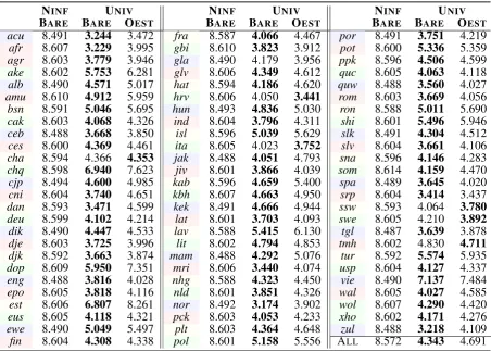
Table 1: BPC scores (lower is better) for the ZERO-SHOTlearning setting, with the uninformed prior (NINF) and the universal prior (UNIV): see§2for the descriptions of the priors. Note that for the former there is no difference between a BARE model and a conditional model (OEST). Colors define the split in which each language (rows) has been held out.
BARE OEST BARE OEST BARE OEST BARE OEST
acu 1.413 1.308 eng 1.355 1.350 kek 1.131 1.133 slk 1.844 1.754 afr 1.471 1.457 epo 1.471 1.450 lat 1.792 1.758 slv 1.848 1.793 agr 1.701 1.581 est 0.333 0.150 lav 2.146 1.931 sna 1.489 1.457 ake 1.453 1.377 eus 1.763 1.635 lit 1.895 1.833 som 1.477 1.468 alb 1.590 1.552 ewe 2.084 1.944 mam 1.654 1.548 spa 1.559 1.525 amu 1.402 1.340 fin 1.716 1.680 mri 1.342 1.330 srp 1.832 1.756 bsn 1.232 1.172 fra 1.465 1.432 nhg 1.302 1.238 ssw 1.890 1.697 cak 1.281 1.221 gbi 1.398 1.331 nld 1.621 1.601 swe 1.619 1.595 ceb 1.193 1.185 gla 3.403 1.839 nor 1.623 1.590 tgl 1.221 1.210 ces 1.872 1.795 glv 1.932 1.644 pck 1.731 1.711 tmh 2.786 2.301 cha 1.934 1.790 hat 1.480 1.454 plt 1.296 1.286 tur 1.801 1.773 chq 1.265 1.220 hrv 2.059 1.974 pol 1.743 1.698 usp 1.290 1.214 cjp 1.706 1.565 hun 1.887 1.847 por 1.586 1.552 vie 1.648 1.637 cni 1.348 1.290 ind 1.356 1.336 pot 2.484 2.144 wal 1.561 1.457 dan 1.727 1.693 isl 1.845 1.808 ppk 1.538 1.439 wol 2.053 1.890 deu 1.532 1.512 ita 1.615 1.583 quc 1.393 1.291 xho 1.680 1.634 dik 1.979 1.835 jak 1.415 1.322 quw 1.498 1.418 zul 1.880 1.620 dje 1.570 1.550 jiv 1.705 1.572 rom 1.706 1.587 ALL 1.652 1.550 djk 1.515 1.435 kab 1.955 1.791 ron 1.572 1.537
dop 1.810 1.676 kbh 1.436 1.371 shi 2.057 1.903
[image:6.595.73.528.478.724.2]NINF FITU UNIV NINF FITU UNIV
BARE OEST BARE OEST BARE OEST BARE OEST
acu 4.203 2.117 2.551 2.136 kbh 4.644 2.362 2.434 2.288 afr 4.423 3.620 3.042 2.773 kek 4.613 2.809 3.015 2.714 agr 4.268 3.282 3.403 2.457 lat 4.239 4.342 3.416 3.202 ake 4.318 2.168 2.238 2.180 lav 4.765 2.867 3.842 2.917
alb 4.544 3.186 3.302 3.084 lit 4.769 3.752 3.592 3.668
amu 4.486 2.820 3.948 2.080 mam 4.525 2.274 2.873 2.363
bsn 4.546 1.861 2.678 1.850 mri 3.795 3.482 3.010 2.459 cak 4.426 1.994 2.053 1.956 nhg 4.373 2.004 2.480 1.965 ceb 4.084 2.562 2.595 2.470 nld 4.469 3.008 2.908 2.903 ces 4.984 4.651 4.190 3.680 nor 4.453 3.152 2.954 3.054
cha 4.329 2.546 2.899 2.525 pck 4.246 4.011 3.532 3.030 chq 4.941 1.948 2.078 1.963 plt 4.201 2.532 2.742 2.490 cjp 4.424 2.389 2.880 2.393 pol 4.853 3.852 3.620 3.788
cni 4.185 2.797 3.018 1.982 por 4.446 3.231 3.198 3.098 dan 4.719 3.211 3.127 3.180 pot 4.299 3.773 3.944 2.763 deu 4.589 3.103 3.007 2.953 ppk 4.439 2.220 2.736 2.236
dik 4.380 2.640 3.020 2.667 quc 4.538 2.154 2.242 2.108 dje 4.382 3.815 3.398 2.898 quw 4.223 2.196 2.547 2.158 djk 4.130 2.064 2.446 2.085 rom 4.378 3.121 3.257 2.455 dop 4.508 2.506 2.562 2.448 ron 4.579 3.273 3.734 3.216 eng 4.436 2.808 2.913 2.719 shi 4.509 2.963 3.092 2.970
epo 4.469 3.609 3.511 2.825 slk 4.873 3.722 3.812 3.631 est 3.618 1.952 2.487 1.962 slv 4.633 4.630 3.527 3.501 eus 4.354 2.628 2.705 2.567 sna 4.455 2.910 3.114 2.870 ewe 4.590 2.806 3.336 2.786 som 4.257 3.048 2.908 2.934
fin 4.385 4.339 3.830 3.312 spa 4.507 3.223 3.149 3.090 fra 4.551 3.086 3.276 2.981 srp 4.561 4.467 3.367 3.380
gbi 4.250 2.138 2.170 2.054 ssw 4.370 2.611 2.924 2.570 gla 4.159 2.377 2.835 2.395 swe 4.657 3.266 3.184 3.177 glv 4.346 3.523 3.702 2.644 tgl 4.060 2.546 2.592 2.436 hat 4.468 2.929 3.048 2.849 tmh 4.618 4.087 4.218 3.125 hrv 4.615 3.845 3.608 3.588 tur 4.846 3.509 4.282 3.552
hun 4.806 3.589 3.709 3.522 usp 4.529 2.114 2.189 2.073 ind 4.377 3.317 3.258 2.420 vie 5.185 3.018 3.751 3.015 isl 4.744 3.174 3.703 3.101 wal 4.398 2.986 3.623 2.278 ita 4.370 3.384 3.196 3.178 wol 4.621 2.898 2.968 2.826 jak 4.532 2.113 2.650 2.126 xho 4.561 3.415 3.208 3.289
[image:7.595.107.490.65.532.2]jiv 4.338 3.413 3.475 2.504 zul 4.564 2.625 2.866 2.622 kab 4.649 2.783 3.574 2.800 ALL 4.467 3.007 3.120 2.731
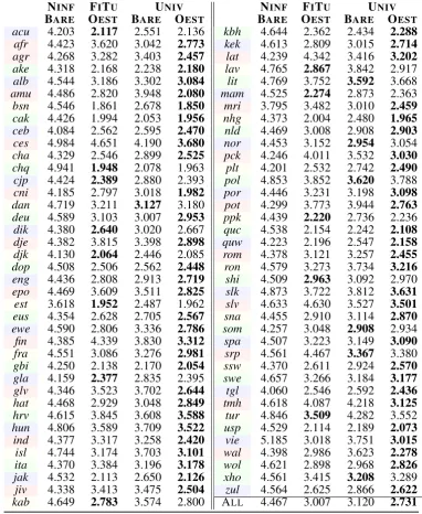
Table 3: BPC scores (lower is better) for the FEW-SHOT learning setting, with NINF, FITU and UNIVpriors. Colors define the split in which each language (rows) has been held out.
Language Model We implement the LSTM fol-lowing the best practices and hyper-parameter set-tings indicated for language modelling byMerity et al.(2017,2018). In particular, we optimize the weights with Adam (Kingma and Ba,2014) and a non-monotonically decayed learning rate: its value is initialized as10−4and decreases by a factor of 10 every1/3rd of the total epochs. The maximum number of epochs amounts to 6 forDt, with early stopping based on development set performance, and the maximum number of epochs is 25 forDe.
Moreover, we extend the model to multilingual joint training. In each iteration, we sample a
lan-guage proportionally to the amount of its data:
p(`)∝ |Dt|, in order not to exhaust examples from resource-lean languages in the early phase of train-ing. Then, we sample without replacement fromDt a mini-batch of 128 sequences with a variable max-imum sequence length.12 This length is sampled from a distributionm ∼ N(µ = 125, σ = 5).13 Each epoch comes to an end when all the data se-quences have been sampled.
We apply several techniques of dropout for
regu-12
This avoids creating insurmountable boundaries to back-propagation though time (Tallec and Ollivier,2017).
13The learning rate is therefore scaled bym µ and
larization, including variational dropout (Gal and Ghahramani, 2016), which applies an identical mask to all time steps, with p = 0.1for charac-ter embeddings and incharac-termediate hidden states and
p= 0.4for the output hidden states. DropConnect (Wan et al.,2013) is applied to the model parame-tersU of the first hidden layer withp= 0.2.
FollowingMerity et al.(2017), the underlying language model architecture consists of 3 hidden layers with 1,840 hidden units each. The dimen-sionality of the character embeddings is 400. For conditional language models, the dimensionality of
f(t)is set to 115 with theOESTmethod based on concatenation (Ostling and Tiedemann,¨ 2017), and 4 (due to memory limitations) in thePLATmethod
based on meta-networks (Platanios et al., 2018). For the regularizer in eq. (17), we perform grid search over the hyperparameterλ: we finally select a value of105for UNIVand10−5for NINF.
Regimes of Data Paucity We explore different regimes of data paucity for the held-out languages: •ZERO-SHOTtransfer setting: we split the sample of 77 languages into 4 subsets. The languages in each subset are held out in turn, and we use their test set for evaluation.14For each subset, we further randomly choose 5 languages whose development set is used for validation. The training set of the rest of the languages is used to estimate a prior over network parameters via the Laplace approximation. •FEW-SHOTtransfer setting: on top of the zero-shot setting, we use the prior to perform MAP in-ference over a small sample (100 sentences) from the training set of each held-out language.
•JOINTmultilingual setting:Deincludes the full training set for all 77 languages, including held-out languages. This works as a ceiling for the expected performance of language transfer models.
6 Results and Analysis
The results for our experiments are grouped in Ta-ble1for the ZERO-SHOTregime, Table3for the
FEW-SHOTregime, and in Table2for the JOINT
multilingual regime. The scores represent Bits Per Character (BPC) (Graves,2013): this metric is sim-ply defined as the average negative log-likelihood of test data divided bylog 2. We compare the re-sults along the following dimensions:
14Holding out each language individually would not in-crease the sample of training languages significantly, while inflating the number of experimental runs needed.
Informativeness of Prior Our main result is that the UNIVprior consistently outperforms the NINF
prior across the board and by a large margin in both
ZERO-SHOTandFEW-SHOTsettings. The scores for the na¨ıvest baseline, ZERO-SHOTNINFBARE, are considerably worse than with both ZERO-SHOT
UNIV models: this suggests that the transfer of
information on character sequences is meaningful. The lowest BPC reductions are observed for lan-guages like Vietnamese (15.94% error reduction) or Highland Chinantec (19.28%) where character inventories or distributions are unmatched in other languages. Moreover, the ZERO-SHOTUNIV
mod-els are on a par or better than even the FEW-SHOT
NINFmodels. In other words, the most helpful su-pervision comes from a universal prior rather than from a small in-language sample of sentences. This demonstrates that the UNIVprior is truly imbued with universal linguistic knowledge that facilitates learning of previously unseen languages.
The averaged BPC score for the other baseline without a prior, FINE-TUNEis 3.007 for FEW-SHOT
OEST, to be compared with 2.731 BPC of UNIV. Note that fine-tuning is an extremely competitive baseline, as it lies at the core of most state-of-the-art NLP models (Peters et al.,2019). Hence, this result demonstrates the usefulness of a Bayesian treatment of transfer learning.
Conditioning on Typological Information An-other important result regards the fact that condi-tioning language models on typological features yield opposite effects in theZERO-SHOTandFEW
-SHOTsettings. By comparing the BAREand OEST
models’ columns in Table1, the non-conditional baseline BARE is superior for 71 / 77 languages (the exceptions being Chamorro, Croatian, Italian, Swazi, Swedish, and Tuareg). On the other hand, the same columns in Table3 and Table2 reveal an opposite pattern: OESToutperforms the BARE
baseline in 70 / 77 languages. Finally, OEST sur-passes the BAREbaseline in the JOINTsetting for 76 / 77 languages (save Q’eqchi’).
We also also take into consideration an alter-native conditioning method, namely PLAT. For clarity’s sake, we exclude this batch of results from Table1and Table3, as this method proves to be consistently worse than OEST. In fact, the average BPC of PLATamounts to 5.479 in the ZERO-SHOT
The possible explanation behind the mixed evi-dence on the success of typological features points to some intrinsic flaws of typological databases. Ponti et al.(2018a) has shown how their feature granularity may be too coarse to be reconciled with data-driven probabilistic models, and their limited coverage of features introduces noise as missing values have to be inferred. As a result, language models seem to be damaged by typological fea-tures in absence of data, whereas they find a way to follow their guidance when at least a small sample of sentences is available in the FEW-SHOTsetting.
Data Paucity Different regimes of data paucity display uneven levels of performance. The best models for each setting (ZERO-SHOT UNIV BARE,
FEW-SHOTUNIVOEST, and JOINTOEST) reveal large gaps between their average scores. Hence, in-language supervision should be still considered unsubstitutable, and transferred language models still lag behind their resource-rich equivalents.
7 Related Work
LSTMs have been probed for an inductive bias in capturing syntactic dependencies (Linzen et al., 2016) and grammaticality judgements (Marvin and Linzen,2018;Warstadt et al.,2018).Ravfogel et al. (2019) have extended the scope of this analysis to typologically different languages throughsynthetic
variations of English. In this work, we aim to model the inductive bias explicitly by constructing a prior over the space of neural network parameters.
Few-shot word-level language modelling for truly under-resourced languages such as Yongning Na has been investigated byAdams et al.(2017) with the aid of a bilingual lexicon. Vinyals et al. (2016) andMunkhdalai and Trischler(2018) pro-posed novel architectures (Matching Networks and LSTMs augmented with Hebbian Fast Weights, re-spectively) for rapid associative learning in English, and evaluated them in few-shot cloze tests. In this respect, our work is novel in pushing the problem to its most complex formulation, zero-shot infer-ence, and in taking into account the largest sample of languages for language modelling to date.
In addition to the set of standard architectures considered in our work, there are also alternatives to conditional language modelling. Kalchbren-ner and Blunsom (2013) used encoded features as additional biases in recurrent layers.Kiros et al. (2014) put forth a log-bilinear model that allows for a “multiplicative interaction” between hidden
representations and input features (such as images). With a similar device, but a different gating method, Tsvetkov et al.(2016) trained a phoneme-level joint multilingual model of words conditioned on typo-logical features fromMoran et al.(2014).
The use of the Laplace method for neural trans-fer learning has been proposed byKirkpatrick et al. (2017), inspired by synaptic consolidation in neuro-science to avoid catastrophic forgetting.Kochurov et al. (2018) tackled the problem of continuous learning from independent data portions for a single fixed task by approximating the posterior probabili-ties through stochastic variational inference.Ritter et al.(2018) substitute diagonal Laplace approxima-tion with a Kronecker factored method, leading to better uncertainty estimates. Finally, the regularizer proposed byDuong et al.(2015) for cross-lingual dependency parsing can be interpreted as a prior for Maximum A Posteriori estimation where the covariance is an identity matrix.
8 Conclusions
In this work, we proposed a Bayesian approach to cross-lingual language modeling transfer. We created a universal prior over neural network weights that is capable of generalizing well to new languages riddled by data paucity, by Laplace-approximating the posterior of the weights condi-tioned on the data from a sample of training lan-guages. Based on the results of character-level language modelling on a sample of 77 languages, we demonstrated the superiority of the universal prior over uninformative priors and uniform pri-ors (i.e., the widespread fine-tuning approach) in both zero-shot and few-shot settings. Moreover, we showed that adding language-specific side in-formation drawn from typological databases to the universal prior further increases the levels of per-formance in the few-shot regime. While we also showed that language transfer still lags behind mul-tilingual joint learning when sufficient in-language data are available, our work is the first step towards bridging this gap in the future.
Acknowledgements
References
Oliver Adams, Adam Makarucha, Graham Neubig, Steven Bird, and Trevor Cohn. 2017. Cross-lingual word embeddings for low-resource language model-ing. InProceedings of EACL, pages 937–947.
Adriano Azevedo-Filho and Ross D. Shachter. 1994.
Laplace’s method approximations for probabilistic inference in belief networks with continuous vari-ables. InProceedings of UAI, pages 28–36.
Cecil H. Brown, Eric W. Holman, Søren Wichmann, and Viveka Velupillai. 2008. Automated classifica-tion of the world’s languages: A descripclassifica-tion of the method and preliminary results. STUF-Language Typology and Universals Sprachtypologie und Uni-versalienforschung, 61(4):285–308.
Noam Chomsky. 1959. A review of BF Skinner’s ver-bal behavior.Language, 35(1):26–58.
Noam Chomsky. 1978. A naturalistic approach to lan-guage and cognition. Cognition and Brain Theory, 4(1):3–22.
Christos Christodouloupoulos and Mark Steedman. 2015. A massively parallel corpus: The Bible in 100 languages. Language Resources and Evalua-tion, 49(2):375–395.
Chris Collins and Richard Kayne. 2009. Syntactic structures of the world’s languages. http://
sswl.railsplayground.net/.
Ryan Cotterell, Sebastian J. Mielke, Jason Eisner, and Brian Roark. 2018. Are all languages equally hard to language-model? InProceedings of NAACL-HLT, pages 536–541.
Thomas M. Cover and Joy A. Thomas. 2006. Elements of Information Theory. Wiley-Interscience.
William Croft. 2002. Typology and Universals. Cam-bridge University Press.
William Croft, Dawn Nordquist, Katherine Looney, and Michael Regan. 2017. Linguistic typology meets Universal Dependencies. InProceedings of TLT, pages 63–75.
Matthew S. Dryer and Martin Haspelmath, editors. 2013. WALS Online. Max Planck Institute for Evo-lutionary Anthropology.
Long Duong, Trevor Cohn, Steven Bird, and Paul Cook. 2015. Low resource dependency parsing: Cross-lingual parameter sharing in a neural network parser. InProceedings of ACL, pages 845–850.
Nicholas Evans and Stephen C. Levinson. 2009. The myth of language universals: Language diversity and its importance for cognitive science.Behavioral and Brain Sciences, 32(5):429–448.
Yarin Gal and Zoubin Ghahramani. 2016. A theoret-ically grounded application of dropout in recurrent neural networks. InProceedings of NeurIPS, pages 1019–1027.
Andrew Gelman, Hal S. Stern, John B. Carlin, David B. Dunson, Aki Vehtari, and Donald B. Rubin. 2013. Bayesian data analysis. Chapman and Hall/CRC.
Daniela Gerz, Ivan Vuli´c, Edoardo Ponti, Jason Narad-owsky, Roi Reichart, and Anna Korhonen. 2018a.
Language modeling for morphologically rich lan-guages: Character-aware modeling for word-level prediction. Transactions of the Association of Com-putational Linguistics, 6:451–465.
Daniela Gerz, Ivan Vuli´c, Edoardo Maria Ponti, Roi Reichart, and Anna Korhonen. 2018b. On the rela-tion between linguistic typology and (limitarela-tions of) multilingual language modeling. InProceedings of EMNLP, pages 316–327.
Gary Martin Gilligan. 1989. A cross-linguistic ap-proach to the pro-drop parameter. Ph.D. thesis, Uni-versity of Southern California.
Giorgio Graffi. 1980. Universali di Greenberg e gram-matica generativa in la nozione di tipo e le sue arti-colazioni nelle discipline del linguaggio. Lingua e Stile Bologna, 15(3):371–387.
Alex Graves. 2013. Generating sequences with recur-rent neural networks.CoRR, abs/1308.0850.
Joseph H. Greenberg. 1963. Some universals of gram-mar with particular reference to the order of mean-ingful elements.Universals of Language, 2:73–113.
Sepp Hochreiter and J¨urgen Schmidhuber. 1997.
Long short-term memory. Neural Computation, 9(8):1735–1780.
Nal Kalchbrenner and Phil Blunsom. 2013. Recurrent continuous translation models. In Proceedings of EMNLP, pages 1700–1709.
Diederik P. Kingma and Jimmy Ba. 2014. Adam: A method for stochastic optimization. InProceedings of ICLR.
James Kirkpatrick, Razvan Pascanu, Neil Rabinowitz, Joel Veness, Guillaume Desjardins, Andrei A Rusu, Kieran Milan, John Quan, Tiago Ramalho, Ag-nieszka Grabska-Barwinska, et al. 2017. Over-coming catastrophic forgetting in neural networks. Proceedings of the National Academy of Sciences, 114(13):3521–3526.
Ryan Kiros, Ruslan Salakhutdinov, and Rich Zemel. 2014. Multimodal neural language models. In Pro-ceedings of ICML, pages 595–603.
Andr´as Kornai. 2013. Digital language death. PloS One, 8(10):e77056.
Julie Anne Legate and Charles D Yang. 2002. Em-pirical re-assessment of stimulus poverty arguments. The Linguistic Review, 18(1-2):151–162.
Tal Linzen, Emmanuel Dupoux, and Yoav Goldberg. 2016. Assessing the ability of LSTMs to learn syntax-sensitive dependencies. Transactions of the Association for Computational Linguistics, 4:521– 535.
Patrick Littell, David R. Mortensen, Ke Lin, Kather-ine Kairis, Carlisle Turner, and Lori Levin. 2017.
URIEL and lang2vec: Representing languages as typological, geographical, and phylogenetic vectors. InProceedings of EACL, pages 8–14.
Rebecca Marvin and Tal Linzen. 2018. Targeted syn-tactic evaluation of language models. In Proceed-ings of EMNLP, pages 1192–1202.
Stephen Merity, Nitish Shirish Keskar, and Richard Socher. 2017. Regularizing and optimizing LSTM language models.arXiv preprint arXiv:1708.02182.
Stephen Merity, Nitish Shirish Keskar, and Richard Socher. 2018. An analysis of neural language modeling at multiple scales. arXiv preprint arXiv:1803.08240.
Sebastian J. Mielke, Ryan Cotterell, Kyle Gorman, Brian Roark, and Jason Eisner. 2019. What kind of language is hard to language-model? In Proceed-ings of ACL, pages 4975–4989.
Steven Moran, Daniel McCloy, and Richard Wright, ed-itors. 2014. PHOIBLE Online. Max Planck Institute for Evolutionary Anthropology, Leipzig.
Tsendsuren Munkhdalai and Adam Trischler. 2018.
Metalearning with Hebbian fast weights. arXiv preprint arXiv:1807.05076.
Robert ¨Ostling and J¨org Tiedemann. 2017.Continuous multilinguality with language vectors. In Proceed-ings of the EACL, volume 2, pages 644–649.
Razvan Pascanu, Tomas Mikolov, and Yoshua Bengio. 2013. On the difficulty of training recurrent neu-ral networks. InProceedings of ICML, pages 1310– 1318.
Matthew Peters, Sebastian Ruder, and Noah A Smith. 2019. To tune or not to tune? adapting pretrained representations to diverse tasks. arXiv preprint arXiv:1903.05987.
Emmanouil Antonios Platanios, Mrinmaya Sachan, Graham Neubig, and Tom Mitchell. 2018. Contex-tual parameter generation for universal neural ma-chine translation. InProceedings of EMNLP, pages 425–435.
Edoardo Maria Ponti, Helen O’Horan, Yevgeni Berzak, Ivan Vuli´c, Roi Reichart, Thierry Poibeau, Ekaterina Shutova, and Anna Korhonen. 2018a. Modeling lan-guage variation and universals: A survey on typo-logical linguistics for natural language processing. arXiv preprint arXiv:1807.00914.
Edoardo Maria Ponti, Roi Reichart, Anna Korhonen, and Ivan Vuli´c. 2018b. Isomorphic transfer of syn-tactic structures in cross-lingual NLP. In Proceed-ings of ACL, pages 1531–1542.
Shauli Ravfogel, Yoav Goldberg, and Tal Linzen. 2019.
Studying the inductive biases of RNNs with syn-thetic variations of natural languages. In Proceed-ings of NAACL-HLT.
Shauli Ravfogel, Yoav Goldberg, and Francis Tyers. 2018. Can LSTM learn to capture agreement? The case of Basque. InProceedings of the 2018 EMNLP Workshop BlackboxNLP: Analyzing and Interpreting Neural Networks for NLP, pages 98–107.
Hippolyt Ritter, Aleksandar Botev, and David Barber. 2018.Online structured Laplace approximations for overcoming catastrophic forgetting. InProceedings of NIPS, pages 3738–3748.
Sebastian Ruder. 2017. An overview of multi-task learning in deep neural networks. arXiv preprint arXiv:1706.05098.
Gary F. Simons. 2017. Ethnologue: Languages of the world, 22nd edition. Dallas, Texas: SIL Interna-tional.
Ilya Sutskever, Oriol Vinyals, and Quoc V Le. 2014.
Sequence to sequence learning with neural networks. InProceedings of NIPS, pages 3104–3112.
Corentin Tallec and Yann Ollivier. 2017. Unbias-ing truncated backpropagation through time. arXiv preprint arXiv:1705.08209.
Yulia Tsvetkov, Sunayana Sitaram, Manaal Faruqui, Guillaume Lample, Patrick Littell, David Mortensen, Alan W. Black, Lori Levin, and Chris Dyer. 2016. Polyglot neural language models: A case study in cross-lingual phonetic represen-tation learning. In Proceedings of NAACL-HLT, pages 1357–1366.
Oriol Vinyals, Charles Blundell, Timothy Lillicrap, Daan Wierstra, et al. 2016. Matching networks for one shot learning. In Proceedings of NIPS, pages 3630–3638.
Li Wan, Matthew Zeiler, Sixin Zhang, Yann Le Cun, and Rob Fergus. 2013. Regularization of neural net-works using DropConnect. InProceedings of ICML, pages 1058–1066.