Abstract—Online auctions have expanded rapidly over the decade and had turn to a fascinating new type of business or commercial transaction in the digital era. Bidding in an online auction is a very challenging task as the bidder is not acquainted with the amount, time and also venue. The bidders will end up winning or losing in an auction. One of the ways to ensure a winning bid is for the bidder to try and predict the closing price of a given auction. However, it is not easy to predict the closing price of an auction since it depends on several factors such as the amount of identical auctions running, the amount of participants as well as the behaviour of every individual bidder. On top of this, there can be multiple auctions running concurrently at the same time that can influence the auctions results. This paper discussed on the prediction of online auction closing price using two well known theories which are the Grey Theory (GT) and the Artificial Neural Network (ANN) – Backpropagation (BP). The prediction, accuracy and effectiveness for both models will be evaluated using a simulated auction environment.
I. INTRODUCTION
UCTION is a market institution with an explicit set of rules determining resource allocation and price on the basis of bid from the market participants [16]. Auction mechanisms have become very popular within electronic commerce and have been implemented in many domains with assorted environments. Unlike traditional auction houses, online auction websites offers a better place for people to purchase and publicize merchandise through a bidding process. Online auction has given consumers a “virtual” flea market with all the new and used merchandises from around the world. They also give sellers a global storefront where they are able to market their goods.
Online auctions provide many benefits compared to the traditional auctions. One disadvantage of having traditional auction is that it requires simultaneous participation of all bidders or agents at the same location. In online auction, this does not exist as online auction allows clients to make their purchases anywhere anytime. Online auctions also provide bidders more flexibility on when to submit their bids since online auctions usually last for days or even weeks. Compared to the traditional business type, internet auctions can be a co-effective way on testing on the product markets and are able to liquidate dated or overstocked merchandise especially for small business owners. Besides that, online auction can be more effective as the target audiences will be in a mass amount where there is no geographical limitation
since both sellers and buyers do their trading in a “virtual” environment and any payment transaction can be made through the online banking. Having a relative low price and wider market in products and services, it had made the online auction a success where it attracts many bidders and also sellers as well. Online auctions also allow sellers to sell their goods efficiently and with little exertion required.
The demands for online auction are increasing. Some examples of popular online auction houses include eBay, Amazon, Yahoo!Auction, Priceline, UBid, and FirstAuction. EBay is the world’s online marketplace, where the buyers and sellers come together and trade almost anything. Most of the auctions in eBay are based on English auction constrained by time. The English auction begins with the lowest price and bidders are free to raise their bid successively until there are no more offers to raise the bid and the bidder with the highest bid will be the winner [11]. If there are no bidders at the end of the auction or the current highest bid is lower than the seller’s reserve price, then the auction will close without a winner. E-Bay also allow sellers to set a reasonable price on the item being sold so that consumers can directly purchase without bidding.
Due to the proliferation of these online auctions, consumers are faced with the problem of monitoring multiple auction houses, picking which auction to participate in, and making the right bid to ensure that they get the item under conditions that are consistent with their preferences[2].These processes of monitoring, selecting and making bids are time consuming. The task becomes even more challenging when the individual auctions have different start and end times. Moreover, auctions can last for a few days or even weeks. Besides that, every bidder has his own reservation price or maximum amount that he is willing to bid for each item. If bidders are able to predict the closing price for each auction then they are able to make a better decision on the time, place and the amount they can bid for an item. In a situation where a bidder has to decide among the many auctions that are currently ongoing, this knowledge on closing price for an auction would be useful for the bidder to decide on which auction to participate, when to participate and at what price. There are other considerations that need to be taken into account to ensure that the bidder wins in a given auction. For example, in eBay, any bidder who wishes to participate in an online auction does not have any information on how many bidders will bid in the auction, the number of bids and how the auction will progress over time.
However, having a good prediction on the closing price of a given auction would definitely be an advantage as the bidder
Assessing the Accuracy of Grey System Theory against
Artificial Neural Network in Predicting Online Auction
Closing Price
Deborah Lim, Patricia Anthony, Ho Chong Mun, and Ng Kah Wai
can decide the amount and time to bid. Besides that it would be a lot easier for bidders if they can guess the price of the auction, so that they only need to bid at the last minutes of the auction. Unfortunately, predicting a closing price for an auction is not easy since it is dependent on many factors such as the behaviour and the number of the bidders who are participating in that auction.
Having many obstacles in bidding, many investors have been trying to find a better way to predict auction closing price accurately. Neural Network, Fuzzy Logic, Evolutionary Computation, Probability Function and Genetic Algorithm, are integrated to become more commendable practical model for prediction purpose. A large body of analysis techniques has been developed, particularly from methods in statistics and signal processing. The most popular method is Artificial Neural Network (ANN), began approximately fifty years ago, where it is based on computer algorithms that attempt to simulate the parallel, highly interactive distributed processing in brain tissue. As being acknowledged, forecasting or prediction needs a lot of historical data. ANN has been successfully applied to a wide variety of problems, such as storing and recalling data or patterns, classifying patterns, performing general mapping from input patterns to output patterns, grouping similar patterns, or finding solutions to constrained optimization problems [12]. One other method is the Grey Theory. It is a new theory and method which applies to the study of unascertained problems with few or poor incoming information [13]. It has been successfully applied to economical, management, social systems, industrial systems, ecological systems, education, traffic, environmental sciences, and geography [14].
In our previous work we evaluated the effectiveness of the Grey Theory model, against the performance the Simple Exponential Function and ARIMA Time Series [6]. We also set up an electronic simulated marketplace to simulate the real online auctions environment. In this particular work we found that the Grey System Theory gives higher accuracy in predicting the online auction closing price [1], [6], [7]. However, we did not apply the model to a real auction data such as eBay. Hence, in this work, we will investigate the performance of the Grey Theory Model and the Simple Exponential Function in a real online auction setting.
There are many researches that have been engaging in the prediction and forecasting of real world phenomenon. Chen et al. [3] proposed a model to forecast Li-ion battery charge by using grey theory. Lin and Lin [15] used grey prediction to improve the efficiency of achieving accurate and speedy inspection when a coordinate measuring machine (CMM) is used to measure circularity geometric tolerance. Baokui et al. [21] applied grey theory to predict the gas-in-oil concentrations in oil-filled transformer. The gas-in-oil concentrations are used to diagnose oil-filled transformer insulation. Taylor and Buizza [20] have investigates the use of weather ensemble predictions in the application of ANNs to load forecasting for lead times from one to ten days ahead. Nogueira et al. [17] propose a new modeling approach, based on neural networks, that is able to predict the Quality of Service (QoS) of wireless local area networks (WLANs) based on the characterization of an operational scenario.
In this paper, we will investigate and compare the
effectiveness of the Grey Theory and Artificial Neural Network in predicting the closing price of online auction. In Section II, the design of Grey Theory is explained. Section III discusses the prediction algorithm using the Grey Theory. Section IV elaborates the design of Artificial Neural Network and Backpropagation Prediction Algorithm in section V. The experimental results are shown in Section VI. Section VII discussed some related works using Grey Theory and Artificial Neural Network and finally the conclusion and future work is discussed in Section VIII.
III. GREY SYSTEM THEORY
The Grey System Theory was first proposed by Deng Julong (1982) [8], where this theory works on unascertained systems with partially known and partially unknown information by drawing out valuable information and also by generating and developing the partially known information. It can describe correctly and monitor effectively the systemic operational behaviour [13]. Basically, the Grey System Theory was chosen based on color [14]. For instance, “black” is used to represent unknown information and “white” is the colour used for complete information. Those partially know and partially unknown information is called the “Grey System Theory”.
TABLE I
ATTRIBUTES OF TRADITIONAL FORECASTING MODEL Mathematical model Minimum observation Type of sample Sample interval Mathematical requirements Simple Exponential Function
5-10 Interval Short Basic
Regression Analysis
10-20 Trend Short Middle
Casual Regression
10 Any
type
Long Advanced
Box-Jenkins 50 Interval Long Advanced
Neural Network Large number
Interval or not
Short Advanced
Grey Prediction Model
4 Interval Long Basic
Grey prediction is a quantitative prediction based on Grey Generating Function, GM (1,l) Model, which uses the variation within the system to find the relations between sequential data and then establish the prediction model. The Grey Forecasting Model is derived from the Grey System, in which one examines changes within a system to discover a relation between sequence and data. After that, a valid prediction is made to the system. Grey Prediction Model has the following advantages: (a) It can be used in situations with relatively limited data down to as little as four observations, as stated in TABLE I. (b) A few discrete data are sufficient to characterize an unknown system. (c) It is suitable for forecasting in competitive environments where decision makers have only accessed to limited historical data [5].
IV. GREY THEORY PREDICTION ALGORITHM
In this section we focus on the Grey Generating Function, GM (1,1) which are being used in grey prediction [9,14]. The algorithm of GM (1,1) can be summarized as follows. Step 1. Establish the initial sequence from observation data. In this case, the data used is the previous values of the online auction closing price observed over time.
. 2 where }, ,..., , ,
{ 0 0
3 0 2 0 1
0= ≥
n f f f f f n
Step 2. Generate the first-order accumulated generating operation (AGO) sequence
∑
= = = = t k k tn f f and t n
f f f f f 1 0 1 1 1 3 1 2 1 1 1 . ,..., 2 , 1 where }, ,..., , , {
Step 3. The grey model GM (1,1)
( ) , 1.
2
1 1 1
1 0
1 + ∀ ≥
− +
= +
+ a f f b t
ft t t
Step 4. Rewrite into matrix form
( ) ( ) ( ) . 1 2 1 1 2 1 1 2 1 1 1 1 1 2 1 3 1 1 1 2 0 0 3 0 2 + − + − + − = − b a f f f f f f f f f n n n M M M
Step 5. Solve the parameter a and b
(
)
(
)
(
)
(
)
+ − + − + − = = = + − 1 2 1 1 2 1 1 2 1 and where , 1 1 1 2 1 3 1 1 1 2 0 0 3 0 2 0 0 1 n n n T T f f f f f f B f f f F F B B B b a M M MStep 6. Estimate AGO value
. 1 , ˆ 0 1 1
1 ∀ ≥
+ − = − + t a b e a b f f at t
Step 7. Get the estimate IAGO value or the estimated closing price for a given auction.
2. t , ˆ ˆ ˆ 1 1 1
0= − ∀ ≥
−
t t t f f
f
Step 8. We use the average residual error for each set of data to calculate the accuracy of the predicted data. The formula for the average residual error (ARE) is given as
%, 100 1 1 0 0 0 × −
∑
= n t t t t f f f n )Where 0=real valueofexchangerateat time t
t
f
ˆ0=estimated valueofexchangerateat time t
t f n observatio total = n
V. ARTIFICIAL NEURAL NETWORK DESIGN
An Artificial Neural Network (ANN) is an information processing paradigm that is inspired by biological nervous systems, such as the brain, process information [12]. A Neural Network one of the most powerful data modeling tool that is able to capture and represent complex input and output relationships. Neural Networks are composed of simple elements operating in parallel. These elements are inspired by biological nervous systems. As in nature, the network function is determined largely by the connections between elements. We can train a Neural Network to perform a particular function by adjusting the values of the connections (weights) between elements.
The first fundamental modeling of Neural Nets was proposed in 1943 by McCulloch and Pitts in their classic paper that gave to the notion of a “Boolean brain” [18]. As in nature, a Neural Net consists of a large number of simple processing element called neurons, units, cells, or notes. Each neuron is connected to other neurons by means of directed communication links, each with an associated weight. The weight represents information being used by the net to solve a problem. By its learning algorithm to adjust weighted connections between Artificial Neurons, ANN is able to be "trained" to conduct specific tasks. When an ANN commits an error, this error is being calculated and the weights of connections are adjusted [10].
Commonly Neural Networks are adjusted, or trained, so that a particular input leads to a specific target output. There, the network is adjusted, based on a comparison of the output and the target, until the network output matches the target. Typically many such input/target pairs are needed to train a network
Neural Networks can be applied to a wide variety of problems, such as storing and recalling data or patterns, classifying patterns, performing general mapping from input patterns to output patterns, grouping similar patterns, or finding solutions to constrained optimizations problems [12]. Neural Network is typically organized in layer where the layers made up of a number of interconnected 'nodes' which contain an 'activation function'. Patterns are presented to the network via the 'input layer', which communicates to one or more 'hidden layers' where the actual processing is done via a system of weighted 'connections'. The hidden layers then link to an 'output layer' where the answer is output. Commonly Neural Networks are adjusted, or trained, so most ANN contains some form of 'learning rule' which modifies the weights of the connections according to the input patterns that it is presented with. ANN therefore learns by example as do their biological counterparts; a child learns to recognize dogs from examples of dogs[12].
VI. BACKPROPAGATION PREDICTION ALGORITHM
The Standard Backpropagation algorithm is shown as follow [12]:
Step 0. Initialize weights.
Set to small random values.
Step 1. While stopping condition is false, do Steps 2 to 9. Step 2. For each training pair, do Steps 3 to 8.
Feedforward:
Step 3. Each input unit (Xi, i = 1, …, n) receives input
signal xi and broadcasts this signal to all units in
the layer above (the hidden units).
Step 4. Each Hidden unit (Zj, j = 1, …, p) sums its weight
input signals, z_inj = v0j + ij
n
i iv x
∑
=1
, applies its
activation function to compute its output signal, zj
= f (z_inj), and sends this signal to all units in the
layer above (output units).
Step 5. Each output unit (Yk, k = 1, …, m) sums its
weighted input signals, y_ink = w0k +
jk p
j jw
z
∑
=1 and applies its activation function to compute its output signal, yk = f (y_ink).
Backpropagation of error:
Step 6. Each output unit (Yk, k = 1, …, m) receives a
target pattern corresponding to the input training pattern, computes its error information term,
) _ ( )
( '
k k
k
k = t −y f y in
δ , calculates its weight
correction term (used to update wjk later),
j k
jk z
w =αδ
∆ , calculate its bias correction term (used to update w0k later), ∆w0k =αδk, and sends
k
δ
to units in the layer below.Step 7. Each hidden unit (Zj, j = 1, …, p) sums its delta
inputs (from unit in the later above),
jk m
k k
j w
in
∑
= =
1
_ δ
δ , multiplies by the derivative of its
activation function to calculate its error information term, δ =j δ_injf'(z_inj), calculate
its weight correction term (used to update vij later,
i j
ij x
v =αδ
∆ , and calculate its bias correction term (used to update v0j later), ∆v0ij =αδj.
Update weights and biases:
Step 8. Each output unit (Yk, k = 1, …, m) updates its bias
and weight (j = 0,..,p):
jk jk
jk new w old w
w ( )= ( )+∆ . Each hidden unit (Zj,
j = 1, …, p) updates its bias and weights (i = 1,…,n): vij(new)=vij(old)+∆vij.
Step 9. Test stopping condition.
Step 10. We use the average residual error (ARE) to calculate the accuracy of the predicted data.
%, 100 1
1 0
0 0
×
−
∑
= nt t
t t
f f f
n
)
Where 0=real valueofexchangerateat time t
t
f
t at time rate exchange of value estimated ˆ0=
t
f
n observatio total
= n
VII. PRELIMINARY EXPERIMENTAL EVALUATION
The purpose of this experimental evaluation is to determine the efficiency and accuracy of the Grey Prediction Model and Backpropagation Prediction Model in predicting the closing price of online auction. To calculate the prediction accuracy of this model, we worked on the original data taken from eBay Apple IPhone 8GB for Nov 2007 [22]. The closing price histories for all auctions running in a marketplace are shown from 1st November 2007 until 30th November 2007. We arrange the auction according to the closing price period which we set as t = 1 until t = 70, t is the closing time sequence of each auction.
Firstly, we will calculate the result by using fixed historical data for the Grey Prediction Model and we will do the same using the Backpropagation Prediction Model. In the second stage of the experiment, we use moving data rather than just fixed data for both models. Moving data in this respect means taking into account all the auctions that are closed at every time step.
TABLE II
RESULT PERFORMED BY USING GREY PREDICTION MODEL COMPARED WITH ORIGINAL DATA GENERATED BY AGENT
AUCTION
No of Histo-rical Data
Time t = 51, Original
Data = 500
Time t = 52, Original
Data = 495
Time t = 53, Original
Data = 535
Time t = 54, Original
Data = 535
Time t = 55, Original
Data = 500
ARE (%)
4 515.24 492.75 498.01 426.62 339.15 12.57
5 516.86 516.88 505.48 438.18 355.51 12.06
6 528.54 545.33 555.57 514.52 462.43 6.21
7 536.57 564.50 588.88 564.87 532.59 8.71
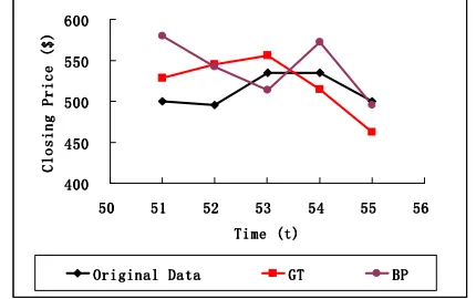
We also calculated the predicted closing price of online auction by using Backpropagation Prediction Model. Here, we predicted five future data of the auction closing price based on fifty historical data, one hidden layer containing fifteen neurons using different function (such as Tansig, and Logsig) and one output layer containing one neuron that use different function (such as Tansig, Logsig and Purelin). The result is shown in Table III. It can be seen that the average residual error (ARE) falls between 7.54% to 9.73%. In this case, the highest accuracy is both using Tansig with average residual error of 7.54%.
TABLE III
RESULT PERFORMED BY USING BACKPROPAGATION PREDICTION MODEL COMPARED WITH ORIGINAL DATA
GENERATED BY AGENT AUCTION Function
Type
Time t = 51, Original
Data = 500
Time t = 52, Original
Data = 495
Time t = 53, Original
Data = 535
Time t = 54, Original
Data = 535
Time t = 55, Original
Data = 500
ARE (%)
Tansig 580.00 542.53 513.38 572.84 495.03 7.54
Logsig 555.02 555.01 555.00 555.03 555.01 8.32
Logsis & Purelin
532.58 540.12 531.27 587.04 551.81 8.48
Tansig & Puelin
577.23 513.80 558.61 620.76 544.87 9.73
Based on these results, we can conclude that Grey Prediction Model, that used six historical data produced better result (ARE = 6.21%) than Backpropagation Prediction Model with Tansig function (ARE = 7.54%). Even with six historical data, Grey Theory is able to predict more accurately the closing price of the auctions in our simulated auction environment. Figure 2 show how that far off the two predictions against the actual closing price.
400 400400 400 450 450450 450 500 500500 500 550 550550 550 600 600600 600
50 50 50
50 51515151 52525252 53535353 54545454 55555555 56565656 Time (t)
Time (t)Time (t) Time (t)
C
l
o
s
i
n
g
P
r
i
c
e
(
$
)
C
l
o
s
i
n
g
P
r
i
c
e
(
$
)
C
l
o
s
i
n
g
P
r
i
c
e
(
$
)
C
l
o
s
i
n
g
P
r
i
c
e
(
$
)
Original Data Original Data Original Data
Original Data GTGTGTGT BPBPBPBP
Fig. 2 Result Performed by using Backpropagation (BP) Prediction Model with Tansig Function and Grey Theory (GT) Prediction Model (6 Historical
Data) Compared with Original Data Generated by Agent Auction
As mentioned earlier, at every time steps, there are auctions that will be closing. This simply means that, if one wants to predict the future five data, one has to take into account the auctions that will be closing between the current time and the
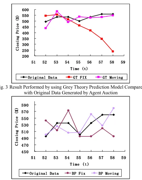
next time steps. Hence, we performed the following experiments in which we compared the result produced by six moving historical data with six fixed historical data using Grey Prediction Model and also fifty fixed historical data with fifty moving historical data by using Tansig Function for Backpropagation Prediction Model. TABLE IV shows the result obtained by using Grey Prediction Model and Backpropagation Prediction Model compared with the original data generated by EBay. The value on the right hand side box is the ARE ranking of GT, moving GT, BP and moving BP. By using ARE ranking value, we can clearly see the sequence of each predicted value by for different models. Table IV shows the Grey Prediction Model predicted values using this approach. In this particular experiment, the average residual error (ARE) of six fixed historical data is smaller than using six moving historical data when we predict the first three future data (52 – 54). However, when we moved down the predicted value (55 - 58), we can see that the prediction using six moving historical data is more accurate than using six fixed historical data. The differences between their ARE values for predicting four or more data are relatively bigger than the differences of ARE values for predicting the first three future data.
We then applied the same concept to the Backpropagation Prediction Model by comparing the predicted values using fifty fixed historical data and fifty moving historical data with Tansig Function. Table IV shows the predicted values for the two data groups. Figure 3 and Figure 4 shows the predicted values plotted against the actual closing prices for Grey Prediction Model and Backpropagation Prediction Model.
[image:5.595.58.273.547.682.2]In this particular experiment, the moving historical data performed better than the fixed historical data for both methods as can be seen in Figure 3 and Figure 4. The overall, Grey Prediction Model is still better than the Backpropagation Prediction Model based on moving historical data. However, using fixed historical data, the accuracy of Grey Prediction Model registered a higher ARE than the Backpropagation Prediction Model.
TABLE IV
RESULT OBTAINED BY USING GREY PREDICTION MODEL AND BACKPROPAGATION PREDICTION MODEL COMPARED WITH
ORIGINAL DATA GENERATED BY AGENT AUCTION
Time (t)
Original Data
(GT) Forecast Using 6 Fixed Historical
Data (ARE %)
(GT) Forecast Using 6 Moving Historical
Data (ARE %)
(BP) Forecast Using 50
Fixed Historical
Data (ARE %)
(BP) Forecast Using 50 Moving Historical
Data (ARE %)
51 500 528.54
(5.71)
1 528.54
(5.71)
1 580
(16.00)
2 580.00
(16.00) 2
52 495 545.33
(10.17)
3 439.06
(11.30)
4 542.53
(9.60)
2 500.23
(1.06) 1
53 535 555.57
(3.84)
2 583.16
(9.00)
4 513.38
(4.04)
3 525.62
(1.75) 1
54 535 514.52
(3.83)
1 490.75
(8.27)
4 572.84
(7.07)
3 505.55
(5.50) 2
55 500 462.43
(7.51)
4 537.06
(7.41)
3 495.03
(0.99)
1 507.16
(1.43) 2
56 535 418.95
(21.69)
4 529.93
(0.95)
1 495.03
(7.47)
3 561.82
(5.01) 2
57 560 345.86
(38.24)
4 533.53
(4.73)
1 519.16
(7.29)
3 527.07
(5.88) 2
58 560 237.45
(57.60)
4 548.48
(2.06)
1 495.01
(11.61)
3 579.68
200 200 200 200 250 250 250 250 300 300 300 300 350 350 350 350 400 400 400 400 450 450 450 450 500 500 500 500 550 550 550 550 600 600 600 600
51 51 51
51 52525252 53535353 54545454 55555555 56565656 57575757 58585858 59595959 Time (t)
Time (t) Time (t) Time (t)
C
l
o
s
i
n
g
P
r
i
c
e
(
$
)
C
l
o
s
i
n
g
P
r
i
c
e
(
$
)
C
l
o
s
i
n
g
P
r
i
c
e
(
$
)
C
l
o
s
i
n
g
P
r
i
c
e
(
$
)
Original Data Original DataOriginal Data
[image:6.595.54.280.80.367.2]Original Data GT FIXGT FIXGT FIXGT FIX GT MovingGT MovingGT MovingGT Moving
Fig. 3 Result Performed by using Grey Theory Prediction Model Compared with Original Data Generated by Agent Auction
450 450 450 450 470 470 470 470 490 490 490 490 510 510 510 510 530 530 530 530 550 550 550 550 570 570 570 570 590 590 590 590
51 51 51
51 52525252 53535353 54545454 55555555 56565656 57575757 58585858 59595959 Time (t)
Time (t) Time (t) Time (t)
C
l
o
s
i
n
g
P
r
i
c
e
(
$
)
C
l
o
s
i
n
g
P
r
i
c
e
(
$
)
C
l
o
s
i
n
g
P
r
i
c
e
(
$
)
C
l
o
s
i
n
g
P
r
i
c
e
(
$
)
Original Data Original DataOriginal Data
Original Data BP FixBP FixBP FixBP Fix BP MovingBP MovingBP MovingBP Moving
Fig. 4 Result Performed by using Backpropagation Prediction Model Compared with Original Data Generated by Agent Auction
Based on these experimental results, we can conclude that Grey Theory performs better than ANN in predicting the closing price on online auctions especially when there is insufficient information. However, given an environment where a lot of historical data are available, the ANN can be utilized since it requires a lot of data to make accurate prediction. For online auction, user may only be able to access or view several values from past history, so in this case Grey Theory can be used to make a quick prediction on the closing price of a given auction. To increase the prediction accuracy, we must also take into account all the auctions that are going to close between the current time and the future time (in which we are predicting the values).
VIII. CONCLUSION AND FUTURE WORK
This paper elaborated on the used of Grey Prediction Model and Backpropagation Prediction Model to predict the closing price of an online auction. It has been shown that using both methods, the accuracy rate always exceeds 90%. Grey theory performs better result when less input data are made available and ANN can be used with the availability of a lot of information. The experimental results also showed the using moving historical data is better than using fixed historical. This is important since, bidders in an online auction need to take into accounts all the auctions that are going to close within the prediction period. This closing price knowledge can then be used by the bidder to decide which auction to participate, when and how much to bid. This information will also allow the bidder to maximize his chances of winning in an online auction.
For future work, we will investigate how we can combine the Grey Prediction Model and Backpropagation Prediction Model in our predictor agent by taking into account the amount of information that is available at any given time. Apart from that, we would also look into assessing and comparing the performance of Grey Theory with other techniques such as Fuzzy Logic.
REFERENCES
[1] Anthony, P., Deborah, L., & Ho, C. M., “Predicting online Auction closing price Using Grey System Theory,” In Proceeding of Managing Worldwide Operations & Communications with Information Technology, Vancouvar, Canada, 19-23 May 2007, pp. 709-713. [2] Anthony, P., & Jennings, N. R., “Agent for Participating in Multiple
Online Auction,” ACM Transaction on Internet Technology, vol. 3 no. 3, 2003, pp. 1-32.
[3] Chen, L.R., Lin, C.H., Hsu, R. C., Ku, B.G., & Liu, C. S., “A study of Li-ion Battery Charge Forecasting Using Grey Theory,” IEICE/IEEE MTELEC'O3,19-23 Oct 2003, pp. 744-749.
[4] Chiang, J. S., Wu, P. L., Chiang, S. D., Chang, T. I., Chang, S. T., & Wen, K. L., Introduction to Grey System Theory, Gao-Li Publication, Taiwan, 1998.
[5] Chiou, H. K., Tzeeng, G. H., Cheng, C. K., & Liu, G. S., “Grey Prediction Model for Forecasting the Planning Material of Equipment Spare Parts in Navy of Taiwan,” In proceedings of the World Automation Congress, 2003, pp. 315-320.
[6] Deborah, L., Anthony, P., & Ho, C. M., “Evaluating the Accuracy of Grey System Theory against Time Series in Predicting Online Auction Closing Price,”InProceedings of 2007 IEEE International Conference on Grey Systems and Intelligent Services, Nanjing China, 18-20 November 2007, pp. 463-470.
[7] Deborah, L., Anthony, P., & Ho, C. M., “Predictor Agent for Online Auction,” In Proceeding of the The 2nd KES International Symposium on Agent and Multi-Agent Systems: Technologies and Applications,
Inha University, Korea, March 2008, pp. 27-28.
[8] Deng J., “Control Problem of Grey System,” System Control Letter, vol. 1 no. 1, 1982, pp. 288-294.
[9] Deng J., & David K.W. N., “Contrasting Grey System Theory to Probability and Fuzzy,” ACM SIGICE Bulletin, vol. 20 no. 3, 1995, pp. 3-9.
[10] Doug W. M., Lu, R. P., & Wu, S. I., “Construction of an Artificial Neural Network for Simple Exponential Smoothing in Forecasting,”
ACM, 1994.
[11] Klemperer, P., “Auction Theory: A Guide to the Literature,” Journal of Economic Surveys,vol. 13 no, 3, 1999, pp. 227-286.
[12] Laurene, F., Fundamentals of Neural Networks (Architectures, Algorithms & Applications), Florida Latitude of Technology, 1994. [13] Lin, Y., & Liu, S.,“Historical Introduction to Grey Systems Theory,” In
proceedings of the IEEE International Conference on Systems, Man and Cybernetics, vol. 3, 2004, pp. 2403-2408.
[14] Liu, S., & Lin, Y., Grey Information: Theory and Practical Application with 60 Figures, Springer-Verlag, London, 2006.
[15] Lin, Z. C., & Lin, W. S., “The Application of Grey Theory to the Prediction of Measurement Points for Circularity Geometric Tolerance,” Int. J. Adv. Manuf. Technol., Springer-Verlag, London Limited, 2001
[16] McAfee, R. P., & McMillan, J., “Auctions and Bidding,” Journal of Economic Literature, vol. 25 no. 2, 1987, pp. 699-738.
[17] Nogueira, A., Salvador, P., & Valadas, R., “Predicting the Quality of Service of Wireless LANs Using Neural Networks, ” ACM, 2006. [18] Satish K., Neural Network: A Classroom Approach, International
Edition, 2005.
[19] Stock, J. H., Time Series: Economic Forecasting, International Encyclopedia of the Social & Behavioral Sciences, 2001.
[20] Taylor, J. W., & Buizza, R., “Neural Network Load Forecasting With Weather Ensemble Predictions,” IEEE, 2002.