Cube Pruning as Heuristic Search

Cube Pruning as Heuristic Search

Mark Hopkins and Greg Langmead Language Weaver, Inc.

4640 Admiralty Way, Suite 1210 Marina del Rey, CA 90292

{mhopkins,glangmead}@languageweaver.com

Abstract

Cube pruning is a fast inexact method for generating the items of a beam decoder. In this paper, we show that cube pruning is essentially equivalent to A* search on a specific search space with specific heuris-tics. We use this insight to develop faster and exact variants of cube pruning.

1 Introduction

In recent years, an intense research focus on ma-chine translation (MT) has raised the quality of MT systems to the degree that they are now viable for a variety of real-world applications. Because of this, the research community has turned its at-tention to a major drawback of such systems: they are still quite slow. Recent years have seen a flurry of innovative techniques designed to tackle this problem. These include cube pruning (Chiang, 2007), cube growing (Huang and Chiang, 2007), early pruning (Moore and Quirk, 2007), clos-ing spans (Roark and Hollclos-ingshead, 2008; Roark and Hollingshead, 2009), coarse-to-fine methods (Petrov et al., 2008), pervasive laziness (Pust and Knight, 2009), and many more.

This massive interest in speed is bringing rapid progress to the field, but it comes with a certain amount of baggage. Each technique brings its own terminology (from the cubes of (Chiang, 2007) to the lazy lists of (Pust and Knight, 2009)) into the mix. Often, it is not entirely clear why they work. Many apply only to specialized MT situ-ations. Without a deeper understanding of these methods, it is difficult for the practitioner to com-bine them and adapt them to new use cases.

In this paper, we attempt to bring some clarity to the situation by taking a closer look at one of these existing methods. Specifically, we cast the popular technique of cube pruning (Chiang, 2007) in the well-understood terms of heuristic search

(Pearl, 1984). We show that cube pruning is essen-tially equivalent to A* search on a specific search space with specific heuristics. This simple obser-vation affords a deeper insight into how and why cube pruning works. We show how this insight en-ables us to easily develop faster and exact variants of cube pruning for tree-to-string transducer-based MT (Galley et al., 2004; Galley et al., 2006; DeN-ero et al., 2009).

2 Motivating Example

We begin by describing the problem that cube pruning addresses. Consider a synchronous context-free grammar (SCFG) that includes the following rules:

A→ hA0 B1, A0 B1i (1)

B→ hA0 B1, B1 A0i (2)

A→ hB0 A1, c B0 b A1i (3)

B→ hB0 A1, B0 A1i (4)

Figure 1 shows CKY decoding in progress. CKY is a bottom-up algorithm that works by building objects known as items, over increasingly larger spans of an input sentence (in the context of SCFG decoding, the items represent partial translations of the input sentence). To limit running time, it is common practice to keep only then“best” items per span (this is known as beam decoding). At this point in Figure 1, every span of size 2 or less has already been filled, and now we want to fill span[2,5]with the nitems of lowest cost. Cube pruning addresses the problem of how to compute then-best items efficiently.

We can be more precise if we introduce some terminology. An SCFG rule has the form X →

hσ, ϕ,∼i, where X is a nonterminal (called the postcondition), σ, ϕ are strings that may contain terminals and nonterminals, and∼is a 1-1 corre-spondence between equivalent nonterminals of σ andϕ.

Figure 1: CKY decoding in progress. We want to fill span [2,5] with the lowest cost items.

Usually SCFG rules are represented like the ex-ample rules (1)-(4). The subscripts indicate cor-responding nonterminals (according to∼). Define the preconditions of a rule as the ordered sequence of its nonterminals. For clarity of presentation, we will henceforth restrict our focus to binary rules, i.e. rules of the form: Z→ hX0 Y1, ϕi. Observe

that all the rules of our example are binary rules. An item is a triple that contains a span and two strings. We refer to these strings as the dition and the carry, respectively. The postcon-dition tells us which rules may be applied to the item. The carry gives us extra information re-quired to correctly score the item (in SCFG decod-ing, typically it consists of boundary words for an n-gram language model).1_{To flatten the notation,}

we will generally represent items as a 4-tuple, e.g. [2,4,X,a⋄b].

In CKY, new items are created by applying rules to existing items:

r:Z→ hX0 Y1, ϕi [α, δ,X, κ1] [δ, β,Y, κ2]

[α, β,Z,carry(r, κ1, κ2)]

(5) In other words, we are allowed to apply a rule r to a pair of items ι₁, ι₂ if the item spans are complementary andpreconditions(r) =

hpostcondition(ι1),postcondition(ι2)i. The new item has the same postcondition as the applied rule. We form the carry for the new item through an application-dependent functioncarrythat com-bines the carries of its subitems (e.g. if the carry is n-gram boundary words, thencarrycomputes the

1_{Note that the carry is a generic concept that can store any}

kind of non-local scoring information.

new boundary words). As a shorthand, we intro-duce the notation ι₁ ⋗r⋖ι₂ to describe an item created by applying formula (5) to rulerand items ι1, ι2.

When we create a new item, it is scored using the following formula:2

cost(ι1⋗r⋖ι2),cost(r)

+cost(ι1)

+cost(ι2)

+interaction(r, κ1, κ2)

(6)

We assume that each grammar rule r has an associated cost, denoted cost(r). The interac-tion cost, denotedinteraction(r, κ₁, κ₂), uses the carry information to compute cost components that cannot be incorporated offline into the rule costs (again, for our purposes, this is a language model score).

Cube pruning addresses the problem of effi-ciently computing the n items of lowest cost for a given span.

3 Item Generation as Heuristic Search

Refer again to the example in Figure 1. We want to fill span [2,5]. There are 26 distinct ways to apply formula (5), which result in 10 unique items. One approach to finding the lowest-costnitems: per-form all 26 distinct inferences, compute the cost of the 10 unique items created, then choose the low-estn.

The 26 different ways to form the items can be structured as a search tree. See Figure 2. First we choose the subspans, then the rule precondi-tions, then the rule, and finally the subitems. No-tice that this search space is already quite large, even for such a simple example. In a realistic situ-ation, we are likely to have a search tree with thou-sands (possibly millions) of nodes, and we may only want to find the best 100 or so goal nodes. To explore this entire search space seems waste-ful. Can we do better?

Why not perform heuristic search directly on this search space to find the lowest-costnitems? In order to do this, we just need to add heuristics to the internal nodes of the space.

Before doing so, it will help to elaborate on some of the details of the search tree. Let rules(X,Y) be the subset of rules with precondi-tionshX,Yi, sorted by increasing cost. Similarly,

2_{Without loss of generality, we assume an additive cost}

Figure 2: Item creation, structured as a search space. rule(X,Y, k) denotes the kth lowest-cost rule with preconditions hX,Yi. item(α, β,X, k) denotes the kth lowest-cost item of span [α, β] with postcondition X.

letitems(α, β,X)be the subset of items with span [α, β]and postcondition X, also sorted by increas-ing cost. Finally, let rule(X,Y, k) denote thekth rule ofrules(X,Y)and letitem(α, β,X, k)denote thekthitem ofitems(α, β,X).

A path through the search tree consists of the following sequence of decisions:

1. Seti, j, kto1.

2. Choose the subspans:[α, δ],[δ, β].

3. Choose the first preconditionXof the rule.

4. Choose the second precondition Y of the rule.

5. While rule not yet accepted and i <

|rules(X,Y)|:

(a) Choose to accept/rejectrule(X,Y, i). If reject, then incrementi.

6. While item not yet accepted for subspan [α, δ]andj <|items(α, δ,X)|:

(a) Choose to accept/rejectitem(α, δ,X, j). If reject, then incrementj.

7. While item not yet accepted for subspan[δ, β] andk <|items(δ, β,Y)|:

(a) Choose to accept/rejectitem(δ, β,Y, k). If reject, then incrementk.

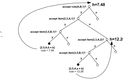
Figure 3: The lookahead heuristic. We set the heuristics for rule and item nodes by looking ahead at the cost of the greedy solution from that point in the search space.

Figure 2 shows two complete search paths for our example, terminated by goal nodes (in black). Notice that the internal nodes of the search space can be classified by the type of decision they govern. To distinguish between these nodes, we will refer to them as subspan nodes, precondition nodes, rule nodes, and item nodes.

We can now proceed to attach heuristics to the nodes and run a heuristic search protocol, say A*, on this search space. For subspan and precondition nodes, we attach trivial uninformative heuristics, i.e. h =−∞. For goal nodes, the heuristic is the actual cost of the item they represent. For rule and item nodes, we will use a simple type of heuristic, often referred to in the literature as a lookahead heuristic. Since the rule nodes and item nodes are ordered, respectively, by rule and item cost, it is possible to “look ahead” at a greedy solution from any of those nodes. See Figure 3. This greedy so-lution is reached by choosing to accept every de-cision presented until we hit a goal node.

4 Cube Pruning as Heuristic Search

In this section, we will compare cube pruning with our A* search protocol, by tracing through their respective behaviors on the simple example of Fig-ure 1.

4.1 Phase 1: Initialization

To fill span [α, β], cube pruning (CP) begins by constructing a cube for each tuple of the form:

h[α, δ],[δ, β], X, Yi

where X and Y are nonterminals. A cube consists of three axes: rules(X,Y)anditems(α, δ,X)and items(δ, β,Y). Figure 4(left) shows the nontrivial cubes for our example scenario.

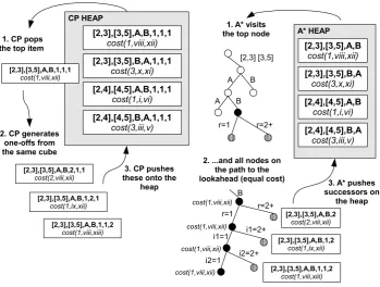
Contrast this with A*, which begins by adding the root node of our search space to an empty heap (ordered by heuristic cost). It proceeds to repeat-edly pop the lowest-cost node from the heap, then add its children to the heap (we refer to this op-eration as visiting the node). Note that before A* ever visits a rule node, it will have visited every subspan and precondition node (because they all have cost h = −∞). Figure 4(right) shows the state of A* at this point in the search. We assume that we do not generate dead-end nodes (a simple matter of checking that there exist applicable rules and items for the chosen subspans and precondi-tions). Observe the correspondence between the cubes and the heap contents at this point in the A* search.

4.2 Phase 2: Seeding the Heap

Cube pruning proceeds by computing the “best” item of each cubeh[α, δ],[δ, β], X, Yi, i.e.

item(α, δ,X,1)⋗rule(X,Y,1)⋖item(δ, β,Y,1)

Because of the interaction cost, there is no guaran-tee that this will really be the best item of the cube, however it is likely to be a good item because the costs of the individual components are low. These items are added to a heap (to avoid confusion, we will henceforth refer to the two heaps as the CP heap and the A* heap), and prioritized by their costs.

Consider again the example. CP seeds its heap with the “best” items of the 4 cubes. There is now a direct correspondence between the CP heap and the A* heap. Moreover, the costs associated with the heap elements also correspond. See Figure 5.

4.3 Phase 3: Finding the First Item

Cube pruning now pops the lowest-cost item from the CP heap. This means that CP has decided to keep the item. After doing so, it forms the “one-off” items and pushes those onto the CP heap. See Figure 5(left). The popped item is:

item (viii)⋗rule (1)⋖item (xii)

CP then pushes the following one-off successors onto the CP heap:

item (viii)⋗rule (2)⋖item (xii)

item (ix)⋗rule (1)⋖item (xii)

item (viii)⋗rule (1)⋖item (xiii)

Contrast this with A*, which pops the lowest-cost search node from the A* heap. Here we need to assume that our A* protocol differs slightly from standard A*. Specifically, it will practice node-tying, meaning that when it visits a rule node or an item node, then it also (atomically) visits all nodes on the path to its lookahead goal node. See Figure 5(right). Observe that all of these nodes have the same heuristic cost, thus standard A* is likely to visit these nodes in succession without the need to enforce node-tying, but it would not be guaranteed (because the heuristics are not ad-missible). A* keeps the goal node it finds and adds the successors to the heap, scored with their looka-head heuristics. Again, note the direct correspon-dence between what CP and A* keep, and what they add to their respective heaps.

4.4 Phase 4: Finding Subsequent Items

Cube pruning and A* continue to repeat Phase 3 until k unique items have been kept. While we could continue to trace through the example, by now it should be clear: cube pruning and our A* protocol with node-tying are doing the same thing at each step. In fact, they are exactly the same algorithm. We do not present a formal proof here; this statement should be regarded as confi-dent conjecture.

Figure 4: (left) Cube formation for our example. (right) The A* protocol, after all subspan and precon-dition nodes have been visited. Notice the correspondence between the cubes and the A* heap contents.

5 Augmented Cube Pruning

Viewed in this light, the idiosyncracies of cube pruning begin to reveal themselves. On the one hand, rule and item nodes are associated with strong but inadmissible heuristics (the short expla-nation for why cube pruning is an inexact algo-rithm). On the other hand, subspan and precondi-tion nodes are associated with weak trivial heuris-tics. This should be regarded neither as a surprise nor a criticism, considering cube pruning’s origins in hierarchical phrase-based MT models (Chiang, 2007), which have only a small number of distinct nonterminals.

But the situation is much different in tree-to-string transducer-based MT (Galley et al., 2004; Galley et al., 2006; DeNero et al., 2009). Transducer-based MT relies on SCFGs with large nonterminal sets. Binarizing the grammars (Zhang et al., 2006) further increases the size of these sets, due to the introduction of virtual nonterminals.

A key benefit of the heuristic search viewpoint is that it is well positioned to take advantage of such insights into the structure of a particular de-coding problem. In the case of transducer-based MT, the large set of preconditions encourages us to introduce a nontrivial heuristic for the precon-dition nodes. The inclusion of these heuristics into the CP search will enable A* to eliminate cer-tain preconditions from consideration, giving us a speedup. For this reason we call this strategy aug-mented cube pruning.

5.1 Heuristics on preconditions

Recall that the total cost of a goal node is given by Equation (6), which has four terms. We will form the heuristic for a precondition node by creating a separate heuristic for each of the four terms and using the sum as the overall heuristic.

To describe these heuristics, we will make intu-itive use of the wildcard operator∗ to extend our existing notation. For instance,items(α, β,*)will denote the union ofitems(α, β,X)over all possi-ble X, sorted by cost.

We associate the heuristic h(δ,X,Y) with the search node reached by choosing subspans[α, δ], [δ, β], precondition X (for span[α, δ]), and precon-dition Y (for span[δ, β]). The heuristic is the sum of four terms, mirroring Equation (6):

h(δ,X,Y) = cost(rule(X,Y,1)) + cost(item(α, δ,X,1)) + cost(item(δ, β,Y,1)) + ih(δ,X,Y)

The first three terms are admissible because each is simply the minimum possible cost of some choice remaining to be made. To con-struct the interaction heuristic ih(δ,X,Y), con-sider that in a translation model with an inte-grated n-gram language model, the interaction costinteraction(r, κ₁, κ₂)is computed by adding the language model costs of any new complete n-grams that are created by combining the carries (boundary words) with each other and with the lexical items on the rule’s target side, taking into account any reordering that the rule may perform. We construct a backoff-style estimate of these new n-grams by looking at item(α, δ,X,1) = [α, δ,X, κ1], item(δ, β,Y,1) = [δ, β,Y, κ₂], and rule(X,Y,1). We set ih(δ,X,Y) to be a linear combination of the backoffn-grams of the carries κ1 andκ₂, as well as anyn-grams introduced by the rule. For instance, if

κ1 = a b ⋄ c d κ2 = e f ⋄ g h

rule(X,Y,1) = Z→ hX0 Y1, X0 g h i Y1i

then

ih(δ,X,Y) = γ₁·LM(a) +γ₂·LM(a b) + γ1·LM(e) +γ₂·LM(e f) + γ1·LM(g) +γ₂·LM(g h) + γ3·LM(g h i)

The coefficients of the combination are free pa-rameters that we can tune to trade off between more pruning and more admissability. Setting the coefficients to zero gives perfect admissibility but is also weak.

The heuristic for the first precondition node is computed similarly:

Standard CP Augmented CP nodes (k) BLEU time nodes (k) BLEU time

80 34.9 2.5 52 34.7 1.9

148 36.1 3.9 92 35.9 2.4

345 37.2 7.9 200 37.3 5.4

520 37.7 13.4 302 37.7 8.5

725 38.2 17.1 407 38.0 10.7

1092 38.3 27.1 619 38.2 16.3 1812 38.6 45.9 1064 38.5 27.7

Table 1: Results of standard and augmented cube pruning. The number of (thousands of) search nodes visited is given along with BLEU and av-erage time to decode one sentence, in seconds.

0 5 0 0 0 0 0 1 x 1 0 6

1 . 5

x 1

0 6 2 x 1

0 6 Searchnodesvisited

3 5 3 6 3 7 3 8

BL

EU

St a n d a r dCP Au g m en tedCP

Figure 6: Nodes visited by standard and aug-mented cube pruning.

We also apply analogous heuristics to the subspan nodes.

5.2 Experimental setup

We evaluated all of the algorithms in this paper on a syntax-based Arabic-English translation system based on (Galley et al., 2006), with rules extracted from 200 million words of parallel data from NIST 2008 and GALE data collections, and with a 4-gram language model trained on 1 billion words of monolingual English data from the LDC Giga-word corpus. We evaluated the system’s perfor-mance on the NIST 2008 test corpus, which con-sists of 1357 Arabic sentences from a mixture of newswire and web domains, with four English ref-erence translations. We report BLEU scores (Pa-pineni et al., 2002) on untokenized, recapitalized output.

5.3 Results for Augmented Cube Pruning

The results for augmented cube pruning are com-pared against cube pruning in Table 1. The data

0 1 0 2 0 3 0 4 0 5 0 A

veragetimepersentence(s) 3 5

3 6 3 7 3 8

BL

EU

St a n d a r dCP Au g m en tedCP

Figure 7: Time spent by standard and augmented cube pruning, average seconds per sentence.

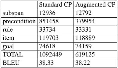
Standard CP Augmented CP

subspan 12936 12792

precondition 851458 379954

rule 33734 33331

item 119703 118889

goal 74618 74159

TOTAL 1092449 619125

BLEU 38.33 38.22

Table 2: Breakdown of visited search nodes by type (for a fixed beam size).

from that table are also plotted in Figure 6 and Figure 7. Each line gives the number of nodes visited by the heuristic search, the average time to decode one sentence, and the BLEU of the out-put. The number of items kept by each span (the beam) is increased in each subsequent line of the table to indicate how the two algorithms differ at various beam sizes. This also gives a more com-plete picture of the speed/BLEU tradeoff offered by each algorithm. Because the two algorithms make the same sorts of lookahead computations with the same implementation, they can be most directly compared by examining the number of visited nodes. Augmenting cube pruning with ad-missible heuristics on the precondition nodes leads to a substantial decrease in visited nodes, by 35-44%. The reduction in nodes converges to a con-sistent 40% as the beam increases. The BLEU with augmented cube pruning drops by an average of 0.1 compared to standard cube pruning. This is due to the additional inadmissibility of the interac-tion heuristic.

size. The precondition heuristic enables A* to prune more than half the precondition nodes.

6 Exact Cube Pruning

Common wisdom is that the speed of cube prun-ing more than compensates for its inexactness (re-call that this inexactness is due to the fact that it uses A* search with inadmissible heuristics). Es-pecially when we move into transducer-based MT, the search space becomes so large that brute-force item generation is much too slow to be practi-cal. Still, within the heuristic search framework we may ask the question: is it possible to apply strictly admissible heuristics to the cube pruning search space, and in so doing, create a version of cube pruning that is both fast and exact, one that finds the n best items for each span and not just ngood items? One might not expect such a tech-nique to outperform cube pruning in practice, but for a given use case, it would give us a relatively fast way of assessing the BLEU drop incurred by the inexactness of cube pruning.

Recall again that the total cost of a goal node is given by Equation (6), which has four terms. It is easy enough to devise strong lower bounds for the first three of these terms by extending the rea-soning of Section 5. Table 3 shows these heuris-tics. The major challenge is to devise an effective lower bound on the fourth term of the cost func-tion, the interaction heuristic, which in our case is the incremental language model cost.

We take advantage of the following observa-tions:

1. In a given span, many boundary word pat-terns are repeated. In other words, for a par-ticular span[α, β]and carry κ, we often see many items of the form [α, β,X, κ], where the only difference is the postcondition X.

2. Most rules do not introduce lexical items. In other words, most of the grammar rules have the form Z → hX₀Y₁, X₀Y₁i (concatena-tion rules) or Z → hX₀ Y₁, Y₁X₀i (inver-sion rules).

The idea is simple. We split the search into three searches: one for concatenation rules, one for in-version rules, and one for lexical rules. Each search finds then–best items that can be created using its respective set of rules. We then take these 3nitems and keep the bestn.

1 0 2 0 3 0 4 0 5 0 6 0 7 0 A

veragetimepersentence(s) 3 5

3 6 3 7 3 8

BL

EU

St a n d a r dCP Exa ctCP

Figure 8: Time spent by standard and exact cube pruning, average seconds per sentence.

Doing this split enables us to precompute a strong and admissible heuristic on the interaction cost. Namely, for a given span [α, β], we pre-compute ih_adm(δ,X,Y), which is the best LM cost of combining carries from items(α, δ,X) and items(δ, β,Y). Notice that this statistic is only straightforward to compute once we can as-sume that the rules are concatenation rules or inversion rules. For the lexical rules, we set ihadm(δ,X,Y) = 0, an admissible but weak heuristic that we can fortunately get away with be-cause of the small number of lexical rules.

6.1 Results for Exact Cube Pruning

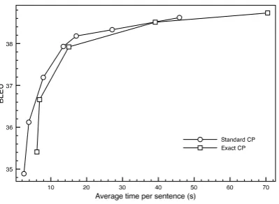
Computing the ih_adm(δ,X,Y) heuristic is not cheap. To be fair, we first compare exact CP to standard CP in terms of overall running time, in-cluding the computational cost of this overhead. We plot this comparison in Figure 8. Surprisingly, the time/quality tradeoff of exact CP is extremely similar to standard CP, suggesting that exact cube pruning is actually a practical alternative to stan-dard CP, and not just of theoretical value. We found that the BLEU loss of standard cube prun-ing at moderate beam sizes was between 0.4 and 0.6.

heuristic components

subspan precondition1 precondition2 rule item1 item2

h(δ) h(δ,X) h(δ,X,Y) h(δ,X,Y, i) h(δ,X,Y, i, j) h(δ,X,Y, i, j, k) r rule(∗,∗,1) rule(X,∗,1) rule(X,Y,1) rule(X,Y, i) rule(X,Y, i) rule(X,Y, i) ι1 item(α, δ,∗,1) item(α, δ,X,1) item(α, δ,X,1) item(α, δ,X,1) item(α, δ,X, j) item(α, δ,X, j)

ι2 item(δ, β,∗,1) item(δ, β,∗,1) item(δ, β,Y,1) item(δ, β,Y,1) item(δ, β,Y,1) item(δ, β,Y, k)

ih ihadm(δ,∗,∗) ihadm(δ,X,∗) ihadm(δ,X,Y) ih_adm(δ,X,Y) ih_adm(δ,X,Y) ih_adm(δ,X,Y)

Table 3: Admissible heuristics for exact CP. We attach heuristic h(δ,X,Y, i, j, k) to the search node reached by choosing subspans [α, δ],[δ, β], preconditions X and Y, the ith rule of rules(X,Y), thejth item ofitem(α, δ,X), and the kth item ofitem(δ, β,Y). To form the heuristic for a particular type of search node (column), compute the following: cost(r) +cost(ι₁) +cost(ι₂) +ih

5 0 0 0 0 0 1 x 1 0 6

1 . 5

x 1

0 6 2 x 1

0 6 Searchnodesvisited

3 5 3 6 3 7 3 8

BL

EU

St a n d a r dCP Exa ctCP

Figure 9: Nodes visited by standard and exact cube pruning.

7 Implications

This paper’s core idea is the utility of framing CKY item generation as a heuristic search prob-lem. Once we recognize cube pruning as noth-ing more than A* on a particular search space with particular heuristics, this deeper understand-ing makes it easy to create faster and exact vari-ants for other use cases (in this paper, we focus on tree-to-string transducer-based MT). Depend-ing on one’s own particular use case, a variety of possibilities may present themselves:

1. What if we try different heuristics? In this pa-per, we do some preliminary inquiry into this question, but it should be clear that our minor changes are just the tip of the iceberg. One can easily imagine clever and creative heuris-tics that outperform the simple ones we have proposed here.

2. What if we try a different search space? Why are we using this particular search space? Perhaps a different one, one that makes

de-cisions in a different order, would be more effective.

3. What if we try a different search algorithm? A* has nice guarantees (Dechter and Pearl, 1985), but it is space-consumptive and it is not anytime. For a use case where we would like a finer-grained speed/quality tradeoff, it might be useful to consider an anytime search algorithm, like depth-first branch-and-bound (Zhang and Korf, 1995).

By working towards a deeper and unifying under-standing of the smorgasbord of current MT speed-up techniques, our hope is to facilitate the task of implementing such methods, combining them ef-fectively, and adapting them to new use cases.

Acknowledgments

We would like to thank Abdessamad Echihabi, Kevin Knight, Daniel Marcu, Dragos Munteanu, Ion Muslea, Radu Soricut, Wei Wang, and the anonymous reviewers for helpful comments and advice. Thanks also to David Chiang for the use of his LaTeX macros. This work was supported in part by CCS grant 2008-1245117-000.

References

David Chiang. 2007. Hierarchical phrase-based trans-lation. Computational Linguistics, 33(2):201–228.

Rina Dechter and Judea Pearl. 1985. Generalized best-first search strategies and the optimality of a*.

Jour-nal of the ACM, 32(3):505–536.

John DeNero, Mohit Bansal, Adam Pauls, and Dan Klein. 2009. Efficient parsing for transducer gram-mars. In Proceedings of the Human Language

Michel Galley, Mark Hopkins, Kevin Knight, and Daniel Marcu. 2004. What’s in a translation rule? In Proceedings of HLT/NAACL.

Michel Galley, Jonathan Graehl, Kevin Knight, Daniel Marcu, Steve DeNeefe, Wei Wang, and Ignacio Thayer. 2006. Scalable inference and training of context-rich syntactic models. In Proceedings of

ACL-COLING.

Liang Huang and David Chiang. 2007. Forest rescor-ing: Faster decoding with integrated language mod-els. In Proceedings of ACL.

Robert C. Moore and Chris Quirk. 2007. Faster beam-search decoding for phrasal statistical ma-chine translation. In Proceedings of MT Summit XI.

Kishore Papineni, Salim Roukos, Todd Ward, and Wei-Jing Zhu. 2002. Bleu: a method for automatic evaluation of machine translation. In Proceedings

of 40th Annual Meeting of the Association for Com-putational Linguistics, pages 311–318.

Judea Pearl. 1984. Heuristics. Addison-Wesley.

Slav Petrov, Aria Haghighi, and Dan Klein. 2008. Coarse-to-fine syntactic machine translation using language projections. In Proceedings of EMNLP.

Michael Pust and Kevin Knight. 2009. Faster mt de-coding through pervasive laziness. In Proceedings

of NAACL.

Brian Roark and Kristy Hollingshead. 2008. Classi-fying chart cells for quadratic complexity context-free inference. In Proceedings of the 22nd

Inter-national Conference on Computational Linguistics (Coling 2008), pages 745–752.

Brian Roark and Kristy Hollingshead. 2009. Lin-ear complexity context-free parsing pipelines via chart constraints. In Proceedings of Human

Lan-guage Technologies: The 2009 Annual Conference of the North American Chapter of the Associa-tion for ComputaAssocia-tional Linguistics, pages 647–655,

Boulder, Colorado, June. Association for Computa-tional Linguistics.

Weixiong Zhang and Richard E. Korf. 1995. Perfor-mance of linear-space search algorithms. Artificial

Intelligence, 79(2):241–292.

Hao Zhang, Liang Huang, Daniel Gildea, and Kevin Knight. 2006. Synchronous binarization for ma-chine translation. In Proceedings of the Human