The Economic and Social Review, Vol. 27, No. 4, July, 1996, pp. 341-363
Mapping Disease R i s k Estimates Based on
Small Numbers: A n Assessment of E m p i r i c a l
Bayes Techniques*
D.G. P R I N G L E
St. Patrick's College, Maynooth
Abstract: Choropleth maps are frequently used to analyse spatial variations in the r i s k of a
disease. I n such maps the relative risk is typically quantified by dividing some measure of the number of cases of the disease by some measure of the population at risk. T h e resulting rates may be regarded as m a x i m u m likelihood estimates of individual risk. These estimates may be unstable i f the areas are very small or if the disease is rare. I n such situations, the highest and lowest v a l u e s on the m a p w i l l display a tendency to be concentrated in the a r e a s w i t h the smallest populations. T h e traditional solution to this problem is to supplement m a p s based on ratios w i t h probability maps. However, probability maps display an opposite bias — i.e., they tend to highlight the areas with the largest populations. Several statisticians have suggested a compromise between these two extremes using empirical B a y e s techniques. T h i s paper outlines the rationale underlying empirical Bayes techniques, and assesses their usefulness using case studies of neo-natal mortality and cancer mortality.
I I N T R O D U C T I O N
M
aps o f t h e prevalence or incidence o f a disease often provide useful aetiological i n f o r m a t i o n about t h e possible causes o f t h a t disease. A heightened incidence o f a p a r t i c u l a r disease i n c e r t a i n areas could reflect t h e effects o f either "contextual" factors such as local e n v i r o n m e n t a l r i s k s (e.g., a p o l l u t i o n or r a d i a t i o n source), or "compositional" factors such as a h i g h e r per centage o f people w h o as i n d i v i d u a l s have a h i g h e r r i s k because o f geneticfactors or h i g h r i s k behaviours (Duncan et al., 1993). Conversely, the absence of a h e i g h t e n e d incidence m a y help to a l l e v i a t e u n j u s t i f i e d public concern about a non-dangerous facility. Disease maps can also a i d decision m a k i n g by h e a l t h service policy m a k e r s , w h e t h e r t h e i r p r i m a r y concern is disease p r e v e n t i o n or t h e p r o v i s i o n of services for medical t r e a t m e n t . Some h e a l t h r i s k factors, such as p o l l u t i o n sources or h i g h r i s k behaviours (e.g., smoking), m a y be amenable t o p r e v e n t i v e strategies; other r i s k factors (such as age, race or gender) obviously are n o t , b u t a knowledge o f t h e spatial d i s t r i b u t i o n of these factors m a y facilitate t h e provision of a more efficient h e a l t h delivery system.
Disease m a p p i n g is by no means unproblematic. There are a large n u m b e r of s t a t i s t i c a l problems w h i c h have to be addressed — some of w h i c h are by no means obvious. There are also a large n u m b e r of cartographic p i t f a l l s a w a i t i n g t h e inexperienced map-maker. Maps can create a powerful v i s u a l image, b u t t h e y can also create a v e r y m i s l e a d i n g i m p r e s s i o n either by accident or design ( M o n m o n i e r , 1991). T h e meaningful i n t e r p r e t a t i o n of disease maps is therefore contingent u p o n an awareness of t h e potential problems.
T h e r e are a t present c o m p a r a t i v e l y few examples of disease m a p p i n g i n I r e l a n d , a l t h o u g h i t is envisaged t h a t t h i s s i t u a t i o n w i l l change r a p i d l y w i t h i n c r e a s e d a d o p t i o n o f geographical i n f o r m a t i o n systems (GIS). Dawson's (1911) s t u d y o f " i n s a n i t y " provides a n i n t e r e s t i n g early example o f a disease m a p ( e s p e c i a l l y w h e n c o m p a r e d w i t h m a p s o f r e p o r t e d s c h i z o p h r e n i a m o r b i d i t y a t present), b u t m o s t o f t h e more recent examples o f disease m a p p i n g t e n d t o be based o n m o r t a l i t y d a t a . The C e n t r a l Statistics Office n o r m a l l y includes maps of m o r t a l i t y i n the Report on Vital Statistics w h i c h i t compiles each year for t h e D e p a r t m e n t o f H e a l t h . However, these maps are based on d a t a w h i c h are standardised for v a r i a t i o n s i n p o p u l a t i o n s t r u c t u r e u s i n g t h e d i r e c t method. T h i s tends to a m p l i f y m i n o r stochastic fluctuations, t h e r e b y d i s g u i s i n g a e t i o l o g i c a l l y i m p o r t a n t r e g u l a r i t i e s i n t h e u n d e r l y i n g v a r i a t i o n s i n r i s k . I n d i r e c t s t a n d a r d i s a t i o n , as used for example by H o w e l l et al. (1993), is preferable, a l t h o u g h the s p a t i a l v a r i a t i o n s displayed i n such maps t e n d t o be d o m i n a t e d by v a r i a t i o n s i n t h e number of deaths i n t h e older age cohorts. P r i n g l e (1986) a t t e m p t e d to overcome t h i s p a r t i c u l a r p r o b l e m , w i t h m i x e d success, by calculating a n " U n f u l f i l l e d Life Index".
(1983; 1987) i n studies of Belfast a n d D u b l i n aggregated a d j o i n i n g areas. B o t h strategies provide only p a r t i a l solutions.
The " s m a l l n u m b e r s " problem is probably the m o s t pervasive p r o b l e m i n disease m a p p i n g . T h e problem arises w h e n t h e absolute n u m b e r of cases o f the disease i n each area is s m a l l , e i t h e r because the areas are v e r y s m a l l or the disease is c o m p a r a t i v e l y r a r e or b o t h . W h e n used as t h e n u m e r a t o r s t o calculate rates, s m a l l n u m b e r s m a y provide v e r y m i s l e a d i n g impressions o f t h e u n d e r l y i n g r i s k s . S i m i l a r problems are associated w i t h other social a n d economic i n d i c a t o r s expressed as rates or r a t i o s for s m a l l areas (e.g., u n e m p l o y m e n t rates, per capita income). Possible solutions, based o n e m p i r i c a l Bayes techniques, have been proposed by v a r i o u s s t a t i s t i c i a n s i n r e c e n t years. These techniques form the focus of the present paper. The paper begins by e x p l a i n i n g the s m a l l n u m b e r s p r o b l e m i n more d e t a i l a n d t h e n o u t l i n e s some o f t h e strategies w h i c h have t r a d i t i o n a l l y been adopted to t r y to c i r c u m v e n t t h e p r o b l e m . A l t e r n a t i v e approaches based o n e m p i r i c a l Bayes tech niques are t h e n i n t r o d u c e d . The f i n a l p a r t of t h e paper reports a n e m p i r i c a l assessment o f the effectiveness of these techniques u s i n g case studies o f neo n a t a l m o r t a l i t y and deaths from cancer.
I I T H E S M A L L N U M B E R S P R O B L E M
N o r m a l l y w h e n one maps t h e incidence or prevalence o f a disease one is p r i m a r i l y interested i n the s p a t i a l d i s t r i b u t i o n of i n d i v i d u a l r i s k s — i.e., t h e question we w i s h to address is: do people l i v i n g i n some areas have a h i g h e r r i s k o f disease t h a n people i n o t h e r areas? Age specific r a t e s p r o v i d e m a x i m u m l i k e l i h o o d estimates of t h e i n d i v i d u a l r i s k i n a g i v e n age cohort — i.e., t h e m a x i m u m l i k e l i h o o d estimate o f t h e i n d i v i d u a l r i s k 6jj for people i n age group j i n area i is given b y d i v i d i n g the n u m b e r o f cases o f the disease dy amongst people i n age group j i n area i by t h e corresponding p o p u l a t i o n a t r i s k Py.
e
s= d
y/ p
s( i )
Age s t a n d a r d i s e d r a t e s a n d r a t i o s (e.g., standardised m o r t a l i t y r a t i o s ) are essentially w e i g h t e d sums o f age specific rates a n d are consequently subject to s i m i l a r problems. However, i n t h e interests of c l a r i t y , discussion w i l l be confined here t o age specific rates for a single age group.
incidence or prevalence of t h e disease is s m a l l (i.e., i f i t is a rare disease). I f t h e n u m e r a t o r s are s m a l l , t h e r e s u l t i n g estimates o f r i s k w i l l become v e r y u n s t a b l e — i.e., one case m o r e or one case less w i l l m a k e a large percentage difference. F o r example, consider a disease w i t h a n average incidence o f one case i n 1,000, i n t w o areas A a n d B h a v i n g populations of
10,000 a n d 1,000 respectively. The expected n u m b e r of cases i n area A w o u l d be 10 (i.e., 10,000/1,000). I f t h e r e were a c t u a l l y 11 cases, t h e estimated r i s k for t h a t area w o u l d increase to 1.1 per 1,000, whereas i f t h e n u m b e r of cases was one below t h e expected value t h e r a t e w o u l d be 0.9 per 1,000 — either way, t h e r e w o u l d be c o m p a r a t i v e l y l i t t l e change. H o w e v e r , t h e expected n u m b e r o f cases i n area B is only 1 (i.e., 1,000/1,000). I f t h e r e was one case less t h a n expected i n a g i v e n year, t h e r a t e for t h a t area w o u l d f a l l to 0.0; w h i l s t i f t h e r e was one case more t h a n expected, t h e r a t e w o u l d increase to 2.0. I n o t h e r w o r d s , t h e r a t e s for t h e s m a l l e r area could f l u c t u a t e f r o m e x t r e m e l y l o w t o e x t r e m e l y h i g h , possibly r e f l e c t i n g n o t h i n g m o r e t h a n stochastic v a r i a t i o n s . The n e t effect of t h i s is t h a t t h e extreme values o n a choropleth m a p of estimated r i s k s (whether extremely l o w or extremely h i g h ) w i l l d i s p l a y a tendency to be concentrated i n the s m a l l e r areas. G i v e n t h a t t h e extreme values are the ones w h i c h a t t r a c t most a t t e n t i o n w h e n i n t e r p r e t i n g t h e m a p , t h e r e is a n obvious danger o f c r e a t i n g a very m i s l e a d i n g impres sion of t h e s p a t i a l d i s t r i b u t i o n of disease r i s k .
Table 1: The Small Numbers Problem
Area A AreaB
Population A t Risk 10,000 1,000
Expected Cases 10 1
Rate I f + 1 Case 1.1 2.0
Rate I f - 1 Case 0.9 0.0
different diseases w i t h different causal processes being m i x e d a n d confused. A f u r t h e r response to t h e s m a l l n u m b e r s problem (often i n a d d i t i o n t o one or more of t h e strategies o u t l i n e d above) is to supplement the c h o r o p l e t h m a p of e s t i m a t e d r i s k s w i t h a p r o b a b i l i t y m a p i n d i c a t i n g w h i c h areas have a significantly h i g h or a significantly l o w n u m b e r o f cases. These p r o b a b i l i t i e s are u s u a l l y calculated based on t h e assumption t h a t the u n d e r l y i n g r i s k s are t h e same i n a l l areas and t h a t the n u m b e r of cases i n each area is t h e product of a Poisson process. I f t h e c u m u l a t i v e p r o b a b i l i t y calculated u n d e r these assumptions is v e r y large or very s m a l l , t h e n the observed n u m b e r o f cases m a y be designated "significantly h i g h " or " s i g n i f i c a n t l y l o w " ( C h o y n o w s k i , 1959; Giggs et al., 1980; W h i t e , 1972). However, t h i s "solution" also r u n s i n t o problems i f t h e numbers are small. I t is q u i t e possible for there t o be no cases at a l l i n a n area, y e t i f t h e area has a s m a l l p o p u l a t i o n a t r i s k even zero cases m a y n o t be l o w enough to be r e g a r d e d as "significant". L i k e w i s e , a m u c h h i g h e r prevalence is r e q u i r e d i n a s m a l l area for the n u m b e r of cases t o be regarded as significantly h i g h . The n e t effect of t h i s is t h a t p r o b a b i l i t y maps t e n d to create a n impression w h i c h is biased i n favour o f t h e l a r g e r (i.e., more populous) areas (Kaldor a n d C l a y t o n , 1989). U r b a n areas are therefore more l i k e l y t o be i d e n t i f i e d as h a v i n g a s i g n i f i c a n t l y h i g h or a s i g n i f i c a n t l y l o w n u m b e r of cases t h a n less populous r u r a l areas.
T h u s , t o summarise, choropleth maps of the e s t i m a t e d r i s k t e n d t o focus a t t e n t i o n o n t h e s m a l l e r areas, whereas p r o b a b i l i t y m a p s t e n d t o focus a t t e n t i o n on t h e l a r g e r areas. C l e a r l y w e need some s o r t o f c o m p r o m i s e b e t w e e n these t w o extremes. Several b i o s t a t i s t i c i a n s have suggested t h a t e m p i r i c a l Bayes techniques offer a possible solution.
I l l T H E E M P I R I C A L B A Y E S A P P R O A C H
The observed n u m b e r of cases of the disease dy i n age group j i n area i m a y be regarded as t h e outcome o f a Poisson process w i t h a n e x p e c t a t i o n OyPjj w h e r e 0y is the u n d e r l y i n g r i s k a n d p4j is t h e n u m b e r o f people a t r i s k . H o w ever, t h e observed n u m b e r o f cases m a y be e i t h e r h i g h e r or l o w e r t h a n the expected n u m b e r , due t o stochastic v a r i a t i o n s . T h e basic objective is t o estimate a n d m a p t h e u n k n o w n u n d e r l y i n g r i s k 9;j for each area u s i n g t h e i n f o r m a t i o n available o n t h e observed numbers of cases. The p r o b l e m is t h a t , for any given area, one does not k n o w w h e t h e r t h e observed n u m b e r o f cases is h i g h e r or l o w e r t h a n t h e expected n u m b e r ( w h i c h is g o v e r n e d b y t h e u n k n o w n u n d e r l y i n g r i s k ) or by how m u c h .
section) i t m a y be subject to v e r y large stochastic fluctuations as a r e s u l t of t h e s m a l l n u m b e r s p r o b l e m . T h e basic premise of t h e e m p i r i c a l Bayes approach is t h a t w e do i n fact have access to a d d i t i o n a l i n f o r m a t i o n w h i c h m a y be i n c o r p o r a t e d i n t h e e s t i m a t i o n process to produce more realistic esti mates of t h e u n d e r l y i n g risks.
To u n d e r s t a n d t h e n a t u r e of t h i s a d d i t i o n a l i n f o r m a t i o n , i t is i n s t r u c t i v e to consider a n e x t r e m e h y p o t h e t i c a l s i t u a t i o n i n w h i c h we have perfect infor m a t i o n for every area except one — for w h i c h we have no i n f o r m a t i o n whatso ever ( K a l d o r a n d C l a y t o n , 1989). A p p l y i n g t h e m a x i m u m l i k e l i h o o d f o r m u l a we w o u l d be u n a b l e t o say a n y t h i n g at a l l about the r i s k i n t h e area w i t h t h e m i s s i n g d a t a . H o w e v e r , i t does n o t seem unreasonable to assume t h a t t h e r i s k i n t h i s area is probably of t h e same order o f m a g n i t u d e as t h e r i s k s i n t h e areas for w h i c h we do have i n f o r m a t i o n . Indeed, i f the r i s k s i n t h e other areas d i s p l a y a h i g h degree of s p a t i a l order, we m a y even be j u s t i f i e d i n c o n c l u d i n g t h a t t h e r i s k i n t h e area w i t h the m i s s i n g data is s i m i l a r t o t h e r i s k s i n t h e areas w h i c h border u p o n i t . I n other words, we could use our knowledge of t h e d i s t r i b u t i o n o f r i s k s i n general to say something about a n area for w h i c h w e have no e m p i r i c a l i n f o r m a t i o n whatsoever.
A s i m i l a r logic m a y be applied i n more n o r m a l circumstances to areas for w h i c h we do have e m p i r i c a l data. I f t h e m a x i m u m likelihood estimate o f t h e r i s k i n a n a r e a i s e x t r e m e l y h i g h or e x t r e m e l y l o w t h e n i t w o u l d seem reasonable to modify i t i n the l i g h t of w h a t we k n o w about the d i s t r i b u t i o n of r i s k s i n o t h e r areas. The r e s u l t i n g estimate of t h e u n d e r l y i n g r i s k for each a r e a m a y therefore be r e g a r d e d as a compromise between t h e m a x i m u m l i k e l i h o o d e s t i m a t e based u p o n t h e observed n u m b e r of cases a n d t h e overall r i s k for t h e e n t i r e s t u d y area. T h e balance between these t w o components s h o u l d reflect t h e r e l i a b i l i t y of t h e e m p i r i c a l data: i f the area is large, t h e n t h e m a x i m u m l i k e l i h o o d estimate should receive most weight; however, i f t h e area is s m a l l , a n d the m a x i m u m l i k e l i h o o d estimates could be subject to large stochastic fluctuations, t h e n t h e o v e r a l l mean should receive more w e i g h t .
These objectives m a y be achieved w i t h i n a Bayesian framework. Bayesian s t a t i s t i c s are based u p o n t h e observation t h a t t h e j o i n t p r o b a b i l i t y o f t w o events A a n d B is equal to the p r o b a b i l i t y o f the f i r s t times t h e p r o b a b i l i t y o f t h e second c o n d i t i o n a l u p o n the f i r s t (Iverson, 1984):
T h o m a s Bayes, a n e i g h t e e n t h c e n t u r y clergyman, used t h i s r e l a t i o n s h i p to develop a t h e o r e m w h i c h may be w r i t t e n as:
p ( A B ) = p ( A ) . p ( B I A ) (2)
p(6lx) = p(xie).p(0) (3)
where x is the observed d a t a a n d 9 is a n u n k n o w n parameter to be e s t i m a t e d ( i n o u r case, the r i s k of disease). The left h a n d side o f t h e equation is referred t o as t h e posterior d i s t r i b u t i o n , a n d i t describes t h e d i s t r i b u t i o n of possible values for t h e parameter c o n d i t i o n a l u p o n t h e observed data. T h e t e r m p(9) on t h e r i g h t h a n d side, r e f e r r e d to as the prior d i s t r i b u t i o n , describes w h a t we k n o w about t h e d i s t r i b u t i o n of possible parameter values before observing t h e data. The b o t t o m l i n e on t h e r i g h t h a n d side is a n o r m a l i s i n g constant w h i c h integrates to u n i t y , w h i l s t t h e t e r m p(x I 9) m a y be i n t e r p r e t e d as t h e l i k e l i h o o d of 9 given data x. Bayes theorem m a y therefore be s u m m a r i s e d as:
posterior d i s t r i b u t i o n « likelihood function x p r i o r d i s t r i b u t i o n
I n t h e context of disease m a p p i n g , the p r i o r d i s t r i b u t i o n expresses o u r i n i t i a l belief about the d i s t r i b u t i o n o f u n d e r l y i n g r i s k s between areas, the l i k e l i h o o d f u n c t i o n is t h e Poisson d i s t r i b u t e d n u m b e r o f cases c o n d i t i o n a l o n t h e t r u e r i s k i n each area, a n d the posterior d i s t r i b u t i o n is t h e d i s t r i b u t i o n o f possible values for t h e u n d e r l y i n g r i s k i n each area c o n d i t i o n a l u p o n t h e observed n u m b e r of cases.
T h e researcher m u s t m a k e assumptions about t h e n a t u r e o f t h e p r i o r d i s t r i b u t i o n o f t h e u n d e r l y i n g r i s k s a n d t h e l i k e l i h o o d f u n c t i o n . I n a f u l l B a y e s i a n approach t h e researcher w o u l d be r e q u i r e d to specify t h e p r i o r d i s t r i b u t i o n i n i t s e n t i r e t y , b u t i n a n empirical Bayes approach t h e researcher need only m a k e a n assumption about t h e n a t u r e of t h e p r i o r d i s t r i b u t i o n . The p a r a m e t e r s o f t h e p r i o r d i s t r i b u t i o n are t h e n e s t i m a t e d from t h e observed d a t a ( B a i l e y a n d G a t r e l l , 1 9 9 5 ) .1 T h i s p r i o r d i s t r i b u t i o n is t h e n c o m b i n e d w i t h t h e l i k e l i h o o d f u n c t i o n t o give t h e posterior d i s t r i b u t i o n . T h e m e a n of t h e posterior d i s t r i b u t i o n provides a n e m p i r i c a l Bayes estimate o f t h e under l y i n g r i s k .
Applications of the e m p i r i c a l Bayes approach v a r y i n t h e i r choice o f a p r i o r d i s t r i b u t i o n . A G a m m a d i s t r i b u t i o n is often preferred because i t is i n t u i t i v e l y reasonable a n d results i n c o m p a r a t i v e l y simple calculations, due t o t h e fact t h a t a G a m m a d i s t r i b u t i o n combined w i t h a Poisson d i s t r i b u t i o n gives a N e g a t i v e B i n o m i a l d i s t r i b u t i o n (e.g., C l a y t o n a n d K a l d o r , 1987; L a n g f o r d , 1994; M a n t o n et al., 1987; Stone, 1988; T s u t a k a w a , 1988). O t h e r p u b l i s h e d studies assume a N o r m a l d i s t r i b u t i o n o f t h e l o g i t s o f t h e r e l a t i v e r i s k s (e.g., T s u t a k a w a et al., 1985); a N o r m a l d i s t r i b u t i o n o f t h e F r e e m a n - T u k e y
t r a n s f o r m e d r i s k s (Cressie, 1993); a L o g - N o r m a l d i s t r i b u t i o n (e.g., C l a y t o n a n d K a l d o r , 1987); a B e t a d i s t r i b u t i o n (e.g., M i y a w a k i a n d Chen, 1981); a u n i f o r m d i s t r i b u t i o n (e.g., H e i s t e r k a m p , 1993); or even a n o n - p a r a m e t r i c m o d e l (e.g., C l a y t o n a n d K a l d o r , 1987; H e i s t e r k a m p , 1993). The choice of p r i o r d i s t r i b u t i o n clearly influences the m e t h o d of calculation a n d the values of t h e r e s u l t i n g estimates: t h e e m p i r i c a l Bayes approach should therefore be regarded as a f a m i l y of techniques r a t h e r t h a n a single method.
M o s t o f these models are u n f o r t u n a t e l y m a t h e m a t i c a l l y complex. The case studies below use the G a m m a model developed by C l a y t o n a n d K a l d o r (1987). T h i s is p r o b a b l y t h e best k n o w n model a n d has the advantage t h a t i t can be expanded to accommodate s i t u a t i o n s where i t is necessary to take account o f v a r i a t i o n s i n age composition (as i n t h e second case study reported below). C l a y t o n a n d K a l d o r ' s m o d e l assumes t h a t t h e r e l a t i v e r i s k s 6; follow a G a m m a d i s t r i b u t i o n w i t h a scale parameter a, and a shape parameter v (i.e., m e a n v / a a n d variance v / a2) a n d t h a t t h e observed n u m b e r of cases 0 ; are Poisson v a r i a t e s w i t h a n expectation 9 j E; where E; is t h e n u m b e r o f cases w o u l d be expected i n area i g i v e n i t s p o p u l a t i o n at r i s k . C l a y t o n a n d K a l d o r derive t w o e q u a t i o n s w h i c h c a n be used r e c u r s i v e l y t o estimate t h e p a r ameters a and v :
T h e a u t h o r is u n a w a r e o f a n y commercially available software t o solve for a a n d v, so i t i s necessary t o w r i t e one's o w n . T h e procedure requires one t o s u b s t i t u t e estimates of a a n d v i n t o the r i g h t h a n d sides of Equations (4) a n d (5). A n e w e s t i m a t e for a m a y t h e n be obtained by d i v i d i n g t h e answer for E q u a t i o n (4) b y t h e answer for E q u a t i o n (5). T h i s m a y t h e n be s u b s t i t u t e d i n t o E q u a t i o n (4) to get a n e w e s t i m a t e o f v. The w h o l e procedure is t h e n repeated u n t i l t h e e s t i m a t e d values o f a a n d v stabilise between i t e r a t i o n s . H a v i n g solved for a a n d v, t h e posterior expectation o f 0; conditional o n 0 , is given by:
a v
(4)
(5)
E ( eiI Oi; a , v ) = O j + v E i + a
T h i s provides t h e e m p i r i c a l Bayes estimates of t h e r e l a t i v e r i s k s for each area. These m a y be converted i n t o rates by s i m p l y m u l t i p l y i n g t h e m by t h e overall rate.
I V CASE S T U D I E S
M o s t p u b l i s h e d studies of e m p i r i c a l Bayes techniques provide a d e t a i l e d m a t h e m a t i c a l a r g u m e n t i n favour of a p a r t i c u l a r approach, b u t provide l i t t l e concrete evidence to support the contention t h a t e m p i r i c a l Bayes techniques are superior t o more t r a d i t i o n a l m a x i m u m l i k e l i h o o d techniques. T h i s section of t h e paper therefore a t t e m p t s to provide an objective assessment of t h e i r u t i l i t y based u p o n case studies of neo-natal deaths a n d female deaths f r o m cancer i n I r e l a n d i n 1989 a n d 1990 — t h e last t w o years for w h i c h t h e Report on Vital Statistics is available at the t i m e of w r i t i n g . I n b o t h studies t h e d a t a are disaggregated by county and county borough.
Case Study 1 : Neo-Natal Mortality, 1989
Neo-natal m o r t a l i t y (i.e., deaths before 4 weeks) provides a suitable subject for assessment purposes. The neo-natal m o r t a l i t y rate is calculated b y d i v i d i n g t h e t o t a l n u m b e r o f neo-natal deaths i n a g i v e n year by t h e t o t a l n u m b e r of l i v e b i r t h s i n the same y e a r .2 B o t h figures m a y be d i r e c t l y o b t a i n e d f r o m the Report on Vital Statistics, thereby e l i m i n a t i n g the possibility o f a d d i t i o n a l complications associated w i t h other m o r t a l i t y or m o r b i d i t y rates a r i s i n g f r o m t h e need to estimate t h e p o p u l a t i o n a t r i s k for inter-censal years or f r o m t h e need t o t a k e account o f i n t e r - c o u n t y v a r i a t i o n s i n age c o m p o s i t i o n . T h e n u m b e r o f neo-natal deaths is also s m a l l enough t o m a k e estimates o f t h e u n d e r l y i n g r i s k i n most counties extremely problematic, t h e r e b y p r o v i d i n g a difficult challenge to t h e methods u n d e r scrutiny.
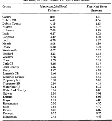
The t o t a l n u m b e r o f live b i r t h s i n 1989 was 52,018; w h i l s t the t o t a l n u m b e r of neo-natal deaths was 249, g i v i n g a n a t i o n a l death r a t e of 4.8 per t h o u s a n d . The absolute n u m b e r s o f deaths per county v a r i e d f r o m a l o w o f 0 (Roscom m o n ) to a h i g h of 37 i n D u b l i n County. The n u m b e r of b i r t h s v a r i e d f r o m a low o f 355 ( L e i t r i m ) t o a h i g h o f 8,825 i n D u b l i n County. The r e s u l t i n g r a t e s per county ranged from a l o w o f 0.0 (Roscommon) to a h i g h o f 9.46 ( L i m e r i c k CB).
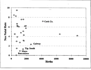
I f we g r a p h t h e calculated neo-natal m o r t a l i t y rates against t h e n u m b e r o f b i r t h s ( F i g u r e 1), we can see t h a t t h e neo-natal rates i n counties w i t h less
t h a n 2,000 b i r t h s (i.e., t h e m a j o r i t y of counties) v a r y from very low to very h i g h . T h e r a t e s for t h e l a r g e r areas (i.e., areas w i t h most b i r t h s ) t e n d to be more i n l i n e w i t h the n a t i o n a l average. T h i s m a y be because the u n d e r l y i n g r i s k s for t h e l a r g e r areas j u s t happen t o f a l l i n the m i d d l e range, b u t a more l i k e l y e x p l a n a t i o n is t h a t the observed v a r i a t i o n s i n t h e smaller counties are a f u n c t i o n of t h e s m a l l n u m b e r s p r o b l e m (i.e., one e x t r a death i n a s m a l l county could move i t from t h e "low r i s k " category i n t o a " h i g h r i s k " category).
10
8
-«
« 63
es Z
O 4 u
Z
2
--o --o
. 1 ® . . .CP.
®
<s>
© Cork Co.
®
© Galway
> @ Tip. South
® Mayo Roscununun
•+-2000 4000 6000
Births
[image:10.479.53.417.182.460.2]8000 10000
Figure 1: Maximum Likelihood Estimates ofNeo-Natal Mortality Rates in 1989 Graphed Against the Number of Births.
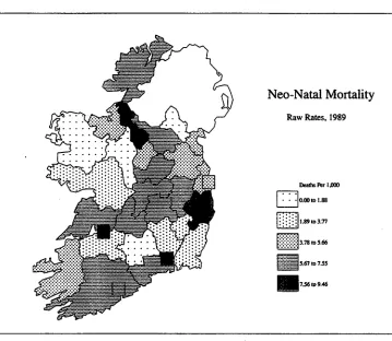
A s a r e s u l t , t h e spatial d i s t r i b u t i o n of m o r t a l i t y rates (Figure 2) cannot be regarded as a reliable i n d i c a t o r o f t h e spatial d i s t r i b u t i o n of risks, given t h e s m a l l n u m b e r s o f deaths i n most of t h e counties. The n o r m a l procedure w o u l d be t o t e s t t h e rates i n each area for s t a t i s t i c a l significance. D o i n g t h i s , i t is f o u n d t h a t C o r k C o u n t y has a s i g n i f i c a n t l y h i g h n u m b e r of deaths, a n d four counties ( T i p p e r a r y South, G a l w a y , M a y o a n d Roscommon) have a s i g n i f i c a n t l y l o w n u m b e r o f deaths.
Figure 2: Spatial Distribution of Maximum Likelihood Estimates of Neo-Natal Mortality Rates in 1989.
h i g h n u m b e r of deaths, i t h a d only t h e s i x t h highest rate. T h i s indicates t h a t t h e rates for t h e 5 counties h a v i n g a h i g h e r r a t e probably need to be i n t e r preted w i t h caution due to the fact t h a t t h e y are not significant. However, i t m a y also reflect t h e tendency for significance tests to favour t h e more popu lous areas (such as C o r k County). T h e significance tests i d e n t i f y t h e t h r e e areas w i t h t h e lowest rates as h a v i n g a s i g n i f i c a n t l y l o w n u m b e r o f deaths, b u t t h e area w i t h t h e f o u r t h lowest r a t e ( M o n a g h a n ) is n o t s i g n i f i c a n t , whereas G a l w a y w i t h a higher death r a t e is significant. A g a i n t h e r e m a y be a tendency for t h e t e s t t o favour t h e l a r g e r areas (i.e., G a l w a y , as opposed t o Monaghan).
Table 2: Maximum Likelihood and Empirical Bayes Estimates ofNeo-natal Mortality in 1989 (Deaths Per 1,000 Live Births)
County Maximum Likelihood Empirical Bayes
Estimate Estimate
Carlow 2.95 4.61
Dublin CB 4.49 4.64
Dublin County 4.19 4.43
Kildare 5.72 5.07
Kilkenny 2.69 4.45
Laois 6.27 5.02
Longford 4.49 4.80
Louth 4.78 4.82
Meath 5.08 4.89
Offaly 6.12 5.00
Westmeath 6.02 5.02
Wexford 3.13 4.43
Wicklow 7.56 5.47
Clare 7.53 5.38
Cork CB 6.15 5.17
Cork County 7.15 5.87
Kerry 4.27 4.69
Limerick CB 9.46 5.41
Limerick County 3.05 4.40
Tipperary NR 6.08 5.00
Tipperary SR 0.90 4.14
Waterford CB 8.24 5.19
Waterford County 6.65 5.06
Galway 2.30 3.98
Leitrim 8.45 5.06
Mayo 1.31 4.03
Roscommon 0.00 4.30
Sligo 3.88 4.70
Cavan 6.26 5.02
Donegal 6.20 5.20
Monaghan 1.44 4.43
10
cs
1
S3 Z
o 4
o>
Z
2
-©
o
© ® ©
®
©
@ — t
-Maximum Likelihood
Empirical Bayes
1
H 1 1 1 1 h
2000 4000 6000
Births
[image:13.480.59.422.62.355.2]8000 10000
Figure 3: Maximum Likelihood and Empirical Bayes Estimates ofNeo-Natal Mortality Rates in 1989 Graphed Against the Number of Births.
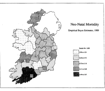
T h e p a t t e r n o f e m p i r i c a l Bayes estimates is, as one m i g h t expect, b r o a d l y s i m i l a r t o the p a t t e r n o f r a w rates (or m a x i m u m l i k e l i h o o d estimates) s h o w n i n F i g u r e 2. However, t h e r e are also some notable differences ( F i g u r e 4). I t w i l l be noted, for example, t h a t C o r k has n o w emerged as t h e area of h i g h est r i s k , o v e r t a k i n g 4 counties w i t h a m u c h s m a l l e r p o p u l a t i o n . L i k e w i s e G a l w a y , a county w i t h a large p o p u l a t i o n , has moved i n t o t h e l o w e s t r i s k category, w h i l s t L e i t r i m , a county w i t h a l o w p o p u l a t i o n , has moved f r o m a h i g h r i s k category i n t o a m e d i u m r i s k category. O v e r a l l , t h e r e i s a h i g h e r degree o f s p a t i a l a u t o c o r r e l a t i o n i n t h e d i s t r i b u t i o n o f t h e e m p i r i c a l Bayes e s t i m a t e s — i.e., t h e r e is a g r e a t e r degree o f r e g i o n a l p a t t e r n i n g i n t h e e m p i r i c a l Bayes estimates, possibly i n d i c a t i n g a r e d u c t i o n i n t h e "noise t o signal" ratio.
Figure 4: Spatial Distribution of Empirical Bayes Estimates ofNeo-Natal Mortality Rates in 1989.
estimates. However, i f i t is assumed t h a t t h e p a t t e r n of r i s k s r e m a i n s m u c h t h e same f r o m one year to t h e next, t h e n one w a y o f gauging w h i c h m e t h o d provides t h e b e t t e r e s t i m a t e s o f t h e r i s k s i n 1989 is to see w h i c h set o f estimates provides t h e b e t t e r p r e d i c t i o n o f t h e a c t u a l numbers of deaths i n 1990. T h e expected n u m b e r of deaths i n 1990 were therefore calculated u s i n g three a l t e r n a t i v e approaches:
(a) T h e expected n u m b e r o f deaths i n each county was calculated assum i n g a n e q u a l r i s k i n each area — t h i s is equivalent t o a s s u m i n g t h a t t h e r e is no systematic v a r i a t i o n i n r i s k a n d t h a t t h e observed p a t t e r n of neo-natal m o r t a l i t y s i m p l y reflects stochastic variations;
assuming t h e r e l a t i v e r i s k s i n 1990 were d i s t r i b u t e d i n t h e same w a y as t h e empirical Bayes estimates i n 1989.
The n u m b e r of deaths i n each county predicted b y each m e t h o d was t h e n compared w i t h the actual n u m b e r o f deaths i n 1990. The performance of each m e t h o d is s u m m a r i s e d b y c a l c u l a t i n g t h e m e a n o f t h e absolute differences b e t w e e n t h e observed a n d expected n u m b e r of deaths i n each a r e a .3 T h e results are shown i n Table 3.
Table 3: Relative Accuracy of Three Predictions ofNeo-natal Deaths in 1990 Mean Absolute Error
Method 1 — Equal Risk 2.56
Method 2 — Maximum Likelihood Estimates 2.75
Method 3 — Empirical Bayes Estimates 2.45
Comparison of the f i r s t t w o methods r a t h e r s u r p r i s i n g l y indicates t h a t one could p r e d i c t t h e n u m b e r of deaths i n each county i n 1990 more accurately a s s u m i n g t h a t a l l counties h a d exactly t h e same r i s k r a t h e r t h a n u s i n g t h e i n f o r m a t i o n on t h e m a x i m u m l i k e l i h o o d estimates o f t h e neo-natal rates i n 1989 as a guide. T h i s w o u l d suggest t h a t most of t h e observed v a r i a t i o n s i n neo-natal rates i n 1989 are a c t u a l l y stochastic noise generated by t h e s m a l l n u m b e r s p r o b l e m , r a t h e r t h a n a r e l i a b l e i n d i c a t i o n o f v a r i a t i o n s i n t h e u n d e r l y i n g r i s k .
T h e 1989 e m p i r i c a l Bayes estimates, i n contrast, p r o v i d e a b e t t e r pre d i c t i o n o f t h e 1990 r a t e s t h a n t h e m e t h o d a s s u m i n g e q u a l r i s k . T h e i m p r o v e m e n t is a d m i t t e d l y q u i t e s m a l l . However, i f one examines F i g u r e 3, i t w i l l be noted t h a t most o f t h e e m p i r i c a l Bayes estimates have been " s h r u n k " t o a value close to t h e n a t i o n a l m e a n (or, t o p u t i t another w a y , close t o t h e values w h i c h w o u l d p e r t a i n u n d e r a n assumption o f equal r i s k ) . T h e "signal" detected by t h e e m p i r i c a l Bayes estimates is s t i l l v e r y weak, b u t t h e fact t h a t i t produces a n i m p r o v e m e n t i n t h e accuracy of t h e predictions suggests t h a t t h e technique is i n fact successfully detecting r e a l ( a n d persistent) v a r i a t i o n s i n t h e u n d e r l y i n g r i s k .
Case Study 2 : Female Cancer Mortality
Female deaths from m a l i g n a n t neoplasms are examined i n t h e second case study. T h i s w o u l d appear, i n some respects, to provide a less d i f f i c u l t c h a l lenge t h a n neo-natal m o r t a l i t y . T h e r e were a t o t a l o f 3,481 deaths amongst
w o m e n f r o m cancer i n 1989, compared w i t h o n l y 249 neo-natal deaths, so one m i g h t assume t h a t t h e s m a l l n u m b e r s problem w o u l d be less pronounced a n d t h a t t h e u n d e r l y i n g s p a t i a l v a r i a t i o n s i n r i s k w o u l d be revealed by con v e n t i o n a l m a x i m u m l i k e l i h o o d methods. However, cancer m o r t a l i t y provides a more d i f f i c u l t challenge i n other respects. Cancer is probably n o t a single disease b u t a f a m i l y o f diseases w i t h d i f f e r e n t aetiologies a n d possibly d i f f e r e n t geographies, m a k i n g i t more d i f f i c u l t to i d e n t i f y r e g u l a r s p a t i a l v a r i a t i o n s i n r i s k . Also, the r i s k o f m o r t a l i t y f r o m cancer increases w i t h age. T h i s creates t w o complications. F i r s t , a h i g h m o r t a l i t y r a t e i n a p a r t i c u l a r area amongst t h e elderly does n o t necessarily i n d i c a t e a h e a l t h concern: i t could i n d i c a t e t h a t a h i g h e r p r o p o r t i o n o f w o m e n are l i v i n g t o a n o l d age before e v e n t u a l l y succumbing to cancer (i.e., i t could i n a paradoxical sort o f w a y i n d i c a t e l o w r i s k ) . Second, i t becomes necessary to t a k e account o f v a r i a t i o n s i n age composition between areas, due t o t h e fact t h a t a n area h a v i n g a n e l d e r l y p o p u l a t i o n w o u l d be expected, a l l other t h i n g s being equal, to experience more fatalities from cancer t h a n a n area w i t h a younger popu l a t i o n — i.e., t h e crude d e a t h r a t e does n o t necessarily provide a r e l i a b l e i n d i c a t i o n o f t h e u n d e r l y i n g r i s k .
T h e f i r s t p r o b l e m is c i r c u m v e n t e d i n t h i s s t u d y by c o n s i d e r i n g o n l y "premature" deaths (defined here as deaths below the age o f 65). T h i s reduces t h e n u m b e r o f deaths under consideration from 3,481 to 1,061. T h i s solves t h e i n t e r p r e t a t i o n problems caused b y deaths amongst t h e elderly, b u t intensifies t h e difficulties caused b y the s m a l l n u m b e r s problem. The second problem is n o r m a l l y resolved by c a l c u l a t i n g either age-specific rates for each age-group or b y c a l c u l a t i n g a w e i g h t e d age-standardised index. C l a y t o n a n d K a l d o r (1987) o u t l i n e a procedure for e x t e n d i n g t h e simple e m p i r i c a l Bayes m e t h o d used i n t h e f i r s t case s t u d y t o t a k e account of v a r i a t i o n s i n age composition. T h i s m a y be r e g a r d e d as a n e m p i r i c a l Bayes e q u i v a l e n t o f a n i n d i r e c t l y s t a n a r d i s e d r a t e . T h e procedure requires a r e l a t i v e r i s k t o be e s t i m a t e d for each age group i n a d d i t i o n t o t h e e s t i m a t i o n of a r e l a t i v e r i s k for each area. T h e t w o sets of r e l a t i v e r i s k s are estimated simultaneously u s i n g a n i t e r a t i v e approach.
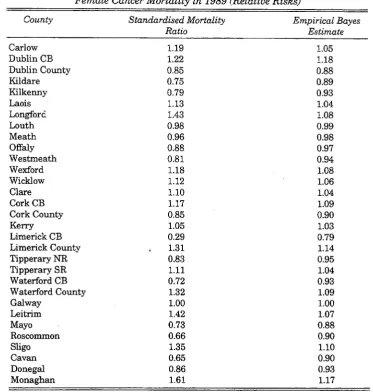
F i g u r e 5 g r a p h s t h e s t a n d a r d i s e d m o r t a l i t y r a t i o ( c a l c u l a t e d b y t h e i n d i r e c t m e t h o d ) for each area against t h e female p o p u l a t i o n aged less t h a n 65 y e a r s .4 I t also shows the e m p i r i c a l Bayes estimate o f t h e r e l a t i v e r i s k for each area. A s before, t h e e m p i r i c a l Bayes e s t i m a t e s for each a r e a are
i n v a r i a b l y closer t o t h e overall m e a n t h a n t h e corresponding standardised m o r t a l i t y r a t i o . The largest differences are generally i n t h e areas w i t h t h e smallest populations. T h e standardised m o r t a l i t y r a t i o s range from a l o w o f 0.29 ( L i m e r i c k C B ) to a h i g h o f 1.61 ( M o n a g h a n ) , whereas values for t h e e m p i r i c a l Bayes estimates range from a l o w of 0.79 ( L i m e r i c k C B ) t o a h i g h o f 1.18 for D u b l i n C B (Table 4). The e m p i r i c a l Bayes estimates i n t u i t i v e l y seem more plausible. The L i m e r i c k values, for example, are based o n only 5 deaths i n 1989, w h e r e a s t h e r e were 19 d e a t h s i n L i m e r i c k i n 1990, suggest i n g t h a t t h e exceptionally low n u m b e r of deaths ( a n d correspondingly l o w standardised m o r t a l i t y r a t i o ) i n 1989 m a y have been a freak occurrence.
1.8
1.6
1.4 +
2 1.2 2
> i
-Pi "•' 0.8 0.6
0.4
-0.2
8 ©
©
Indirect SMRs
Empirical Bayes
©
r© © ©
©
50000 100000 150000 200000
Females Aged <65 Years
250000
Figure 5: Standardised Mortality Ratios and Empirical Bayes Estimates of Relative Risk For Female Cancer Deaths in 1989 Graphed Against the Population at Risk.
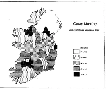
T h e s p a t i a l d i s t r i b u t i o n of t h e standardised m o r t a l i t y r a t i o s is s h o w n i n F i g u r e 6. T h e s p a t i a l d i s t r i b u t i o n of t h e e m p i r i c a l Bayes estimates is s h o w n i n F i g u r e 7. N e i t h e r m a p e x h i b i t s a c o n v i n c i n g degree o f s p a t i a l order, suggesting e i t h e r t h a t more data m a y be r e q u i r e d to i d e n t i f y t h e u n d e r l y i n g s p a t i a l r e g u l a r i t i e s i n r i s k or else t h a t such r e g u l a r i t i e s do n o t i n fact exist for cancer t a k e n as a whole.
Table 4: Standardised Mortality Ratios and Empirical Bayes Estimates of Female Cancer Mortality in 1989 (Relative Risks)
County Standardised Mortality Empirical Bayes
Ratio Estimate
Carlow 1.19 1.05
Dublin CB 1.22 1.18
Dublin County 0.85 0.88
Kildare 0.75 0.89
Kilkenny 0.79 0.93
Laois 1.13 1.04
Longford 1.43 1.08
Louth 0.98 0.99
Meath 0.96 0.98
Offaly 0.88 0.97
Westmeath 0.81 0.94
Wexford 1.18 1.08
Wicklow 1.12 1.06
Clare 1.10 1.04
Cork CB 1.17 1.09
Cork County 0.85 0.90
Kerry 1.05 1.03
Limerick CB 0.29 0.79
Limerick County 1.31 1.14
Tipperary NR 0.83 0.95
Tipperary SR 1.11 1.04
Waterford CB 0.72 0.93
Waterford County 1.32 1.09
Galway 1.00 1.00
Leitrim 1.42 1.07
Mayo 0.73 0.88
Roscommon 0.66 0.90
Sligo 1.35 1.10
Cavan 0.65 0.90
Donegal 0.86 0.93
Monaghan 1.61 1.17
results i n s i m i l a r conclusions t o the previous case study (Table 5). A s before, t h e conventional m e t h o d produces poorer predictions t h a n t h e assumption of no systematic v a r i a t i o n i n r i s k between areas, h i g h l i g h t i n g t h e v u l n e r a b i l i t y of c o n v e n t i o n a l indices t o stochastic f l u c t u a t i o n s .5 However, t h e e m p i r i c a l Bayes estimates represent a s u b s t a n t i a l i m p r o v e m e n t over each of t h e other t w o methods.
Figure 6: Spatial Distribution of Stanardised Mortality Ratios for Female Cancer Deaths in 1989.
Table 5: Relative Accuracy of Three Predictions of Female Cancer Deaths in 1990
Mean Absolute Error
Method 1 — Equal Risk 6.35
Method 2 — Standardised Mortality Ratios 6.46
Figure 7: Spatial Distribution of Empirical Bayes Estimates of Relative Risk for Female Cancer Deaths in 1989.
V D I S C U S S I O N
of t h e m a x i m u m l i k e l i h o o d estimates i n these tests h i g h l i g h t s j u s t h o w serious the s m a l l numbers problem can be.
These f i n d i n g s suggest t h a t , where possible, e m p i r i c a l Bayes e s t i m a t e s should be used as a n a l t e r n a t i v e (or at least as a supplement) to conventional m a x i m u m l i k e l i h o o d estimates of disease r i s k . A l t h o u g h t h e present paper discusses t h e p r o b l e m of e s t i m a t i n g disease r i s k i n t h e context o f disease m a p p i n g , s i m i l a r a r g u m e n t s a p p l y to estimates of disease r i s k for o t h e r purposes (e.g., i n v e s t i g a t i o n s o f t e m p o r a l t r e n d s ) . L i k e w i s e , B a y e s i a n approaches m a y provide i m p r o v e d estimates for non-medical data. Cressie (1995), for example, outlines methods for e s t i m a t i n g t h e t r u e rates for socio economic v a r i a b l e s (e.g., u n e m p l o y m e n t rates, per c a p i t a incomes) f r o m "noisy" observed data, p a y i n g p a r t i c u l a r a t t e n t i o n to the p r o b l e m of e s t i m a t i n g census undercounts. The major difference between these s i t u a t i o n s a n d t h e m e d i c a l examples discussed above is t h a t t h e source o f u n c e r t a i n t y is assumed t o be m e a s u r e m e n t errors r a t h e r t h a n stochastic v a r i a b i l i t y : t h e u n c e r t a i n t y is therefore assumed t o be Gaussian (i.e., N o r m a l l y d i s t r i b u t e d ) r a t h e r t h a n conforming to a Poisson process.
T h e case studies r e p o r t e d above assume c o m p a r a t i v e l y simple models. I t s h o u l d perhaps be noted, however, t h a t more complex models have been proposed to t a k e account of s p a t i a l structures, such as autocorrelation and/or r e g i o n a l i s a t i o n (e.g., C l a y t o n a n d K a l d o r , 1987; M a r s h a l l , 1991). I n o t h e r w o r d s , t h e y a l l o w one t o b u i l d a n a s s u m p t i o n i n t o t h e e m p i r i c a l Bayes estimates t h a t the disease r i s k s w i l l e x h i b i t s p a t i a l autocorrelation (i.e., t h a t a d j o i n i n g areas w i l l t e n d to have more s i m i l a r r i s k s t h a n d i s t a n t areas) or t h a t areas w i t h i n defined regions w i l l t e n d t o have s i m i l a r r i s k s . Several authors have also suggested ways to incorporate covariates i n t o t h e models to t a k e account of suspected r i s k factors, such as p o l l u t i o n or u r b a n i s a t i o n (e.g., T s u t a k a w a et al., 1985; C l a y t o n a n d K a l d o r , 1987; H e i s t e r k a m p et al., 1993; Cressie, 1995). The usefulness of these enhancements clearly depends u p o n w h e t h e r t h e objective is to examine t h e data t o identify e m p i r i c a l r e g u l a r i t i e s or, h a v i n g determined t h a t these regularities exist, to model the data t o m a k e more accurate predictions, possibly for p l a n n i n g purposes.
REFERENCES
BAILEY, T.C., and A.C. GATRELL, 1995. Interactive Spatial Data Analysis, London: Longman.
CHOYNOWSKI, M . , 1959. "Maps Based on Probabilities", Journal of the American Statistical Association, Vol. 54, pp. 585-588.
CLAYTON, D., and J. KALDOR, 1987. "Empirical Bayes Estimates of Age-standard ized Relative Risks for Use i n Disease Mapping", Biometrics, Vol. 43, pp. 671-681. CONGDON, P. 1990. "Issues i n the Analysis of Small Area Mortality", Urban Studies,
CRESSIE, N . , 1993. "Regional Mapping of Incidence Rates Using Spatial Bayesian Models", Medical Care, Vol. 31, No. 5, Supplement, YS60-YS65.
CRESSIE, N . , 1995. "Bayesian Smoothing of Rates i n Small Geographic Areas", Journal of Regional Science, Vol. 35, No. 4, pp. 659-673.
DAWSON, D.F., 1911. "The Relation Between the Geographical Distribution of Insanity and that of Certain Social and Other Conditions i n Ireland", Journal of Mental Science, Vol. 57, pp. 571-597.
DIEHR, P., 1984. "Small Area Statistics: Large Statistical Problems", American Journal of Public Health, Vol. 74, pp. 313-314.
DUNCAN, C , K. JONES, and G. MOON, 1993. "Do Places Matter? A Multi-level Analysis of Regional Variations i n Health-related Behaviour i n Britain", Social Science and Medicine, Vol. 37, pp. 725-733.
GIGGS, J.A., D.S. EBDON, and J.B. BOURKE, 1980. "The Epidemiology of Primary Acute Pancreatis i n the Nottingham Defined Population Area", Transactions of the Institute of British Geographers, Vol. 5, pp. 229-242.
HEISTERKAMP, S.H., G. DOORNBOS, and M . GANKEMA, 1993. "Disease Mapping using Empirical Bayes and Bayes Methods on M o r t a l i t y Statistics i n The Netherlands", Statistics in Medicine, Vol. 12, pp. 1,895-1,913.
HOWELL, F., M . O'MAHONY, J. D E V L I N , O. O'REILLY, C. BUTTANSHAW, 1993. "A Geographical Distribution of Mortality and Deprivation", Irish Medical Journal, Vol. 86, pp. 96-99.
IVERSON, G.D., 1984. Bayesian Statistical Inference, Beverly Hills: Sage Publi cations.
JOHNSON, Z., and P. DACK, 1989. "Small Area Mortality Patterns", Irish Medical Journal, Vol. 82, pp. 105-108.
KALDOR, J., and D. CLAYTON, 1989. "Role of Advanced Statistical Techniques i n Cancer Mapping", Recent Results in Cancer Research, Vol. 114, pp. 87-98.
K I N G , P.E., 1979. "Problems of Spatial Analysis i n Geographic Epidemiology", Social Science and Medicine, Vol. 13D, pp. 249-252.
LANGFORD, I . H . , 1994. "Using Empirical Bayes Estimates i n the Geographical Analysis of Disease Risk", Area, Vol. 26, pp. 142-149.
M A N T O N , K.G., E. STALLARD, M.A. WOODBURY, W.B. RIGGAN, J.P. CREASON, and T.J. MASON, 1987. "Statistically Adjusted Estimates of Geographic Mortality Profiles", Journal of the National Cancer Institute, Vol. 78, pp. 805-815.
MARSHALL, R.J., 1991. "Mapping Disease and Mortality Rates Using Empirical Bayes Estimators", Applied Statistics, Vol. 40, pp. 283-294.
M I Y A W A K I , N . , and S.C. C H E N S.C., 1981. "A Statistical Consideration on the Mapping of Disease", Social Science and Medicine, Vol. 15, D, pp. 93-101.
MONMONIER, M . , 1991. How To Lie With Maps, Chicago: University of Chicago Press.
PRESSAT, R., 1978. Statistical Demography, London: Methuen.
PRINGLE, D.G., 1983. "Mortality, Cause of Death and Social Class i n the Belfast Urban Area", Ecology of Disease, Vol. 2, pp. 1-8.
PRINGLE, D.G., 1986. "Premature Mortality i n the Republic of Ireland, 1971-1981", Irish Geography, Vol. 19, pp. 33-40.
STONE, R.A., 1988, "Investigations of Excess Environmental Risks Around Putative Sources: Statistical Problems and a Proposed Test", Statistics in Medicine, Vol. 7, pp. 649-660.
TSUTAKAWA, R.K., G.L. SHOOP, and C.J. MARIENFELD, 1985. "Empirical Bayes Estimation of Cancer Mortality Rates", Statistics in Medicine, Vol. 4, pp. 201-212. TSUTAKAWA, R.K., 1988. "Mixed Model for Analyzing Geographic Variability i n
Mortality Rates", Journal of the American Statistical Association, Vol. 83, No. 401, pp. 37-42.