Fast Statistical Parsing with Parallel Multiple Context-Free Grammars
Krasimir Angelov and Peter Ljungl¨of
University of Gothenburg and Chalmers University of Technology G¨oteborg, Sweden
krasimir@chalmers.se peter.ljunglof@cse.gu.se
Abstract
We present an algorithm for incremental statistical parsing with Parallel Multiple Context-Free Grammars (PMCFG). This is an extension of the algorithm by An-gelov (2009) to which we added statisti-cal ranking. We show that the new al-gorithm is several times faster than other statistical PMCFG parsing algorithms on real-sized grammars. At the same time the algorithm is more general since it supports non-binarized and non-linear grammars. We also show that if we make the search heuristics non-admissible, the pars-ing speed improves even further, at the risk of returning sub-optimal solutions. 1 Introduction
In this paper we present an algorithm for incre-mental parsing using Parallel Multiple Context-Free Grammars (PMCFG) (Seki et al., 1991). This is a non context-free formalism allowing disconti-nuity and crossing dependencies, while remaining with polynomial parsing complexity.
The algorithm is an extension of the algorithm by Angelov (2009; 2011) which adds statistical ranking. This is a top-down algorithm, shown by Ljungl¨of (2012) to be similar to other top-down al-gorithms (Burden and Ljungl¨of, 2005; Kanazawa, 2008; Kallmeyer and Maier, 2009). None of the other top-down algorithms are statistical.
The only statistical PMCFG parsing algorithms (Kato et al., 2006; Kallmeyer and Maier, 2013; Maier et al., 2012) all use bottom-up parsing strategies. Furthermore, they require the gram-mar to be binarized and linear, which means that they only support linear context-free rewriting sys-tems (LCFRS). In contrast, our algorithm natu-rally supports the full power of PMCFG. By lift-ing these restrictions, we make it possible to
ex-periment with novel grammar induction methods (Maier, 2013) and to use statistical disambiguation for hand-crafted grammars (Angelov, 2011).
By extending the algorithm with a statistical model, we allow the parser to explore only parts of the search space, when only the most proba-ble parse tree is needed. Our cost estimation is similar to the estimation for the Viterbi probabil-ity as in Stolcke (1995), except that we have to take into account that our grammar is not context-free. The estimation is both admissible and mono-tonic (Klein and Manning, 2003) which guaran-tees that we always find a tree whose probability is the global maximum.
We also describe a variant with a non-admissible estimation, which further improves the efficiency of the parser at the risk of returning a suboptimal parse tree.
We start with a formal definition of a weighted PMCFG in Section 2, and we continue with a pre-sentation of our algorithm by means of a weighted deduction system in Section 3. In Section 4, we prove that our estimations are admissible and monotonic. In Section 5 we calculate an esti-mate for the minimal inside probability for every category, and in Section 6 we discuss the non-admissible heuristics. Sections 7 and 8 describe the implementation and our evaluation, and the fi-nal Section 9 concludes the paper.
2 PMCFG definition
Our definition of weighted PMCFG (Definition 1) is the same as the one used by Angelov (2009; 2011), except that we extend it with weights for the productions. This definition is also similar to Kato et al (2006), with the small difference that we allow non-linear functions.
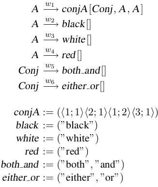
As an illustration for PMCFG parsing, we use a simple grammar (Figure 1) which can generate phrases like “both black and white” and“either red or white” but rejects the incorrect
Definition 1
A parallel multiple context-free grammar is a tuple
G= (N, T, F, P, S, d, di, r, a)where:
• N is a finite set of categories and a positive in-tegerd(A) called dimension is given for each
A∈N.
• Tis a finite set of terminal symbols which is dis-joint withN.
• Fis a finite set of functions where the aritya(f)
and the dimensionsr(f) anddi(f) (1 ≤ i ≤
a(f)) are given for every f ∈ F. For every positive integerd,(T∗)ddenote the set of alld -tuples of strings overT. Each functionf ∈ F
is a total mapping from(T∗)d1(f)×(T∗)d2(f)× · · · ×(T∗)da(f)(f)to(T∗)r(f), defined as:
f := (α1, α2, . . . , αr(f))
Here αi is a sequence of terminals and hk;li pairs, where1 ≤k ≤ a(f)is called argument index and1 ≤ l ≤ dk(f)is called constituent index.
• P is a finite set of productions of the form:
A−→w f[A1, A2, . . . , Aa(f)]
where A ∈ N is called result category,
A1, A2, . . . , Aa(f) ∈ N are called argument categories, f ∈ F is the function symbol and
w > 0 is a weight. For the production to be well formed the conditionsdi(f) =d(Ai) (1≤
i≤a(f))andr(f) =d(A)must hold. • Sis the start category andd(S) = 1.
tionsboth-orandeither-and. We avoid these com-binations by coupling the right pairs of words in a single function, i.e. we have the abstract conjunc-tionsboth and andeither or which are linearized as discontinuous phrases. The phrase insertion it-self is done in the definition ofconjA. It takes the conjunction as its first argument, and it usesh1; 1i
and h1; 2i to insert the first and the second con-stituent of the argument at the right places in the complete phrase.
A tree of function applications that yelds a com-plete phrase is the parse tree for the phrase. For instance, the phrase“both red and either black or white”is represented by the tree:
(conjA both and red
(conjA either or black white))
A −→w1 conjA[Conj,A,A]
A −→w2 black[]
A −→w3 white[]
A −→w4 red[]
Conj −→w5 both and[]
Conj −→w6 either or[]
conjA:= (h1; 1ih2; 1ih1; 2ih3; 1i)
black := (”black”)
white := (”white”)
red := (”red”)
both and := (”both”,”and”)
[image:2.595.334.497.75.268.2]either or:= (”either”,”or”)
Figure 1: Example Grammar
The weight of a tree is the sum of the weights for all functions that are used in it. In this case the weight for the example isw1+w5+w4+w1+w6+
w2+w3. If there are ambiguities in the sentence,
the algorithm described in Section 3 always finds a tree which minimizes the weight.
Usually the weights for the productions are log-arithmic probabilities, i.e. the weight of the pro-ductionA→f[B]~ is:
w=−logP(A→f[B~]|A)
where P(A → f[B]~ | A) is the probability to choose this production when the result category is fixed. In this case the probabilities for all produc-tions with the same result category sum to one:
X
A−→w f[B~]∈P
e−w= 1
However, the parsing algorithm does not depend on the probabilistic interpretation of the weights, so the same algorithm can be used with any other kind of weights.
3 Deduction System
We define the algorithm as weighted deduction system (Nederhof, 2003) which generalizes An-gelov’s system.
can be exemplified with the grammar in Fig-ure 1, where there are two productions for cat-egory Conj. Given the phrase “both black and white”, after accepting the token both, only the production Conj −→w5 both and[] can be applied
for parsing the second part of the conjunction. This is achieved by generating a new category
Conj2which has just a single production:
Conj2 −→w5 both and[] (1)
The parsing algorithm is basically an extension of Earley’s (1970) algorithm, except that the parse items in the chart also keep track of the categories for the arguments. In the particular case, the cor-responding chart item will be updated to point to
Conj2 instead ofConj. This guarantees that only
andwill be accepted as a second constituent after seeing that the first constituent isboth.
Now since the set of productions is dynamic, the parser must keep three kinds of items in the chart, instead of two as in the Earley algorithm:
Productions The parser maintains a dynamic set with all productions that are derived during the parsing. The initial state is populated with the pro-ductions from the setP in the grammar.
Active Items The active items play the same role as the active items in the Earley algorithm. They have the form:
[kjA−→w f[B];~ l:α•β;wi;wo]
and represent the fact that a constituentlof a cat-egoryAhas been partially recognized from posi-tion j tok in the sentence. Here A −→w f[B]~ is the production and the concatenationαβis the se-quence of terminals andhk;ripairs which defines the l-th constituent of function f. The dot • be-tweenαandβseparates the part of the constituent that is already recognized from the part which is still pending. Finallywiandwoare the inside and
outside weights for the item.
Passive Items The passive items are of the form:
[kjA;l; ˆA]
and state that a constituent with indexlfrom cate-goryAwas recognized from positionjto position kin the sentence. As a consequence the parser has created a new categoryAˆ. The set of productions derived forAˆcompactly records all possible ways to parse thej−kfragment.
3.1 Inside and outside weights
The inside weightwiand the outside weightwoin
the active items deserve more attention since this is the only difference compared to Angelov (2009; 2011). When the item is complete, it will yield the forest of all trees that derive the sub-string cov-ered by the item. For example, when the first con-stituent for category Conj is completely parsed, the forest will contain the single production in (1). The inside weight for the active item is the cur-rently best known estimation for the lowest weight of a tree in the forest. The trees yielded by the item do not cover the whole sentence however. Instead, they will become part of larger trees that cover the whole sentence. The outside weight is the esti-mation for the lowest weight for an extension of a tree to a full tree. The sumwi+woestimates the
weight of the full tree.
Before turning to the deduction rules we also need a notation for the lowest possible weight for a tree of a given category. IfA ∈N is a category thenwAwill denote the lowest weight that a tree of
categoryAcan have. For convenience, we also use wB~ as a notation for the sumPiwBiof the weight of all categories in the vector B~. If the category Ais defined in the grammar then we assume that the weight is precomputed as described in Section 5. When the parser creates the category, it will compute the weight dynamically.
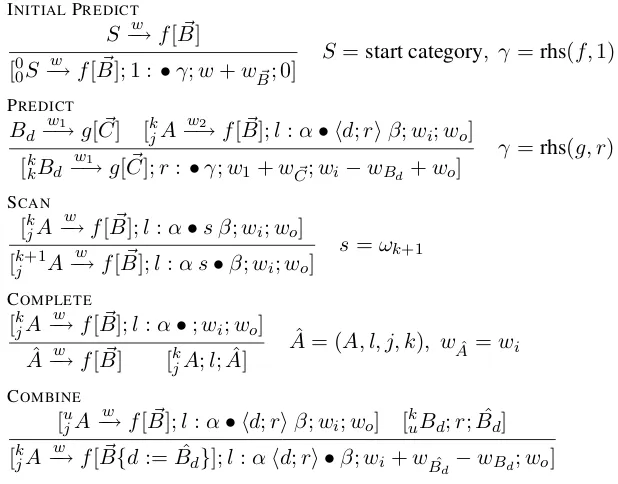
3.2 Deduction rules
The deduction rules are shown in Figure 2. Here the assumption is that the active items are pro-cessed in the order of increasingwi+wo weight.
In the actual implementation we put all active items in a priority queue and we always take first the item with the lowest weight. We never throw away items but the processing of items with very high weight might be delayed indefinitely or they may never be processed if the best tree is found before that. Furthermore, we think of the deduc-tion system as a way do derive a set of items, but in our case we ignore the weights when we consider whether two active items are the same. In this way, every item is derived only once and the weights for the active items are computed from the weights of the first antecedents that led to its derivation.
Finally, we use two more notations in the rules: rhs(g, r)denotes constituent with indexrin func-tion g; and ωk denotes the k-th token in the
INITIALPREDICT
S−→w f[B]~
[00S −→w f[B]; 1 :~ •γ;w+wB~; 0] S=start category, γ=rhs(f,1)
PREDICT
Bd−→w1 g[~C] [kjA−→w2 f[B];~ l:α• hd;riβ;wi;wo]
[k
kBd−→w1 g[~C];r:•γ;w1+wC~;wi−wBd+wo]
γ =rhs(g, r)
SCAN
[k
jA−→w f[B];~ l:α•s β;wi;wo]
[k+1
j A−→w f[B];~ l:α s•β;wi;wo] s=ωk+1
COMPLETE
[kjA−→w f[B];~ l:α•;wi;wo]
ˆ
A−→w f[B]~ [kjA;l; ˆA] Aˆ= (A, l, j, k), wAˆ =wi COMBINE
[u
jA−→w f[B];~ l:α• hd;riβ;wi;wo] [kuBd;r; ˆBd]
[k
[image:4.595.143.452.73.315.2]jA−→w f[B~{d:= ˆBd}];l:αhd;ri •β;wi+wBˆd−wBd;wo]
Figure 2: Deduction Rules
The first rule on Figure 2 isINITIALPREDICTand
here we predict the initial active items from the productions for the start category S. Since this is the start category, we set the outside weight to zero. The inside weight is equal to the sum of the weightw for the production and the lowest pos-sible weight wB~ for the vector of arguments B~.
The reason is that despite that we do not know the weight for the final tree yet, it cannot be lower than w+wB~ sincewB~ is the lowest possible weight for
the arguments of functionf.
The interaction between inside and outside weights is more interesting in the PREDICT rule.
Here we have an item where the dot is beforehd;ri
and from this we must predict one item for each productionBd−→w1 g[~C]of categoryBd. The
in-side weight for the new item isw1 +wC~ for the
same reasons as for the INITIALPREDICT rule. The
outside weight however is not zero because the new item is predicted from another item. The in-side weight for the active item in the antecedents is now part of the outside weight of the new item. We just have to subtractwBdfromwibecause the new item is going to produce a new tree which will replace thed-th argument off. For this reason the estimation for the outside weight iswi−wBd+wo, where we also added the outside weight for the an-tecedent item.
In the SCAN rule, we just move the dot past a
token, if it matches the current tokenωk+1. Both
the inside and the outside weights are passed un-touched from the antecedent to the consequent.
In theCOMPLETErule, we have an item where the
dot has reached the end of the constituent. Here we generate a new categoryAˆwhich is unique for the combination(A, l, j, k), and we derive the produc-tionAˆ−→w f[B]~ for it. We set the weightwAˆforAˆ
to be equal towi and in Section 4, we will prove
that this is indeed the lowest weight for a tree of categoryAˆ.
In the last ruleCOMBINE, we combine an active
item with a passive item. The outside weightwo
for the new active item remains the same. How-ever, we must update the inside weight since we have replaced the d-th argument in B~ with the newly generated categoryBˆd. The new weight is
wi+wBˆd−wBd, i.e. we add the weight for the new category and we subtract the weight for the previous categoryBd.
Now for the correctness of the weights we must prove that the estimations are both admissible and monotonic.
4 Admissibility and Monotonicity
We will first prove that the weights grow mono-tonically, i.e. if we derive one active item from another then the sumwi+wofor the new item is
item. PREDICTandCOMBINEare the only two rules
with an active item both in the antecedents and in the consequents.
Note that in PREDICT we choose one particular
production for category Bd. We know that the
lowest possible weight of a tree of this category is wBd. If we restrict the set of trees to those that not only have the same category Bdbut also
use the same productionBd −→w1 g[~C]on the top
level, then the best weight for such a tree will be w1+wC~. According to the definition ofwBd, it must follow that:
w1+wC~ ≥wBd From this we can trivially derive that:
(w1+wC~) + (wi−wBd+wo)≥wi+wo which is the monotonicity condition for rule
PREDICT. Similarly in ruleCOMBINE, the condition:
wBˆd≥wBd
must hold because the forest of trees forBˆdis
in-cluded in the forest forBd. From this we conclude
the monotonicity condition:
(wi+wBˆd−wBd) +wo≥wi+wo The last two inequalities are valid only if we can correctly compute wBˆd for a dynamically
gener-ated categoryBˆd. This happens in ruleCOMPLETE,
where we have a complete active item with a cor-rectly computed inside weightwi. Since we
pro-cess the active items in the order of increasing wi+wo weight and since we createAˆwhen we
find the first complete item for category A, it is guaranteed that at this point we have an item with minimal wi +wo value. Furthermore, all items
with the same result categoryAand the same start positionj must have the same outside weight. It follows that when we create Aˆ we actually do it from an active item with minimal inside weight wi. This means that it is safe to assign thatwAˆ =
wi.
It is also easy to see that the estimation is ad-missible. The only places where we use estima-tions for the unseen parts of the sentence is in the rules INITIALPREDICT and PREDICT where we use
the weightswB~ andwC~ which may include
com-ponents corresponding to function argument that are not seen yet. However by definition it is not possible to build a tree with weight lower than the weight for the category. This means that the esti-mation is always admissible.
5 Initial Estimation
The minimal weight for a dynamically created cat-egory is computed by the parser, but we must ini-tialize the weights for the categories that are de-fined in the grammar. The easiest way is to just set all weights to zero, and this is safe since the weights for the predefined categories are used only as estimations for the yet unseen parts of the sen-tence. Essentially this gives us a statistical parser which performs Dijkstra search in the space of all parse trees. Any other reasonable weight assign-ment will give us an A∗ algorithm (Hart et al.,
1968).
In general it is possible to devise different heuristics which will give us different improve-ments in the parsing time. In our current im-plementation of the parser we use a weight as-signment which considers only the already known probabilities for the productions in the grammar.
The weight for a categoryAis computed as: wA= min
A−→w f[B~]∈P(w+wB~)
Here the sumw+wB~ is the minimal weight for a tree constructed with the productionA −→w f[B]~ at the root. By taking the minimum over all pro-ductions for A, we get the corresponding weight wA. This is a recursive equation since its
right-hand side contains the valuewB~ which depends on
the weights for the categories inB~. It might hap-pen that there are mutually dehap-pendent categories which will lead to a recursion in the equation.
The solution is found with iterative assignments until a fixed point is reached. In the beginning we assignwA= 0for all categories. After that we
re-compute the new weights with the equation above until we reach a fixed point.
6 Non-admissible heuristics
This suggests that when we compare the weights of items with different end positions, then we must take into account the weight that will be accumu-lated by the item that ends earlier until the two items align at the same end position.
We use the following heuristic to estimate the difference. The first time when we extend an item from positionito positioni+ 1, we record the weight incrementw∆(i+ 1)for that position.
The increment w∆ is the difference between the
weights for the best active item reaching position i+ 1and the best active item reaching positioni. From now on when we compare the weights for two items xj andxk, with end positionsj andk
respectively (j < k), then we always add to the scorewxjof the first item a fraction of the sum of the increments for the positions betweenj andk. In other words, instead of usingwxj when com-paring withwxk, we use
wxj+h·
X
j<i≤k
w∆(i)
We call the constanth∈[0,1]the “heuristics fac-tor”. Ifh = 0, we obtain the basic algorithm that we described earlier which is admissible and al-ways returns the best parse. However, the evalua-tion in Secevalua-tion 8.3 shows that a significant speed-up can be obtained by using larger values of h. Unfortunately, ifh > 0, we loose some accuracy and cannot guarantee that the best parse is always returned first.
Note that the heuristics does not change the completeness of the algorithm – it will succeed for all grammatical sentences and fail for all non-grammatical. But it does not guarantee that the first parse tree will be the optimal.
7 Implementation
The parser is implemented in C and is distributed as a part of the runtime system for the open-source Grammatical Framework (GF) programming lan-guage (Ranta, 2011).1 Although the primary ap-plication of the runtime system is to run GF appli-cations, it is not specific to one formalism, and it can serve as an execution platform for other frame-works where natural language parsing and gener-ation is needed.
The GF system is distributed with a library of manually authored resource grammars (Ranta,
1http://www.grammaticalframework.org/
2009) for over 25 languages, which are used as a resource for deriving domain specific grammars. Adding a big lexicon to the resource grammar re-sults in a highly ambiguous grammar, which can give rise to millions of trees even for moderately complex sentences. Previously, the GF system has not been able to parse with such ambiguous gram-mars, but with our statistical algorithm it is now feasible.
8 Evaluation
We did an initial evaluation on the GF English re-source grammar augmented with a large-coverage lexicon of 40 000 lemmas taken from the Oxford Advanced Learner’s Dictionary (Mitton, 1986). In total the grammar has 44 000 productions. The rule weights were trained from a version of the Penn Treebank (Marcus et al., 1993) which was converted to trees compatible with the grammar.
The trained grammar was tested on Penn Tree-bank sentences of length up to 35 tokens, and the parsing times were at most 7 seconds per sentence. This initial test was run on a computer with a 2.4 GHz Intel Core i5 processor with 8 GB RAM. This result was very encouraging, given the complexity of the grammar, so we decided to do a larger test and compare with an existing state-of-the-art sta-tistical PMCFG parser.
Rparse (Kallmeyer and Maier, 2013) is a an-other state-of-the-art training and parsing system for PMCFG.2It is written in Java and developed at the Universities of T¨ubingen and D¨usseldorf, Ger-many. Rparse can be used for training probabilis-tic PMCFGs from discontinuous treebanks. It can also be used for parsing new sentences with the trained grammars.
In our evaluation we used Rparse to extract PM-CFG grammars from the discontinuous German Tiger Treebank (Brants et al., 2002). The rea-son for using this treebank is that the extracted grammars are non-context-free, and our parser is specifically made for such grammars.
8.1 Evaluation data
In our evaluations we got the same general results regardless of the size of the grammar, so we only report the results from one of these runs.
In this particular example, we trained the gram-mar on 40 000 sentences from the Tiger Treebank with lengths up to 160 tokens. We evaluated on
Count Training sentences 40 000 Test sentences 4 607 Non-binarized grammar rules 30 863 Binarized grammar rules 26 111
Table 1: Training and testing data.
4 600 Tiger sentences, with a length of 5–60 to-kens. The exact numbers are shown in Table 1. All tests were run on a computer with a 2.3 GHz Intel Core i7 processor with 16GB RAM.
As a comparison, Maier et al (2012) train on approximately 15 000 sentences from the Negra Treebank, and only evaluate on sentences of at most 40 tokens.
8.2 Comparison with Rparse
We evaluated our parser by comparing it with Rparse’s built-in parser. Note that we are only in-terested in the efficiency of our implementation, not the coverage and accuracy of the trained gram-mar. In the comparison we used only the ad-missible heuristics, and we did confirm that the parsers produce optimal trees with exactly the same weight for the same input.
Rparse extracts grammars in two steps. First it converts the treebank into a PMCFG, and then it binarizes that grammar. The binarization pro-cess uses markovization to improve the precision and recall of the final grammar (Kallmeyer and Maier, 2013). We tested both Rparse’s standard (Kallmeyer and Maier, 2013) and its new im-proved parsing alogorithm (Maier et al., 2012). The new algorithm unfortunately works only with LCFRS grammars with a fan-out≤2 (Maier et al., 2012).
In this test we used the optimal binarization method described in Kallmeyer (2010, chapter 7.2). This was the only binarization algorithm in Rparse that produced a grammar with fan-out≤2. As can be seen in Figure 3, our parser outper-forms Rparse for all sentence lengths. For sen-tences longer than 15 tokens, the standard Rparse parser needs on average 100 times longer time than our parser. This difference increases with sentence length, suggesting that our algorithm has a better parsing complexity than Rparse.
The PGF parser also outperforms the improved Rparse parser, but the relative difference seems to stabilize on a speedup of 10–15 times.
0,01 0,1 1 10 100
[image:7.595.308.526.61.214.2]5 10 15 20 25 30 35 40 Rparse, standard Rparse, fanout ≤ 2 PGF, admissible
Figure 3: Parsing time (seconds) compared with Rparse.
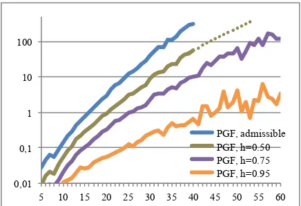
0,01 0,1 1 10 100
5 10 15 20 25 30 35 40 45 50 55 60 PGF, admissible PGF, h=0.50 PGF, h=0.75 PGF, h=0.95
Figure 4: Parsing time (seconds) with different heuristics factors.
8.3 Comparing different heuristics
In another test we compared the effect of the heuristic factorhdescribed in Section 6. We used the same training and testing data as before, and we tried four different heuristic factors: h = 0, 0.50, 0.75and0.95. As mentioned in Section 6, a factor of0gives an admissible heuristics, which means that the parser is guaranteed to return the tree with the best weight.
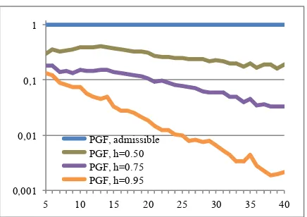
The parsing times are shown in Figure 4. As can be seen, a higher heuristics factor h gives a considerable speed-up. For 40 token sentences, h = 0.50 gives an average speedup of 5 times, whileh= 0.75is 30 times faster, andh= 0.95is almost 500 times faster than using the admissible heuristicsh= 0. This is more clearly seen in Fig-ure 5, where the parsing times are shown relative to the admissible heuristics.
[image:7.595.307.525.266.415.2]0,001 0,01 0,1 1
5 10 15 20 25 30 35 40 PGF, admissible
[image:8.595.73.291.59.213.2]PGF, h=0.50 PGF, h=0.75 PGF, h=0.95
Figure 5: Relative parsing time for different values ofh, compared to admissible heuristic.
more closely, we can see that they are not straight. The closest curves are in fact polynomial, with a degree of 4–6 depending on the parser and the value ofh.3
8.4 Non-admissibility and parsing quality
What about the loss of parsing quality when we use a non-admissible heuristics? Firstly, as men-tioned in Section 6, the parser still recognizes ex-actly the same language as defined by the gram-mar. The difference is that it is not guaranteed to return the tree with the best weight.
In our evaluation we saw that for a factor h = 0.50, 80% of the trees are optimal, and only 3% of the trees have a weight more than 5% from the optimal weight. The performance gradually gets worse for higherh, and withh= 0.95almost 10% of the trees have a weight more than 20% from the optimum.
These numbers only show how the parsing qual-ity degrades relative to the grammar. But since the grammar is trained from a treebank it is more interesting to evaluate how the parsing quality on the treebank sentences is affected when we use a non-admissible heuristics. Table 2 shows how the labelled precision and recall are changed with dif-ferent values forh. The evaluation was done us-ing the EVALB measure which is implemented in Rparse (Maier, 2010). As can be seen, a factor of h= 0.50only results in a f-score loss of 3 points, which is arguably not very much. On the other extreme, forh= 0.95the f-score drops 14 points.
3The exception is the standard Rparse parser, which has a
polynomial degree of 8.
Precision Recall F-score admissible 71.1 67.7 69.3 h= 0.50 68.0 64.9 66.4 h= 0.75 63.0 60.8 61.9 h= 0.95 55.1 55.6 55.3
Table 2: Parsing quality for different values ofh.
9 Discussion
The presented algorithm is an important general-ization of the classical algorithms of Earley (1970) and Stolcke (1995) for parsing with probabilistic context-free grammars to the more general formal-ism of parallel multiple context-free grammars. The algorithm has been implemented as part of the runtime for the Grammatical Framework (Ranta, 2011), but it is not limited to GF alone.
9.1 Performance
To show the universality of the algorithm, we eval-uated it on large LCFRS grammars trained from the Tiger Treebank.
Our parser is around 10–15 times faster than the latest, optimized version of the Rparse state-of-the-art parser. This improvement seems to be con-stant, which means that it can be a consequence of low-level optimizations. More important is that our algorithm does not impose any restrictions at all on the underlying PMCFG grammar. Rparse on the other hand requires that the grammar is both binarized and has a fan-out of at most 2.
By using a non-admissible heuristics, the speed improves by orders of magnitude, at the expense of parsing quality. This makes it possible to parse long sentences (more than 50 tokens) in just around a second on a standard desktop computer.
9.2 Future work
We would like to extend the algorithm to be able to use lexicalized statistical models (Collins, 2003). Furthermore, it would be interesting to develop better heuristics forA∗ search, and to investigate
[image:8.595.316.516.62.131.2]References
Krasimir Angelov. 2009. Incremental parsing with parallel multiple context-free grammars. In Pro-ceedings of EACL 2009, the 12th Conference of the European Chapter of the Association for Computa-tional Linguistics, Athens, Greece.
Krasimir Angelov. 2011. The Mechanics of the Gram-matical Framework. Ph.D. thesis, Chalmers Univer-sity of Technology, Gothenburg, Sweden.
Sabine Brants, Stefanie Dipper, Silvia Hansen, Wolf-gang Lezius, and George Smith. 2002. The TIGER treebank. InProceedings of TLT 2002, the 1st Work-shop on Treebanks and Linguistic Theories, So-zopol, Bulgaria.
H˚akan Burden and Peter Ljungl¨of. 2005. Parsing lin-ear context-free rewriting systems. InProceedings of IWPT 2005, the 9th International Workshop on Parsing Technologies, Vancouver, Canada.
Michael Collins. 2003. Head-driven statistical models for natural language parsing. Computational Lin-guistics, 29(4):589–637.
Jay Earley. 1970. An efficient context-free parsing al-gorithm. Communications of the ACM, 13(2):94– 102.
Peter Hart, Nils Nilsson, and Bertram Raphael. 1968. A formal basis for the heuristic determination of minimum cost paths. IEEE Transactions of Systems Science and Cybernetics, 4(2):100–107.
Laura Kallmeyer and Wolfgang Maier. 2009. An in-cremental Earley parser for simple range concatena-tion grammar. In Proceedings of IWPT 2009, the 11th International Conference on Parsing Technolo-gies, Paris, France.
Laura Kallmeyer and Wolfgang Maier. 2013. Data-driven parsing using probabilistic linear context-free rewriting systems. Computational Linguistics, 39(1):87–119.
Laura Kallmeyer. 2010. Parsing Beyond Context-Free Grammars. Springer.
Makoto Kanazawa. 2008. A prefix-correct Earley recognizer for multiple context-free grammars. In
Proceedings of TAG+9, the 9th International Work-shop on Tree Adjoining Grammar and Related For-malisms, T¨ubingen, Germany.
Yuki Kato, Hiroyuki Seki, and Tadao Kasami. 2006. Stochastic multiple context-free grammar for RNA pseudoknot modeling. In Proceedings of TAGRF 2006, the 8th International Workshop on Tree Ad-joining Grammar and Related Formalisms, Sydney, Australia.
Dan Klein and Christopher D. Manning. 2003. A∗ parsing: fast exact Viterbi parse selection. In Pro-ceedings of HLT-NAACL 2003, the Human Lan-guage Technology Conference of the North Ameri-can Chapter of the Association for Computational Linguistics, Edmonton, Canada.
Peter Ljungl¨of. 2012. Practical parsing of parallel multiple context-free grammars. InProceedings of TAG+11, the 11th International Workshop on Tree Adjoining Grammar and Related Formalisms, Paris, France.
Wolfgang Maier, Miriam Kaeshammer, and Laura Kallmeyer. 2012. PLCFRS parsing revisited: Re-stricting the fan-out to two. In Proceedings of TAG+11, the 11th International Workshop on Tree Adjoining Grammar and Related Formalisms, Paris, France.
Wolfgang Maier. 2010. Direct parsing of discontin-uous constituents in German. In Proceedings of SPRML 2010, the 1st Workshop on Statistical Pars-ing of Morphologically-Rich Languages, Los Ange-les, California.
Wolfgang Maier. 2013. LCFRS binarization and de-binarization for directional parsing. InProceedings of IWPT 2013, the 13th International Conference on Parsing Technologies, Nara, Japan.
Mitchell P. Marcus, Mary Ann Marcinkiewicz, and Beatrice Santorini. 1993. Building a large anno-tated corpus of English: the Penn Treebank. Com-putational Linguistics, 19:313–330.
Roger Mitton. 1986. A partial dictionary of English in computer-usable form. Literary & Linguistic Com-puting, 1(4):214–215.
Mark-Jan Nederhof. 2003. Weighted deductive pars-ing and Knuth’s algorithm. Computational Linguis-tics, 29(1):135–143.
Aarne Ranta. 2009. The GF resource grammar library.
Linguistic Issues in Language Technology, 2(2). Aarne Ranta. 2011. Grammatical Framework:
Pro-gramming with Multilingual Grammars. CSLI Pub-lications, Stanford.
Hiroyuki Seki, Takashi Matsumura, Mamoru Fujii, and Tadao Kasami. 1991. On multiple context-free grammars. Theoretical Computer Science, 88(2):191–229.