Solving the Problem of Cascading Errors: Approximate Bayesian
Inference for Linguistic Annotation Pipelines
Jenny Rose Finkel, Christopher D. Manning and Andrew Y. Ng Computer Science Department
Stanford University Stanford, CA 94305
{jrfinkel, manning, ang}@cs.stanford.edu
Abstract
The end-to-end performance of natural language processing systems for com-pound tasks, such as question answering and textual entailment, is often hampered by use of a greedy 1-best pipeline archi-tecture, which causes errors to propagate and compound at each stage. We present a novel architecture, which models these pipelines as Bayesian networks, with each low level task corresponding to a variable in the network, and then we perform ap-proximate inference to find the best la-beling. Our approach is extremely sim-ple to apply but gains the benefits of sam-pling the entire distribution over labels at each stage in the pipeline. We apply our method to two tasks – semantic role la-beling and recognizing textual entailment – and achieve useful performance gains from the superior pipeline architecture.
1 Introduction
Almost any system for natural language under-standing must recover hidden linguistic structure at many different levels: parts of speech, syntac-tic dependencies, named entities, etc. For exam-ple, modern semantic role labeling (SRL) systems use the parse of the sentence, and question answer-ing requires question type classification, parsanswer-ing, named entity tagging, semantic role labeling, and often other tasks, many of which are dependent on one another and must be pipelined together. Pipelined systems are ubiquitous in NLP: in ad-dition to the above examples, commonly parsers and named entity recognizers use part of speech tags and chunking information, and also word
seg-mentation for languages such as Chinese. Almost no NLP task is truly standalone.
Most current systems for higher-level, aggre-gate NLP tasks employ a simple 1-best feed for-ward architecture: they greedily take the best out-put at each stage in the pipeline and pass it on to the next stage. This is the simplest architecture to build (particularly if reusing existing component systems), but errors are frequently made during this pipeline of annotations, and when a system is given incorrectly labeled input it is much harder for that system to do its task correctly. For ex-ample, when doing semantic role labeling, if no syntactic constituent of the parse actually corre-sponds to a given semantic role, then that seman-tic role will almost certainly be misidentified. It is therefore disappointing, but not surprising, that F-measures on SRL drop more than 10% when switching from gold parses to automatic parses (for instance, from 91.2 to 80.0 for the joint model of Toutanova (2005)).
A common improvement on this architecture is to passk-best lists between processing stages, for example (Sutton and McCallum, 2005; Wellner et al., 2004). Passing on a k-best list gives useful improvements (e.g., in Koomen et al. (2005)), but efficiently enumerating k-best lists often requires very substantial cognitive and engineering effort, e.g., in (Huang and Chiang, 2005; Toutanova et al., 2005).
At the other extreme, one can maintain the entire space of representations (and their proba-bilities) at each level, and use this full distribu-tion to calculate the full distribudistribu-tion at the next level. If restricting oneself to weighted finite state transducers (WFSTs), a framework applicable to a number of NLP applications (as outlined in Kart-tunen (2000)), a pipeline can be compressed down
into a single WFST, giving outputs equivalent to propagating the entire distribution through the pipeline. In the worst case there is an exponential space cost, but in many relevant cases composition is in practice quite practical. Outside of WFSTs, maintaining entire probability distributions is usu-ally infeasible in NLP, because for most intermedi-ate tasks, such as parsing and named entity recog-nition, there is an exponential number of possible labelings. Nevertheless, for some models, such as most parsing models, these exponential labelings can be compactly represented in a packed form, e.g., (Maxwell and Kaplan, 1995; Crouch, 2005), and subsequent stages can be reengineered to work over these packed representations, e.g., (Geman and Johnson, 2002). However, doing this normally also involves a very high cognitive and engineer-ing effort, and in practice this solution is infre-quently adopted. Moreover, in some cases, a sub-sequent module is incompatible with the packed representation of a previous module and an ex-ponential amount of work is nevertheless required within this architecture.
Here we present an attractive middle ground in dealing with linguistic pipelines. Rather than only using the 1 orkmost likely labelings at each stage, we would indeed like to take into account all possible labelings and their probabilities, but we would like to be able to do so without a lot of thinking or engineering. We propose that this can be achieved by use of approximate inference. The form of approximate inference we use is very sim-ple: at each stage in the pipeline, we draw a sam-ple from the distribution of labels, conditioned on the samples drawn at previous stages. We repeat this many times, and then use the samples from the last stage, which corresponds to the ultimate, higher-level task, to form a majority vote classifier. As the number of samples increases, this method will approximate the complete distribution. Use of the method is normally a simple modification to an existing piece of code, and the method is general. It can be applied not only to all pipelines, but to multi-stage algorithms which are not pipelines as well.
We apply our method to two problems: seman-tic role labeling and recognizing textual entail-ment. For semantic role labeling we use a two stage pipeline which parses the input sentence, and for recognizing textual entailment we use a three stage pipeline which tags the sentence with named
entities and then parses it before passing it to the entailment decider.
2 Approach
2.1 Overview
In order to do approximate inference, we model the entire pipeline as a Bayesian network. Each stage in the pipeline corresponds to a variable in the network. For example, the parser stage cor-responds to a variable whose possible values are all possible parses of the sentence. The probabil-ities of the parses are conditioned on the parent variables, which may just be the words of the sen-tence, or may be the part of speech tags output by a part of speech tagger.
The simple linear structure of a typical linguis-tic annotation network permits exact inference that is quadratic in the number of possible labels at each stage, but unfortunately our annotation vari-ables have a very large domain. Additionally, some networks may not even be linear; frequently one stage may require the output from multiple previous stages, or multiple earlier stages may be completely independent of one another. For ex-ample, a typical QA system will do question type classification on the question, and from that ex-tract keywords which are passed to the informa-tion retreival part of the system. Meanwhile, the retreived documents are parsed and tagged with named entities; the network rejoins those outputs with the question type classification to decide on the correct answer. We address these issues by using approximate inference instead of exact in-ference. The structure of the nodes in the network permits direct sampling based on a topological sort of the nodes. Samples are drawn from the condi-tional distributions of each node, conditioned on the samples drawn at earlier nodes in the topolog-ical sort.
2.2 Probability of a Complete Labeling
Before we can discuss how to sample from these Bayes nets, we will formalize how to move from an annotation pipeline to a Bayes net. Let A be
the set of nannotators A1, A2, ..., An (e.g., part of speech tagger, named entity recognizer, parser). These are the variables in the network. For annota-torai, we denote the set of other annotators whose input is directly needed as P arents(Ai) ⊂ A and a particular assignment to those variables is
particu-lar annotatorAiareai(e.g., a particular parse tree or named entity tagging). We can now formulate the probability of a complete annotation (over all annotators) in the standard way for Bayes nets:
PBN(a1, a2, ..., an) = N Y
i=1
P(ai|parents(Ai))
(1)
2.3 Approximate Inference in Bayesian Networks
This factorization of the joint probability distri-bution facilitates inference. However, exact in-ference is intractable because of the number of possible values for our variables. Parsing, part of speech tagging, and named entity tagging (to name a few) all have a number of possible labels that is exponential in the length of the sentence, so we use approximate inference. We chose Monte Carlo inference, in which samples drawn from the joint distribution are used to approximate a marginal distribution for a subset of variables in the dis-tribution. First, the nodes are sorted in topologi-cal order. Then, samples are drawn for each vari-able, conditioned on the samples which have al-ready been drawn. Many samples are drawn, and are used to estimate the joint distribution.
Importantly, for many language processing tasks our application only needs to provide the most likely value for a high-level linguistic notation (e.g., the guessed semantic roles, or an-swer to a question), and other annotations such as parse trees are only present to assist in performing that task. The probability of the final annotation is given by:
PBN(an) =
X
a1,a2,...,an−1
PBN(a1, a2, ..., an) (2)
Because we are summing out all variables other than the final one, we effectively use only the sam-ples drawn from the final stage, ignoring the labels of the variables, to estimate the marginal distribu-tion over that variable. We then return the label which had the highest number of samples. For example, when trying to recognize textual entail-ment, we count how many times we sampled “yes, it is entailed” and how many times we sampled “no, it is not entailed” and return the answer with more samples.
When the outcome you are trying to predict is binary (as is the case with RTE) orn-ary for small
n, the number of samples needed to obtain a good estimate of the posterior probability is very small. This is true even if the spaces being sampled from during intermediate stages are exponentially large (such as the space of all parse trees). Ng and Jordan (2001) show that under mild assumptions, with onlyN samples the relative classification er-ror will be at mostO(N1)higher than the error of the Bayes optimal classifier (in our case, the clas-sifier which does exact inference). Even if the out-come space is not small, the sampling technique we present can still be very useful, as we will see later for the case of SRL.
3 Generating Samples
The method we have outlined requires the ability to sample from the conditional distributions in the factored distribution of (1): in our case, the prob-ability of a particular linguistic annotation, condi-tioned on other linguistic annotations. Note that this differs from the usual annotation task: taking the argmax. But for most algorithms the change is a small and easy change. We discuss how to ob-tain samples efficiently from a few different anno-tation models: probabilistic context free grammars (PCFGs), and conditional random fields (CRFs).
3.1 Sampling Parses
Bod (1995) discusses parsing with probabilistic tree substitution grammars, which, unlike simple PCFGs, do not have a one-to-one mapping be-tween output parse trees and a derivation (a bag of rules) that produced it, and hence the most-likely derivation may not correspond to the most likely parse tree. He therefore presents a bottom-up ap-proach to sampling derivations from a derivation forest, which does correspond to a sample from the space of parse trees. Goodman (1998) presents a top-down version of this algorithm. Although we use a PCFG for parsing, it is the grammar of (Klein and Manning, 2003), which uses extensive state-splitting, and so there is again a many-to-one cor-respondence between derivations and parses, and we use an algorithm similar to Goodman’s in our work.
PCFGs put probabilities on each rule, such as
S→NP VP and NN→‘dog’. The probability of
inside probability βk(p, q) is the probability that words p through q, inclusive, were produced by the non-terminalk. So the probability of the sen-tence The boy pet the dog. is equal to the inside probability βS(1,6), where the first word, w1 is
The and the sixth word,w6, is [period]. It is also
useful for our purposes to view this quantity as the sum of the probabilities of all parses of the sen-tence which have S as the start symbol. The prob-ability can be defined recursively (Manning and Sch¨utze, 1999) as follows:
βk(p, q) =
P(Nk→w
p) if p=q
P
r,s q−1
P
d=p
P(Nk→NrNs)βr(p, d)βs(d+ 1, q)
otherwise
(3)
whereNk,Nr andNs are non-terminal symbols and wp is the word at position p. We have omit-ted the case of unary rules for simplicity since it requires a closure operation.
These probabilities can be efficiently computed using a dynamic program. or memoization of each value as it is calculated. Once we have computed all of the inside probabilities, they can be used to generate parses from the distribution of all parses of the sentence, using the algorithm in Figure 1.
This algorithm is called after all of the inside probabilities have been calculated and stored, and take as parametersS,1, andlength(sentence). It works by building the tree, starting from the root, and recursively generating children based on the posterior probabilities of applying each rule and each possible position on which to split the sen-tences. Intuitively, the algorithm is given a non-terminal symbol, such as S or NP, and a span of words, and has to decide (a) what rule to apply to expand the non-terminal, and (b) where to split the span of words, so that each non-terminal result-ing from applyresult-ing the rule has an associated word span, and the process can repeat. The inside prob-abilities are calculated just once, and we can then generate many samples very quickly;
DrawSam-ples is linear in the number of words, and rules.
3.2 Sampling Named Entity Taggings
To do named entity recognition, we chose to use a conditional random field (CRF) model, based on Lafferty et al. (2001). CRFs represent the state of
function DRAWSAMPLE(Nk, r, s) ifr=s
tree.label=Nk
tree.child=word(r) return(tree)
for eachrule m∈ {m0:head(m0) =Nk}
Ni←lChild(m)
Nj←rChild(m) forq←rtos−1
scores(m, q)←P(m)βi(r, q)βj(q+ 1, s) (m, q)←SAMPLEFROM(scores)
tree.label=head(m)
tree.lChild=DRAWSAMPLE(lChild(m), r, q)
tree.rChild=DRAWSAMPLE(rChild(m), q+ 1, s) return(tree)
Figure 1: Pseudo-code for sampling parse trees from a PCFG. This is a recursive algorithm which starts at the root of the tree and expands each node by sampling from the distribu-tion of possible rules and ways to split the span of words. Its arguments are a non-terminal and two integers corresponding to word indices, and it is initially called with arguments S, 1, and the length of the sentence. There is a call to sampleFrom, which takes an (unnormalized) probability distribution, nor-malizes it, draws a sample and then returns the sample.
the art in sequence modeling – they are discrimi-natively trained, and maximize the joint likelihood of the entire label sequence in a manner which allows for bi-directional flow of information. In order to describe how samples are generated, we generalize CRFs in a way that is consistent with the Markov random field literature. We create a linear chain of cliques, each of which represents the probabilistic relationship between an adjacent set ofnstates using a factor table containing|S|n values. These factor tables on their own should
not be viewed as probabilities, unnormalized or
otherwise. They are, however, defined in terms of exponential models conditioned on features of the observation sequence, and must be instantiated for each new observation sequence. The probability of a state sequence is then defined by the sequence of factor tables in the clique chain, given the ob-servation sequence:
PCRF(s|o) = 1
Z(o)
N Y
i=1
Fi(si−n. . . si) (4)
where Fi(si−n. . . si) is the element of the
fac-tor table at positionicorresponding to statessi−n
through si, and Z(o) is the partition function which serves to normalize the distribution.1 To
in-1
fer the most likely state sequence in a CRF it is customary to use the Viterbi algorithm.
We then apply a process called clique tree
cal-ibration, which involves passing messages
be-tween the cliques (see Cowell et al. (2003) for a full treatment of this topic). After this pro-cess has completed, the factor tables can be viewed as unnormalized probabilities, which can be used to compute conditional probabilities,
PCRF(si|si−n. . . si−1, o). Once these
probabili-ties have been calculated, generating samples is very simple. First, we draw a sample for the label at the first position,2and then, for each subsequent position, we draw a sample from the distribution for that position, conditioned on the label sampled at the previous position. This process results in a sample of a complete labeling of the sequence, drawn from the posterior distribution of complete named entity taggings.
Similarly to generating sample parses, the ex-pensive part is calculating the probabilities; once we have them we can generate new samples very quickly.
3.3 k-Best Lists
At first glance, k-best lists may seem like they should outperform sampling, because in effect they are the k best samples. However, there are several important reasons why one might prefer sampling. One reason is that the k best paths through a word lattice, or thekbest derivations in parse forest do not necessarily correspond to the
k best sentences or parse trees. In fact, there are no known sub-exponential algorithms for the best outputs in these models, when there are multiple ways to derive the same output.3 This is not just a theoretical concern – the Stanford parser uses such a grammar, and we found that when generating a
50-best derivation list that on average these deriva-tions corresponded to about half as many unique parse trees. Our approach circumvents this issue entirely, because the samples are generated from the actual output distribution.
Intuition also suggests that sampling should give more diversity at each stage, reducing the likelihood of not even considering the correct out-put. Using the Brown portion of the SRL test set (discussed in sections 4 and 6.1), and 50 -samples/50-best, we found that on average the50
-2Conditioned on the distinguished start states. 3
Many thanks to an anonymous reviewer for pointing out this argument.
samples system considered approximately 25%
more potential SRL labelings than the50-best sys-tem.
When pipelines have more than two stages, it is customary to do a beam search, with a beam size of k. This means that at each stage in the pipeline, more and more of the probability mass gets “thrown away.” Practically, this means that as pipeline length increases, there will be in-creasingly less diversity of labels from the earlier stages. In a degenerate 10-stage, k-best pipeline, where the last stage depends mainly on the first stage, it is probable that all but a few labelings from the first stage will have been pruned away, leaving something much smaller than a k-best sample, possibly even a1-best sample, as input to the final stage. Using approximate inference to es-timate the marginal distribution over the last stage in the pipeline, such as our sampling approach, the pipeline length does not have this negative impact or affect the number of samples needed. And un-like k-best beam searches, there is an entire re-search community, along with a large body of lit-erature, which studies how to do approximate in-ference in Bayesian networks and can provide per-formance bounds based on the method and the number of samples generated.
One final issue with the k-best method arises when instead of a linear chain pipeline, one is us-ing a general directed acyclic graph where a node can have multiple parents. In this situation, doing thek-best calculation actually becomes exponen-tial in the size of the largest in-degree of a node – for a node withnparents, you must try allkn com-binations of the values for the parent nodes. With sampling this is not an issue; each sample can be generated based on a topological sort of the graph.
4 Semantic Role Labeling
4.1 Task Description
predi-cate and its arguments:
[The luxury auto maker]agent [last year]temp [sold]pred [1,214 cars]patient in [the U.S]location.
Semantic role labeling is a key component for systems that do question answering, summariza-tion, and any other task which directly uses a se-mantic interpretation.
4.2 System Description
We modified the system described in Haghighi et al. (2005) and Toutanova et al. (2005) to test our method. The system uses both local models, which score subtrees of the entire parse tree inde-pendently of the labels of other nodes not in that subtree, and joint models, which score the entire labeling of a tree with semantic roles (for a partic-ular predicate).
First, the task is separated into two stages, and local models are learned for each. At the first stage, the identification stage, a classifier labels each node in the tree as either ARG, meaning that it is an argument (either core or modifier) to the predicate, or NONE, meaning that it is not an argu-ment. At the second stage, the classification stage, the classifier is given a set of arguments for a pred-icate and must label each with its semantic role.
Next, a Viterbi-like dynamic algorithm is used to generate a list of thek-best joint (identification and classification) labelings according to the lo-cal models. The algorithm enforces the constraint that the roles should be non-overlapping. Finally, a joint model is constructed which scores a com-pletely labeled tree, and it is used to re-rank thek -best list. The separation into local and joint mod-els is necessary because there are an exponential number of ways to label the entire tree, so using the joint model alone would be intractable. Ide-ally, we would want to use approximate inference instead of a k-best list here as well. Particle fil-tering would be particularly well suited - particles could be sampled from the local model and then reweighted using the joint model. Unfortunately, we did not have enough time modify the code of (Haghighi et al., 2005) accordingly, so the k-best structure remained.
To generate samples from the SRL system, we take the scores given to thek-best list, normalize them to sum to 1, and sample from them. One consequence of this, is that any labeling not on the
k-best list has a probability of0.
5 Recognizing Textual Entailment
5.1 Task Description
In the task of recognizing textual entailment (RTE), also commonly referred to as robust textual inference, you are provided with two passages, a
text and a hypothesis, and must decide whether the
hypothesis can be inferred from the text. The term
robust is used because the task is not meant to be
domain specific. The term inference is used be-cause this is not meant to be logical entailment, but rather what an intelligent, informed human would infer. Many NLP applications would benefit from the ability to do robust textual entailment, includ-ing question answerinclud-ing, information retrieval and multi-document summarization. There have been two PASCAL workshops (Dagan et al., 2005) with shared tasks in the past two years devoted to RTE. We used the data from the 2006 workshop, which contains 800 text-hypothesis pairs in each of the test and development sets4 (there is no training set). Here is an example from the development set from the first RTE challenge:
Text: Researchers at the Harvard School of
Pub-lic Health say that people who drink coffee may be doing a lot more than keeping them-selves awake – this kind of consumption ap-parently also can help reduce the risk of dis-eases.
Hypothesis: Coffee drinking has health benefits.
The positive and negative examples are bal-anced, so the baseline of guessing either all yes or all no would score 50%. This is a hard task – at the first challenge no system scored over 60%.
5.2 System Description
MacCartney et al. (2006) describe a system for do-ing robust textual inference. They divide the task into three stages – linguistic analysis, graph align-ment, and entailment determination. The first of these stages, linguistic analysis is itself a pipeline of parsing and named entity recognition. They use the syntactic parse to (deterministically) produce a typed dependency graph for each sentence. This pipeline is the one we replace. The second stage,
graph alignment consists of trying to find good
alignments between the typed dependency graphs
4
The dataset and further information from both challenges can be downloaded from
NER parser RTE
Figure 2: The pipeline for recognizing textual entailment.
for the text and hypothesis. Each possible align-ment has a score, and the alignalign-ment with the best score is propagated forward. The final stage,
en-tailment determination, is where the decision is
actually made. Using the score from the align-ment, as well as other features, a logistic model is created to predict entailment. The parameters for this model are learned from development data.5 While it would be preferable to sample possible alignments, their system for generating alignment scores is not probabilistic, and it is unclear how one could convert between alignment scores and probabilities in a meaningful way.
Our modified linguistic analysis pipeline does NER tagging and parsing (in their system, the parse is dependent on the NER tagging because some types of entities are pre-chunked before parsing) and treats the remaining two sections of their pipeline, the alignment and determination stages, as one final stage. Because the entailment determination stage is based on a logistic model, a probability of entailment is given and sampling is straightforward.
6 Experimental Results
In our experiments we compare the greedy pipelined approach with our sampling pipeline ap-proach.
6.1 Semantic Role Labeling
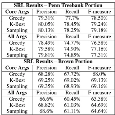
For the past two years CoNLL has had shared tasks on SRL (Carreras and M`arquez (2004) and Carreras and M`arquez (2005)). We used the CoNLL 2005 data and evaluation script. When evaluating semantic role labeling results, it is com-mon to present numbers on both the core argu-ments (i.e., excluding the modifying arguargu-ments) and all arguments. We follow this convention and present both sets of numbers. We give precision,
5
They report their results on the first PASCAL dataset, and use only the development set from the first challenge for learning weights. When we test on the data from the second challenge, we use all data from the first challenge and the development data from the second challenge to learn these weights.
SRL Results – Penn Treebank Portion Core Args Precision Recall F-measure
Greedy 79.31% 77.7% 78.50%
K-Best 80.05% 78.45% 79.24%
Sampling 80.13% 78.25% 79.18% All Args Precision Recall F-measure
Greedy 78.49% 74.77% 76.58%
K-Best 79.58% 74.90% 77.16%
Sampling 79.81% 74.85% 77.31% SRL Results – Brown Portion Core Args Precision Recall F-measure
Greedy 68.28% 67.72% 68.0%
K-Best 69.25% 69.02% 69.13%
Sampling 69.35% 68.93% 69.16% All Args Precision Recall F-measure
Greedy 66.6% 60.45% 63.38%
K-Best 68.82% 61.03% 64.69%
[image:7.595.321.510.61.249.2]Sampling 68.6% 61.11% 64.64% Table 1: Results for semantic role labeling task. The sampled numbers are averaged over several runs, as discussed.
recall and F-measure, which are based on the num-ber of arguments correctly identified. For an argu-ment to be correct both the span and the classifica-tion must be correct; there is no partial credit.
To generate sampled parses, we used the Stan-ford parser (Klein and Manning, 2003). The CoNLL data comes with parses from Charniak’s parser (Charniak, 2000), so we had to re-parse the data and retrain the SRL system on these new parses, resulting in a lower baseline than previ-ously presented work. We choose to use Stan-ford’s parser because of the ease with which we could modify it to generate samples. Unfortu-nately, its performance is slightly below that of the other parsers.
RTE Results
Accuracy Average Precision
Greedy 59.13% 59.91%
[image:8.595.94.269.63.107.2]Sampling 60.88% 61.99%
Table 2: Results for recognizing textual entailment. The sam-pled numbers are averaged over several runs, as discussed.
ran the pipeline using a50-best list, and found the two results to be comparable.
6.2 Textual Entailment
For the second PASCAL RTE challenge, two dif-ferent types of performance measures were used to evaluate labels and confidence of the labels for the text-hypothesis pairs. The first measure is ac-curacy – the percentage of correct judgments. The second measure is average precision. Responses are sorted based on entailment confidence and then average precision is calculated by the following equation:
1
R
n X
i=1
E(i)# correct up to pairi
i (5)
wherenis the size of the test set,Ris the number of positive (entailed) examples, E(i) is an indi-cator function whose value is 1 if the ith pair is entailed, and theis are sorted based on the entail-ment confidence. The intention of this measure is to evaluate how well calibrated a system is. Sys-tems which are more confident in their correct an-swers and less confident in their incorrect anan-swers will perform better on this measure.
Our results are presented in Table 2. We gen-erated 25 samples for each run, and repeated the process 7 times, averaging over runs. Accuracy was improved by 1.5% and average precision by 2%. It does not come as a surprise that the average precision improvement was larger than the accu-racy improvement, because our model explicitly estimates its own degree of confidence by estimat-ing the posterior probability of the class label.
7 Conclusions and Future Work
We have presented a method for handling lan-guage processing pipelines in which later stages of processing are conditioned on the results of earlier stages. Currently, common practice is to take the best labeling at each point in a linguistic analysis pipeline, but this method ignores informa-tion about alternate labelings and their likelihoods. Our approach uses all of the information available,
and has the added advantage of being extremely simple to implement. By modifying your subtasks to generate samples instead of the most likely la-beling, our method can be used with very little ad-ditional overhead. And, as we have shown, such modifications are usually simple to make; further, with only a “small” (polynomial) number of sam-ples k, under mild assumptions the classification error obtained by the sampling approximation ap-proaches that of exact inference. (Ng and Jordan, 2001) In contrast, an algorithm that keeps track only of the k-best list enjoys no such theoretical guarantee, and can require an exponentially large value forkto approach comparable error. We also note that in practice, k-best lists are often more complicated to implement and more computation-ally expensive (e.g. the complexity of generat-ing k sample parses or CRF outputs is substan-tially lower than that of generating thekbest parse derivations or CRF outputs).
The major contribution of this work is not specific to semantic role labeling or recognizing textual entailment. We are proposing a general method to deal with all multi-stage algorithms. It is common to build systems using many different software packages, often from other groups, and to string together the1-best outputs. If, instead, all NLP researchers wrote packages which can gen-erate samples from the posterior, then the entire NLP community could use this method as easily as they can use the greedy methods that are com-mon today, and which do not perform as well.
8 Acknowledgements
We would like to thank our anonymous review-ers for their comments and suggestions. We would also like to thank Kristina Toutanova, Aria Haghighi and the Stanford RTE group for their as-sistance in understanding and using their code.
This paper is based on work funded in part by a Stanford School of Engineering fellowship and in part by the Defense Advanced Research Projects Agency through IBM. The content does not nec-essarily reflect the views of the U.S. Government, and no official endorsement should be inferred.
References
Rens Bod. 1995. The problem of computing the most proba-ble tree in data-oriented parsing and stochastic tree gram-mars. In Proceedings of EACL 1995.
Xavier Carreras and Llu´ıs M`arquez. 2004. Introduction to the CoNLL-2004 shared task: Semantic role labeling. In
Proceedings of CoNLL 2004.
Xavier Carreras and Llu´ıs M`arquez. 2005. Introduction to the CoNLL-2005 shared task: Semantic role labeling. In
Proceedings of CoNLL 2005.
Eugene Charniak. 2000. A maximum-entropy-inspired parser. In Proceedings of the 14th National Conference
on Artificial Intelligence.
Robert G. Cowell, A. Philip Dawid, Steffen L. Lauritzen, and David J. Spiegelhalter. 2003. Probabilistic Networks and
Expert Systems. Springer.
Richard Crouch. 2005. Packed rewriting for mapping se-mantics to KR. In Proceedings of the 6th International
Workshop on Computational Semantics.
Ido Dagan, Oren Glickman, and Bernardo Magnini. 2005. The PASCAL recognizing textual entailment challenge. In
Proceedings of the PASCAL Challenges Workshop on Rec-ognizing Textual Entailment.
Stuart Geman and Mark Johnson. 2002. Dynamic program-ming for parsing and estimation of stochastic unification-based grammars. In Proceedings of ACL 2002.
Joshua Goodman. 1998. Parsing Inside-Out. Ph.D. thesis, Harvard University.
Aria Haghighi, Kristina Toutanova, and Christopher D. Man-ning. 2005. A joint model for semantic role labeling. In
Proceedings of CoNLL 2005.
Liang Huang and David Chiang. 2005. Betterk-best pars-ing. In Proceedings of the 9th International Workshop on
Parsing Technologies.
Lauri Karttunen. 2000. Applications of finite-state trans-ducers in natural-language processing. In Proceesings of
the Fifth International Conference on Implementation and Application of Automata.
Dan Klein and Christopher D. Manning. 2003. Accurate unlexicalized parsing. In Proceedings of ACL 2003. Peter Koomen, Vasin Punyakanok, Dan Roth, and Wen tau
Yih. 2005. Generalized inference with multiple semantic role labeling systems. In Proceedings of CoNLL 2005, pages 181–184.
John Lafferty, Andrew McCallum, and Fernando Pereira. 2001. Conditional Random Fields: Probabilistic models for segmenting and labeling sequence data. In
Proceed-ings of the Eighteenth International Conference on Ma-chine Learning, pages 282–289.
Bill MacCartney, Trond Grenager, Marie de Marneffe, Daniel Cer, and Christopher D. Manning. 2006. Learning to rec-ognize features of valid textual entailments. In
Proceed-ings of NAACL-HTL 2006.
Christopher D. Manning and Hinrich Sch¨utze. 1999.
Foun-dations of Statistical Natural Language Processing. The
MIT Press, Cambridge, Massachusetts.
John T. Maxwell, III and Ronald M. Kaplan. 1995. A method for disjunctive constraint satisfaction. In Mary Dalrymple, Ronald M. Kaplan, John T. Maxwell III, and Annie Zae-nen, editors, Formal Issues in Lexical-Functional
Gram-mar, number 47 in CSLI Lecture Notes Series, chapter 14,
pages 381–481. CSLI Publications.
Andrew Ng and Michael Jordan. 2001. Convergence rates of the voting Gibbs classifier, with application to Bayesian feature selection. In Proceedings of the Eighteenth
Inter-national Conference on Machine Learning.
Charles Sutton and Andrew McCallum. 2005. Joint pars-ing and semantic role labelpars-ing. In Proceedpars-ings of CoNLL
2005, pages 225–228.
Kristina Toutanova, Aria Haghighi, and Christopher D. Man-ning. 2005. Joint learning improves semantic role label-ing. In Proceedings of ACL 2005.
Kristina Toutanova. 2005. Effective statistical models for
syn-tactic and semantic disambiguation. Ph.D. thesis,
Stan-ford University.
Ben Wellner, Andrew McCallum, Fuchun Peng, and Michael Hay. 2004. An integrated, conditional model of informa-tion extracinforma-tion and coreference with applicainforma-tion to citainforma-tion matching. In Proceedings of the 20th Annual Conference