Abstract—In Egypt, there has been a major effort to improve the water supply and also sanitation services although there are still major deficits in rural areas. Remaining a major challenge on the national level, rural drinking water supply is projected to become increasing inadequate with population growth. A part of the water supply comes from the Nile system and the other part comes from groundwater sources mainly by using wells. Typical applications of numerical models to field scale problems generally require large grids that can seldom accommodate cells as small as the actual well diameter. Several methods have been used to simulate a more accurate head at the well scale. The three primary methods are local grid refinement, local analytical correction and local numerical correction. However, all these methods have limitations, especially for applications that involve the development of numerical models for large scale hydrogeologic systems with multiple pumping wells.
The paper presents a hierarchical approach for groundwater modeling and especially for predicting head at the well scale. The hierarchical approach enables converting a large, complex problem into a network of hierarchically nested and dynamically coupled models that can be easily solved. The study aimed to demonstrate that the hierarchical modeling approach and provide an accurate representation of head and groundwater velocities in a well field in large scale hydrogeologic systems.
Index Terms—Analytical method, Groundwater modeling, Hierarchical approach, and Numerical model.
I. INTRODUCTION
There are many water related challenges facing Egypt. The most important challenge is Egypt’s expected population growth which tripled during the last 50 years from 19 millions in 1947 to about 65 millions in 2000 and it is expected to be about 95 millions by the year 2025 [1]. Municipal water demand including water supply to major urban and rural villages is estimated as 4.6 BCM per year. A part of that water comes from the Nile system and the other part comes from groundwater sources. Therefore, providing sufficient drinking water of good quality to the growing population and related
Prof. Dr. Mohamed Said Abd El-Wahab is the head of Scientific Computing department, Faculty of Computer and Information Sciences, Ain Shams University.
Prof. Dr. Mohamed Essam Khalifa is the Dean of Faculty of Computer and Information Sciences , Ain Shams University.
Noran Adel Emara is Teacher Assistant in Scientific Computing Department, Faculty of Computer and Information Sciences, Ain Shams University, Cairo, Eqypt.
socio-economic activities is directed to the use the potential of groundwater for municipal water supply [2].
It is usually impractical in groundwater modeling to employ grids that are comparable in size and dimension to a pumping well. However, predicting head in close proximity to a pumping well (well scale) may be important for many groundwater flow modeling applications, especially in complex environments. In groundwater flow modeling, long term drawdown prediction at the well is critical for proper well design [3]. Moreover, it is important to predict drawdown at the well scale where models are used for evaluation of groundwater management, pollution control, and sustainability strategies.
In numerical models, numerous finite discrete cells, that have relatively large spatial dimensions, are used to represent the aquifer system. A point source or sink of water is injected, or extracted over the volume of aquifer represented by the cell that contains the point source or sink [4]. But, the diameter of the well is typically much smaller than the dimensions of the cell. Field scale problems generally cover large geographic areas that require grids having cells with large spatial dimensions and can seldom accommodate cells as small as the actual well diameter. The resulting simulated head are generally not a good approximation of heads or hydraulic gradients in close proximity to the pumping well, or any other source or sink; numerous small cells are needed to simulate the relatively steep hydraulic gradients near a point source or sink accurately. However, regional model derived heads may be correct at nodes located away from the point source or sink [4], [5].
A lot of methods have been adopted in an attempt to improve the accuracy of simulated heads at the well scale. There are three main methods: the first is the local grid refinement [6], [7], local analytical correction [8], [9], [10], and local nested numerical correction [11], [12], [13]. However, all these methods may have severe limitations, especially for applications that involve the development of numerical models for large scale, complex hydrogeologic systems with multiple pumping wells or other sources or sinks. In particular the application of grid refinement techniques to these complex problems, may lead to slow convergence, numerical oscillations, inefficiencies, and solution failure [14]. In addition, the time and computational resources needed to store and process simulation results may be great.
The objectives of this paper are to address the limitations and drawbacks of the traditional methods used to predict heads at the well scale for large complex groundwater systems , and to present an innovative methodology for determining well
A Hierarchical Approach for Groundwater
Modeling
scale heads for such systems. Interactive Ground Water which uses the hierarchical- modeling approach [14], [15], overcomes the difficulties encountered using traditional finite difference methods in calculating well-scale heads. Moreover, it is capable of modeling large complex groundwater systems in a flexible and computationally efficient framework on typical desktop computers.
In the following sections, we review the traditional methods for calculating hydraulic heads at the well scale, and point out the limitations with the assumptions and implementation of these methods. Then, we introduce the hierarchical modeling approach and explain the concept behind this approach. Finally, we present illustrative examples to verify and show the capabilities of the hierarchical modeling method.
II. TRADITIONAL METHODOLOGIES
There are three main methods employed for predicting the hydraulic head in close proximity to a pumping well using regional scale models are: local grid refinement method [6], [7], [16] local analytical correction method [8], [9], [10], and local nested numerical correction method [11], [12], [13].
A. Local Grid Refinement
Local Grid Refinement represents the most commonly used method to predict detailed well dynamics in a numerical model. The relatively large grid cell from a numerical model is subdivided or refined with progressively smaller spatial dimensions in the area of interest (e.g., surrounding of the well node) [6], [7], [16]. This results in a more accurate estimation of hydraulic head or drawdown at the well scale. In this approach, there is one model with the area of grid refinement that is part of the regional model. This often results in a very large number of grid cells.
In using local refinement for simple or small scale problems, the solution is obtained quickly, and consistency between the regional and local area around the wells is maintained. However, for large-scale, regional groundwater models where there may be a significant increase in the number of nodes, the cost of computation increases exponentially intensive. Additionally, for large problems that involve multiple sources and sinks, multiple scaled of interest, transient flow conditions, complex aquifer structure, and strong anisotropy and heterogeneity, the solution process can become problematic. In these cases, the structure of the matrices may be highly “ill-conditioned”, which often leads to lack of convergence or numerical oscillations [14].
B. Local Analytical Correction
An alternative approach to model detailed well dynamics in a regional model is to use Local Analytical Correction within the cell containing the well. For example, the head calculated at the well node using a finite difference method can be thought to represent the head at an effective distance (
r
e) from thewell node. An estimation of the head in the well can be obtained from formulas based on the following steady-state Thiem equation which can be applied to quasi-steady-state conditions when the rate of removal of water from storage near
the pumping well is zero. The head in the well is calculated from the following equation [4].
w e WT j i w
r r T Q h
h ln 2
, (1)
Where
w
h is the head in the well; hi,jis the head computed by
the finite difference model for the well node (i, j);
Q
WT is thetotal pumping or injection rate from the well; T is the transmissivity in the well cell;
r
eis the effective radial distancemeasured from the node at which head is equal to
j i
h , ; and
r
wis the radius of the actual well. The radius
r
eis the effectivewell-block radius. Prickett [8], Peaceman [9] and Trescott [17] provided an equation, which approximates
r
e based ondifferent model grid sizes. Their assumptions in applying this approximation are: Flow to the well is within a square finite-difference cell (well block) and can be described by a steady-state equation with no source term except for the well discharge; The aquifer is isotropic and homogenous in the well block; Only one well, located at the cell center, is in the well bock; The well fully-penetrates the aquifer; Flow to the well is laminar and Well loss is negligible.
The application of the analytical correction method results in a drawdown prediction that is comparable to the exact solution [17]. However, this method suffers from several limiting factors; one of which is that it can’t easily be applied for multiple sources and sinks within the well block. In addition, the corrected drawdown method is not valid for other general cases, such as variable hydraulic conductivity, variable recharge, anisotropic media with specified orientation, partial well penetration, and transient flow or pumping conditions [5].
C. Local Numerical Correction
A more general approach for modeling detailed local well dynamics is through Local Numerical Correction. With this approach, the relatively large finite-difference grid cell from a regional model is subdivided into multiple cells with progressively smaller spatial dimensions [11], [12], [13]. This results in a more accurate estimation of hydraulic head or drawdown at the well scale.
A model covering a relatively large domain and having grids with large spatial dimensions relative to the well scale is often referred to as the “regional model” and a model with the finer grid is called “submodel”. In order to obtain detailed information for the local model, it is necessary to interpolate grid dependent information from the regional model at the finer grid spacing of the local model. The transformation of information from regional model to local model and the selection of the boundary conditions and starting conditions for the local model are the most important issues using this numerical methodology [12], [18], [19].
solved using multiple, smaller-scale local models. This procedure can be implemented successively in a continuous manner until the desired resolution of the well scale is obtained. Once the local model is created, it performs as an independent model. The primary advantage of this approach is that it can reduce a large and complex matrix system into multiple smaller and better-conditioned matrices.
However, the major drawback to implementing the nested models is that the interaction between the parent and local models (of which there can be several) depends on the offline analysis and processing of model modifications or simulation results from the parent model to obtain the boundary and starting conditions for the local model.
III. HIERARCHICAL MODELING APPROACH
The approach presented for predicting head or drawdown at the well scale employs the concept of hierarchical modeling in a unique, general purpose, and object-oriented computational environment. The approach represents a generalization of the nested grid approach and enables modeling of a large complex system as a network of hierarchically nested patch models. With this approach large , very complex problems are reduced into a number of small, less complex problems that are solved individually in a dynamically- coupled and fully-integrated environment [14].
The hierarchical modeling approach overcomes problems encountered when attempting to solve a very large set of complex, ill-conditioned matrices often encountered with Local Grid Refinement. The approach is more advantageous than the traditional, loosely coupled Local Numerical Correction in that the interaction between the regional model and all submodels is seamless, dynamic, and fully-integrated. In other words, regional-model simulation results (e.g., boundary conditions), and any changes to the regional model propagate automatically to all submodels, without the need for offline post-processing of data or simulation results. This transfer of information between the regional model and submodels is accomplished for each time step in near real-time.
The dynamic- integration eliminates the disconnection in a traditional disjointed nested grid approach and makes generalized hierarchical patch dynamics modeling practical. In particular, this paradigm provides an efficient means of routing data between models and also provides visualization controls at each time step for all models during the simulation. This gives the modelers the perception of using a single model that provides high resolution dynamics at the speed that is very similar to that of a low-resolution coarse-grid model. The object oriented implementation enables flexible, interactive creation of hierarchical models. This hierarchical modeling process is an interactive and recursive process by which a modeler can create a hierarchy of submodels that are embedded in a parent model in order to provide greater detail where it is required.
A. Hierarchical Equations
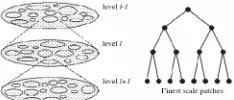
A complex system is represented hierarchically by breaking it “vertically” into many levels and “horizontally” into many patches Fig.(1, left). The dynamics in different patches are
related efficiently to each other through a hierarchical patch network Fig.(1, right). The patches at higher-levels are used to simulate larger-scale dynamics whereas nested patches at lower-levels are used to simulate smaller-scale processes. The upper-level exerts constraints (e.g., as boundary conditions) on the lower-level. The conceptual basis for the hierarchical approach emerges from hierarchy theory [20] and a diversity of studies in various disciplines, including management science, biology, ecology, and system science. The hierarchy theory has been significantly expanded in the context of evolutionary biology and ecology [21].
Fig.(1): Hierarchical decomposition of a groundwater system
Mathematically, the hierarchical approach involves solving a set of hierarchically formulated groundwater equations Table (I) [14]. These equations describe the space-time distribution of
head
h
, velocityu
i, and concentrationc
for a typical patch atlevel
l
defined on l, and its interaction with its ‘‘parent’’ patch onl1 at level1
l , and various ‘‘daughter’’ patches
,...) 2 , 1 ,
(kl1k at level
l
1
Fig.(2).Fig.(2): A typical model patch and its interaction with the parent and daughters.
Table (I) Governing patch dynamics equation Flow
Equations l;
j l l ij i l l s x h K x t h
S
j l l ij l e l i x h K n u
1 (2)
Boundary Conditions j l l ij j l l ij x h K x h K
1 1 or hl hl1 (3)
Initial
Conditions ( ,0) ( ,0)
1 x
h x
hl l (4)
Transport Equations l j l l ij i j l l i l l r x c D x x c u t c
R
(5)
Boundary Conditions i j l l ij i l l i i j l l ij i l l i n x c D n c u n x c D n c u
1 1 1 1 or
1
l
l c
c (6) Initial
Conditions ( ,0) ( ,0)
1
x c x
cil il (7)
Equations (3), (4) and (6) and (7) provides patch boundary and initial conditions, reflecting the coupling with the parent at
level
l
1
. The symbolsn
e, Ss, R; Kijand Dijare effective [image:3.612.385.502.188.238.2] [image:3.612.392.496.368.419.2] [image:3.612.307.563.448.674.2]conductivity-tensor, and dispersion-tensor, respectively;
andr
are the water and solute source/sink term, respectively. It is assumed that groundwater is incompressible, homogeneous, and isothermal and the medium saturated and non-deformable.The equations in Table (I) can be solved sequentially for
,..., 2 , 1 , 0
l based on a scale-dependent discretization through
a systematic process called ‘‘downscaling’’. This process begins with modeling at the highest level on a coarsest grid/time-step and proceeds downward to finer-scales with increasing space-time resolutions. Successive solution of (2) down the hierarchy provides an approximation of the system dynamics and a mechanism to pass field information from high to low levels.
B. Patch Boundary Identification
The hierarchical approach a generalization of the frequently used local numerical correction technique [11] and the marriage of hierarchical modeling and patch dynamics [21] to specifically address the infamous ‘‘curse-of-dimensionality’’ and the associated computational bottlenecks in multi-scale modeling. The way to specify patch boundaries is essentially the same as that in a basic nested approach. In other words, patch boundaries are identified empirically based on the parent-solution behavior, system characteristics, and data densities. Modeling patches are created in localized areas exhibiting much more rapidly-varying dynamics. The patch boundaries are selected such that they are located outside the ‘‘hot-spots’’ or in areas where the parent head varies relatively slowly and is deemed accurate.
In general, identifying patches for local grid refinement may have to be iterative. A patch solution is deemed accurate if it becomes insensitive to changes in the patch boundary location. One may also potentially avoid the need to iterate or minimize the number of trial runs needed if modeling patches are defined ‘‘conservatively’’ or made larger than needed.
IV. STUDY AREA
A small village in Giza Governorate has been selected as an application of the proposed management model of potable water feeding system until year 2040. The village is located in south Giza with temperature ranged between 14o to 28o with rare rain around the year. The village is characterized by medium average of humidity; it ranges between 69% in November to 46% in May. This is due to the scarcity of water surfaces, arable areas, geographical and typographical site. Generally, the region is characterized by moderate winds, the monthly average of wind speed reaches its highest value within March, April, May, and its lowest one in Autumn, regarding that most winds come from the North, North-East and North-West.
The village consists of a group of nomad houses randomly away from each other. There are no paved roads; the only paved one has a rocky nature, extending to the middle of the village. In general, the soil consists of sand, stones and rocks. There are no works concerning water at present, the village depends on daily supply of a tank with the capacity of 5 m3 from a nearby village. The village is fed from a main potable water station by year 2025. The village is in need of a design of available source of
water till year 2025 and a network pipe system to fulfill the requirements of the village and the nearby one [22].
According to 1996 census, the population of the village was 17750 persons. The source of water supply is designed to fulfill the requirements until 2025 while the network is designed until 2040. The village under study is planed to be fed of water from potable pump station by year 2025`which will replace the current wells.
The population increase is calculated by the Geometrical method: Pf = Pp* (1 + A)n, where: Pf is the future census
(person), Pp is the present census (person), A is the annual
percent increasing rate for population and n is the target period for the study. By assuming the rate of population increase 2.0% according to increasing rate of the government, the population is estimated 31521 persons by year 2025.
According to the Egyptian code, the rate for potable water for small villages is 125 liter/capita/day. The increasing rate for per capita is calculated according to the Egyptian Code (2000): Per capita increasing rate = ( (1 + I)n- 1 ) * 100, where: I is the increasing rate for annual consumption (0.1 * percentage of population increasing rate), and n is the number of years. The annual consumption for year 2025 is estimated by 131 liter/capita/day (Average daily consumption. According to the code, maximum monthly rate is estimated by 5776 m3/day (1.2 to 1.6 * Average daily consumption). Assuming that the pumps works 16 hour, the amount of water to be lifted is estimated 361 m3/hr.
Maximum hour rate, according to the code, is 2.5 * Average daily consumption (10312.5 m3/day). Therefore, five wells (with one well capacity of the 100 m3/hr) are needed (four working wells and one standby) to produce minimum 8663 m3/hr. The network pipeline system can be designed to distribute water with minimum discharge of 10312.5 m3/hr [22]. Choosing the number of wells to ensure feeding of the village with water till the target year and choosing the best appropriate scenario for working the wells is covered in [22]. The main concern here is to apply the hierarchical modeling approach to simulate the detailed flow dynamics around the proposed wells.
V. ILLUSTRATIVE APPLICATION
Fig.(3) Layout of the well area
Another difficulty in modeling a well field is representing the exact location of the individual pumping wells, especially those in close proximity to each other. With a regional model, or coarse grid submodel, clusters of closely spaced wells are grouped together in a single well node. A locally refined grid is needed to simulate the impact of individual wells on heads and flow rates.
The distribution of the pumping wells is shown in Fig.(3). The available area of wells, pumps, elevated tank, small workshop, and administrative building is rectangle in shape with length of 45.0 meters and width of 35.0 meters. The area is surrounded by a drain, a road and agricultural areas. The regional model domain is 1000 m by 1000 m with a uniform grid of 100 meters.
The outer boundaries are represented by no-flow boundaries. The no-flow boundaries in the regional model have been placed at this distance so they don’t affect the simulated drawdown in the well field, satisfying the assumption of an infinite aquifer. The aquifer parameters are
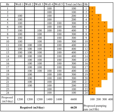
Table (II) wells schedule and total discharge each hour
Fig.(4): Hierarchical modeling network illustrating the relationship between submodels and their parent model for single well (well 4)
as follows: the aquifer depth is 102 m ; the storage coefficient of the aquifer is 0.00005 ; the permeability in the horizontal direction is 2.7 m/day ; the permeability in the vertical direction is 0.2 m/day ; the well radius is 0.1 meter; the pumping rate for each well is 100 m3/hr and the duration of pumping is 24 hours.
Table (II) presents the most appropriate scenarios, which satisfy most of the requirements of having four pumps working 16 hours a day or five wells working 12.8 hour/day. The table shows the time schedule for each well, each column presents the start and end time for each well. The last column sums up the discharge of the wells working at the same time. The figure in right side shows the schedule of wells and the corresponding total discharge. The design of the wells schedule based on minimizing the number of working hours for the wells next to the drain and avoiding the interaction between wells which in turn will reduce the drawdown. In the peak hours (11:00 am to 2:00 pm, 7:00 am to 6:00 pm), four wells are working to satisfy the water requirement in the peak hour [22].
In this section we illustrate the hierarchical modeling approach for modeling near well dynamics through different scenarios in Table (II). The first scenario considers a simple situation involving unsteady flow toward a single well (well 4). The second scenario considers when two pumping wells working at the same time (well 1 and well 4). The third scenario considers when three pumping wells working together (well 1, well 2 and well 4) and the last scenario when the four wells working at the same time (well 1, well2, well 4, well 5). There is no need for the five wells to work in the same time since the average discharged needed as computed before was 361 m3/hr. As each well produces 100 m3/hr, four working wells are enough while the elevated tank can substitute the difference in the maximum hour demand.
Fig.(4) presents the hierarchical-network and solutions to the single well example. The regional model and the six submodels have grid resolutions of 100 m, 50 m, 25 m, 12.5 m, 6.25 m, and 3.125 respectively.
Each model has a grid that is 21 rows by 21 columns in size. It is important to point out that the results from each submodel were obtained and visualized instantaneously. And, with hierarchical modeling, different drawdown values may be Hr Well 1 Well 2 Well 3 Well 4 Well 5 Total (m3/hr) Hr
1 100 100 1 *
2 100 100 2 *
3 100 100 200 3 * *
4 100 100 200 4 * *
5 100 100 100 300 5 * * *
6 100 100 100 300 6 * * *
7 100 100 100 100 400 7 * * * *
8 100 100 100 300 8 * * *
9 100 100 100 300 9 * * *
10 100 100 100 300 10 * * *
11 100 100 100 100 400 11 * * * *
12 100 100 100 100 400 12 * * * *
13 100 100 100 100 400 13 * * * *
14 100 100 100 100 400 14 * * * *
15 100 100 100 300 15 * * *
16 100 100 100 300 16 * * *
17 100 100 100 300 17 * * *
18 100 100 100 100 400 18 * * * *
19 100 100 100 300 19 * * *
20 100 100 100 300 20 * * *
21 100 100 200 21 * *
22 100 100 200 22 * *
23 100 100 23 *
24 100 100 24 *
Proposed
(m3/day) 1200 1200 1200 1400 1600 6600 100 200 300 400
Required (m3/day) Proposed pumping
rate (m3/Hr)
[image:5.612.318.533.50.208.2] [image:5.612.71.285.53.224.2] [image:5.612.61.292.505.730.2]Fig.(5): Hierarchical modeling network illustrating the relationship between submodels and their parent model for two pumping wells (well 1 and well 4)
recomputed, displayed, and analyzed very quickly whenever the model stresses or other model parameters are changed.
Fig.(5) shows the application of hierarchical modeling for two pumping wells. In this example, different levels of sub models are developed for each pumping well. Starting from a coarse model we can successively approach the area of interest and obtain detailed information as close as the effective well radius. The diagram shown in the upper right quadrant of Fig.(5) illustrates the hierarchical relationship between parent models and subsequent models. The remainder of the figure shows the different model domains, pumping wells and simulated drawdown. An examination of the hierarchical tree and the different model domains should be sufficient to understand the relationship between models. The grid resolution from the regional model to finest well-scale model varies between 100 m to 3.125 m.
Fig.(6) shows the application of hierarchical modeling for three pumping wells. In this example, 6 levels with 10 patches are developed. The diagram shown in the upper right quadrant of Fig.(6) illustrates the hierarchical relationship between parent models and subsequent models. In the label of the
submodel a
bc
M ; a represents the generalization level
Fig.(6): Hierarchical modeling network illustrating the relationship between submodels and their parent model for three pumping wells (well 1, well 4 and
well 5)
Fig.(7): Hierarchical modeling network illustrating the relationship between submodels and their parent model for three wells (well 1, well 3, well 4 and well
5)
(grandparent); b represent the parent index and c represent the child index which is referred to the parent index. The remainder of the figure shows the different model domains, pumping wells and simulated drawdown. The grid resolution from the regional model to finest well-scale model varies between 100 m to 3.125 m.
Finally, Fig.(7) shows the hierarchical model approach application to four pumping wells. We model the system incrementally, visualize the results on-the-fly, and ‘‘zoom’’ into subareas when and where we feel there is a need to. We begin with modeling the entire area using a coarse-grid and then make localized-corrections by adding patches or patches-in-a-patch where the solution is judged to be inaccurate. The patch boundaries are interactively located where the parent dynamics are deemed to be adequately resolved. This process is often iterative and one must use judgment to determine the needed patch extent/resolution based on the parent-solution behavior and local system characteristics. Since the entire model-hierarchy is dynamically-coupled, one can readily evaluate how different patch refinement schemes affect the ultimate solutions.
For this example, 16 patches in 7 levels are created, zooming into 4 focused-areas. In general, the number of levels and patches needed to achieve desired resolutions depends on what the modeling objectives are, how complex the problem is, and how powerful the computer is. Obviously, the number of levels required decreases with decreasing problem size and increasing computer power.
VI. SUMMARY AND CONCLUSIONS
local grid refinement method has limiting assumptions that cannot be applied for general groundwater modeling. With numerical methods, Local Analytical Correction creates computational difficulties because of the large number of nodes, and Local Numerical Correction suffers from the discontinuity between parent and submodels and the time and effort required to process data between parent and submodels.
In this paper, an innovative methodology is presented to predict the head at the radius of a pumping well for large scale and complex groundwater flow system. This method employs
the dynamically integrated, object-oriented,
hierarchical-modeling concept resulting in a highly efficient and flexible way to simulate heads at the well scale. When modeling large-scale complex groundwater systems, the Interactive Groundwater hierarchical modeling approach allows the modeler to obtain an accurate solution at the desired grid resolution quickly and with little difficulty. Convergence to a solution using this method is computationally efficient and can be obtained using typical desktop computers, even for large field applications.
ACKNOWLEDGMENT
First, the greatest thankful is to God who provides us with strength and sensibility to keep on going. Second, I would like to thank Prof. Dr. Mohamed Essam Khalifa, the dean of Faculty of Computer and Information Sciences and Prof. Dr Mohamed Said Abdel Wahab, the head of Scientific Computing Department for their supervision, valuable suggestions and encouragement during my study. Third, I wish to express my great gratitude to Dr. Essam Khalifa , Researcher in Ministry of Water Resources and Irrigation for his their valuable discussions and for providing me with the data and application used . Also, I would like to thank Dr. Hatem, Researcher in Ministry of Water Resources and Irrigation for his guidance, help and cooperation.
REFERENCES
[1] CAPMAS, 2000. Statistical Year Books.
[2] Hefny, K., 1998. "Water use in Egypt. Report submitted to the National Water Quality and Availability Management project (NAWQAM)", El-Qanatir, Egypt.
[3] Beljin, M. S. 1987. "Representation of individual wells in two dimensional groundwater modeling". NWWA/IGMC Conference “Solving Groundwater Problems with Models”, February 10-12, at Denver, Clorado.
[4] Anderson, M. P. and W. W. Woessner. 1992. "Applied groundwater modeling: simulation of flow and advection transport," SaDiego: Academic Press.
[5] S. Afshari, R. Mandle, Q. Liu and S. G. 2006. "A Hierarchical Patch Dynamic Approach for Large Complex Groundwater Systems," Groundwater and Application.
[6] Fung, L.S.-K, “An Analysis of the Control-Volume Finite-Element Method for Flexible-Grid Reservoir Simulation,” paper presented at the 1992 IBM Europe Summer Inst. Computational Methods and Tools in Reservoir Modeling, Oberlech, Aug. 17-21.
[7] Gable, C.W., H.E. Trease, and T.A. Cherry, "Geological Applications of Automatic Grid Generation Tools for Finite Elements Applied to Porous Flow Modeling," Proceedings of the 5th International Conference on
Numerical Grid Generation in Computational Fluid Dynamics and Related Fields, Mississippi State University, April 1966, edited by B. Soni, J. Thompson, P. Eiseman and J. Hauser, ERC-MSU Press, 1996. [8] Prickett, T. A. 1967. "Designing pumped well characteristics into
electrical analog models," Ground Water 5 (4): 38 - 46.
[9] Peaceman, D. W. 1978. "Interpretation of Well-Block Pressures in Numerical Reservoir Simulation," Society of Petroleum Engineers Journal 18 (3): 183-194.
[10] Pritchect, J. W., and S. K. Grag. 1980. "Determination of Effective Well Block Radii for Numerical Reservoir Simulations," Water Resources Research 16 (4): 665-674.
[11] Mehl, S., and M. C. Hill. 2002. "Development and evaluation of a local grid refinement method for a block centered finite difference groundwater models using shared nodes," Advances in Water Resources 25 (5):497-511.
[12] Ward, D. S., D. R. Buss, J. W. Mercer, and S. S. Hughes. 1987. "Evaluation of Groundwater Corrective Action at the Chem-Dyne Hazardous-Waste Site Using a Telescopic Mesh Refinement Modeling Approach," Water Resources Research 23 (4): 603-617.
[13] Efendiev, Y.R., Durlofsky, L.J., and Lee, S.H.: “Modeling of subgrid effects in coarse scale simulations of transport in heterogeneous porous media,” Water Resources Research (2000) 36.
[14] Li, S. G., Q. Liu , and S. Afshari. (in review). "Modeling Complex Groundwater Systems Across Multiple Scales – A Hierarchical Computational Steering Environment," Groundwater and Application. [15] Li, S. G. and Q. Liu. 2003." Interactive Groundwater: An Innovative
Digital Laboratory For Groundwater Education and Resear," Computer Applications in Engineering Education.
[16] Heinemann, Z.E., G. Gerken, and G. von Hantelmann, “Using Local Grid refinement in a Multiple-Application Reservoir Simulator,” paper SPE 12255 presented at the 1983 SPE Reservoir Simulation Symposium, San Francisco, Nov. 15-18.
[17] Trescott, P. C., G. F. Pinder, and S. P. Larson. 1976. "Finite-difference model for aquifer simulation in two dimensional with results of numerical experiment," U.S. Geological Survey, Chap. Cl, BK.6.
[18] Townley, L. R. and J. L. Wilson. 1980. "Description of and users’s manual for a finite-element aquifer flow model AQUIFEM-1.," Cambridge Massachusetts: Ralph M. Parson Laboratory Technology Adaption Program.
[19] Buxton, H. and T. E. Reilly. 1986. "A technique for analysis of ground-water systems of regional and subregional scales applied to Long Island," U.S. Geological Survey.
[20] Simon, H. A., 1973. "The organization of complex systems," In: Pattee, Om H. H. (Ed.), Hierarchy Theory: The Challenge of Complex Systems. G. Braziller, New York, pp. 1-27.
[21] Wu, J., David, J., 2002. "A spatially-explicit hierarchical approach to modeling complex ecological systems: theory and applications," Ecological Modeling 153, 7-26.