A New Method for Structure Detection of
Nonlinear ARX model:
ANOVA_BSD
E. Radmaneshfar, M. Karrari
Abstract—Identification of nonlinear dynamic black box models involves structure detection of nonlinear system (i.e. selecting the regressors that have the most contribution to the output and the regressor function) and finally estimation of model parameters. As the NARX representation can describe many nonlinear dynamic models, it will be used here as the desired structure. It should be noted that when the order of the system increases, even for moderately complex systems the number of candidate terms becomes very large. So, structure detection is necessary in order to have an efficient description of the dynamic systems. In this paper, a new method for selecting regressors with the most contribution to the output and finding an efficient representation of nonlinear dynamic systems is presented. The purposed method, named ANOVA_BSD, is based on the combination of analysis of variance and suboptimal bootstrap algorithm. The anticipated structure takes the advantage of nonlinear ARX polynomial to model different nonlinearities of the system, such as sine and cosine functions. The proposed method is tested on two different systems and simulation results show that ANOVA_BSD effectively reduces model complexity without any noticeable loss in the accuracy.
Index Terms— Analysis of variance, Bootstrap, Nonlinear ARX, Regressor, Structure detection.
I. INTRODUCTION
System identification is the problem of building mathematical models of dynamic systems, that is, systems whose outputs depend not only on the current input, but also on the past input and past output values [6]. Assume that the relationship between the output and input is described by NARX model that is initially introduced in [5]. Identifying a NARX model requires structure detection and parameter estimation; structure detection can be divided into two tasks: model order decision and regressors selection (selection of regressors to be included in the model). NARX representation of many nonlinear systems requires only a few terms (i.e. from past values). However, as the order of the system increases, the number of candidate terms becomes very large [1].
Manuscript received December 30, 2005.
E. Radmaneshfar and M. Karrari are with the Department of Electrical Engineering, Amirkabir University of Technology, Tehran, Iran. (E-mail: [email protected], [email protected]
There are different kinds of method for selecting the best subset of regressors that have the most contribution to the output of nonlinear system, i.e. structure detection of nonlinear systems; such as ANOVA [1], stepwise regression [3], LASSO [3], Bootstrap [4] and so on. Each of these methods has their own limitation and may fail when the nonlinearity of the system is complex or when the number of regressors is too large.
In this paper, the analysis of variance (ANOVA) [3] and suboptimal bootstrap structure detection algorithm (BSD) [4], are combined for selecting the significant terms of NARX model for somehow complex nonlinear system. Also recursive least squares (RLS) is used for parameter estimation of remaining regressors. The input/output data used for identification, selection of the significant regressors and also model validation is obtained from the simulated model.
The main idea of ANOVA is comparing the variances of different combinations of candidate regressors and conclude about which ones actually contributes to the output [1].
Suboptimal Bootstrap algorithm is based on resampling technique for obtaining a new data set instead of repeating the experiments [7]. With bootstrap technique, observations are randomly reassigned, and then estimates are recomputed. These assignments and recomputations are done a large number of times and treated as repeated experiments. In the context of structure detection, bootstrap method is used in this paper to detect spurious parameters of the over-parameterized model; i.e. those parameters whose estimated values cannot be distinguished from zero.
The NARX representation can be found in section II. Structure detection technique, ANOVA is described in section III. Suboptimal bootstrap structure detection algorithm is discussed in section IV and the proposed method (ANOVA_BSD algorithm) is presented in section V. Computer simulation results of applying the ANOVA_BSD on a simulated nonlinear model are presented in section VI and finally conclusions are drawn in section VII.
II. THE NARX MODEL
The NARX model was initially proposed in [5], takes the form of the following nonlinear differential equation:
)) ( ),..., 1 ( ), ( ),..., 1 ( ( )
(t f yt yt ny ut ut nu
y (1)
One of the popular representations for the NARX model in eq. (1) is the polynomial representation, which takes the function f (.) as a polynomial of degree l and gives the form as:
¦ ¦
¦¦
¦
n i i i i n i i i i i n i n i i i i i i i i n i t x t x t x f t x t x f t x f t y l l l 1 ... 1 1 0 1 1 2 1 ) 1 ( 2 1 1 2 12 1 2 1 1 1 1 )) ( ),... ( ), ( ( ... ... )) ( ), ( ( )) ( ( ) (
T
l m t x t x t x t x f k m m m i m k i i i i i i i ii ( (), ( ),... ())
3
( ),1d d1 ... ... 1 2 12 2 1 T (2) Where m i i i12...
T are parameters, n= n u + n y and
°¯ ° ® d d d d 1 )) ( ( 1 ) ( ) ( u y y y y k n n k n n k t u n k k t y t x (3) Degree of the multivariable polynomial is defined as the highest order among all terms.
Since NARX representation is linear in its parameters, linear regression can be used for parameter estimation in structure detection.
Identifying a NARX model requires two steps: 1. Parameter estimation
2. Structure detection that can be divided into: a. Model order selection
b. Selecting which parameters to be included in the model
Model order selection is considered as a part of structure detection. Determination of the model order restricts the choice of terms to be considered.
For NARX models, the system order may be defined as
@
l n nO{[ u y (4)
The maximum number of terms in a NARX model with n u and n y dynamic terms and l the order nonlinearity is [4]:
1 , ) 1 ( 0 1 1
¦
p i i n n p p p p u y i i l i i (5)As a result, the number of candidate terms becomes very large for even moderately complex models, making structure detection difficult. Defining the maximum number of terms, p, as the number of candidate terms to be initially considered for identification, parameter estimation involves determining values of these parameters.
NARX representation of many nonlinear systems requires only a few terms. However, as the order of the system increases, the number of candidate terms becomes very large (5). To put it in a nutshell, the structure detection task is to find a subset of candidate terms that describes the system output best. Analysis of variance
A. A simple idea
Suppose u is periodic and y depends only on u(t-T). Then every time that u(t-T) has the same value as one period before,
y(t)should also have the same value as one period before, apart from the noise term e(t). In other words, the variance of y(t) calculated for these values of t (call it V1) should be the variance of e(t). The variance of e(t)is typically unknown. However, if we check the times t when the pair
>
u(tT) u(t2T)@
has the same value, the variance of y(t)for these t should also be aroundV1, If y(t) does not depend on u(t-2T). By comparing the variances for different combinations of candidate regressors we could thus draw conclusions about which ones y(t)actually depends on [1]
B. ANOVA
The statistical analysis method ANOVA [3] is a widely spread tool for finding out which factors contribute to given measurements. The method is based on the hypothesis tests with F-distributed test variables computed from the residual quadratic sum. Here the fixed effects model with two factors will be described:
ijk ij j i ijk
y PW E (WE) H (6)
Assume that the collected measurement data can be described by a linear statistical model where the ijk’s are independent Gaussian distributed random variables with zero mean and constant variance 2. The parameter Pis the overall mean. For each (quantized) level i=1,2,…,a of the first regressor 1(t), there is a corresponding effect i and for each level j=1,2,…,b of the second regressor 2(t)the corresponding effect is j. The interaction between the regressors is described by the parameters ()ij.
Since the regressors are quantized, it is a very simple procedure to estimate the model parameters by computing means:
¦
¦¦
¦¦
¦¦¦
n k ijk ij a i n k ijk j b j n k ijk i a i b j n k ijk y n y y an y y bn y y abn y 1 . 1 1 . . 1 1 ..1 1 1
... 1 1 1 1 (7)
E AB B A a
i b
j n
k
ij ijk
j i a
i b
j ij
b
j j a
i i a
i b
j n
k ijk T
SS SS SS SS
y y
y y y y n
y y an y
y bn
y y SS
¦¦¦
¦¦
¦
¦
¦¦¦
1 1 1
2 .
2 ... . . ..
1 1
.
2 ... 1
. . 2
... 1
..
1 1 1
2 ...
) (
) (
) ( ) (
) (
(8)
Each part is related to one batch of parameters. If all the parameters in the batch are zero, the corresponding quadratic sum is 2-distributed if divided by the true variance 2. Since the
true variance is not available, the estimate
) 1 (
2
n ab
SSE
V is
used to form F -distributed test variables, e.g., for i;
)) 1 ( (
) 1 (
n ab SSE
a SS A
A
Q (9)
If all theWi’s are zero, Abelongs to an F -distribution with a-1 and ab(n-1) degrees of freedom. If any i is nonzero, it will give a large value ofQA, compared to an F -table. This is of course, a test of the null hypothesis that all the i’s are zero, which corresponds to the case where the regressor 1 does not have any main effect on the measurementsy.
III. BOOTSTRAP STRUCTURE DETECTION ALGORITHM
A. Bootstrap
Bootstrap techniques have received considerable attention due to the availability of affordable and powerful computers [4]. The bootstrap is a numerical procedure for estimating parameter statistics that requires few assumptions. The conditions needed to apply bootstrap to system identification are quite mild; namely, that the errors be independent identically distributed and have zero-mean. Consequently, we hypothesize that bootstrap might be a useful tool for structure detection of non-linear models.
In system identification it is necessary to form an estimate of unknown parameters of a random process, using a set of sample values. These can be computed using the recursive least square (RLS) estimator. Parameter statistics are also needed to make a probability statement with respect to unknown true parameter values. One probability statement is, to assign two limits to a parameter, and assert that, with some specified probability, the true value of the parameter will be situated between these limits, which constitute the confidence interval.
With bootstrap technique, observations are randomly reassigned, and estimates recomputed. These assignments and recomputations are done a large number of times and treated as repeated experiments. In the context of structure detection, bootstrap method is used in this paper to detect spurious parameters of the over-parameterized model; those parameters whose estimated values cannot be distinguished from zero.
Application of bootstrap to structure detection involves two steps:
First step: computing a series of parameter replications, in which bootstrap data is generated to compute new bootstrap parameter estimates;
Second step: forming percentile intervals for hypothesis testing, where the significance of the parameters is determined. Bootstrap data is formed by first estimating the residuals of the identified model; these residuals are then resampled with replacement, centered and then added to the predicted output to generate bootstrap replications of the output [2]. B bootstrap data sets are generated to estimate B bootstrap parameter replications.
Significance of the parameters is determined by forming percentile intervals. The estimates from B parameter replications are ranked in increasing order and the B th and
B(1-) th values in the ordered list of the B replications are used as an upper and lower bound for the parameter deviation with an th and (1-) th level of significance, respectively [4]. The significance of each parameter is determined by checking if 0 lies in its interval: if so, the parameter is rejected. This leads to the following algorithm for structure detection of linear-in-the-parameter models.
An important drawback in the context of bootstrap though, is that the maximum model order is considered known, that is, the maximum number of lagged inputs, the maximum number of lagged outputs and the maximum order on the polynomial expansion are considered as known.
B. Suboptimal Bootstrap structure detection algorithm Based on what stated in the previous part, BSD algorithm is as follows:
1. Compute an initial estimate of the unknown parameter vector using RLS as: Tˆ (<zuT<zu)1<zuTZ
2. Estimate the residuals as: Hˆ ZZˆ
3. Generate B bootstrap data sets asZˆ <TˆHˆ
4. Compute B bootstrap parameter replications as:
<T < 1< TZ
) (
ˆ T
5. Form percentile intervals for each parameter by ranking estimates from the B parameter replications in increasing order.
6. Estimate the upper and lower bounds of each parameters confidence interval for a desired level of significance. 7. Determine if zero lies in the interval of each parameter in
the vector.
8. If zero lies in the interval for any parameter remove it from the regression.
9. Compute a new estimate of the parameter vector and residuals as in 1& 2.
10. Go to 3 until convergence. IV. ANOVA_BSD A. The problem with BSD algorithm
structure detection using BSD becomes a time consuming process and needs a lot of computation. For example, if we want to determine the significant regressors for the second order system that it is supposed to have 3 lagged inputs and 3 lagged outputs, from (5) initially we must estimate the parameters of the system with 35 candidate regressors, which is too much for even moderately nonlinear systems.
Another problem with BSD algorithm is that it fails to find NARX representation for the structure of complex nonlinear functions such as sine, cosine or when in the real structure of system multiplication happens.
B. The problem with ANOVA
ANOVA just finds the regressors that have contribution on the output without computing the parameters of remaining regressors. In other words, it does not say anything about the
)
(f (1) , thus with applying ANOVA on the data just the contribution of different regressors on the output can be decided, and nothing can be found about the system function and also the value of parameters for remaining regressors. Also, ANOVA does not perform well when real structure of the system has additive function.
C. ANOVA_BSD
From what stated in the previous sections, it seems that combination of ANOVA and BSD will perform better than both of them alone for structure detection of nonlinear systems with complex nonlinear functions such as sine, cosine and so on in their natural structure or have a lot of candidate regressors initially.
When the number of candidate regressors is initially too large, it is reasonable to reduce the number of them before applying the BSD. ANOVA is a good tool for this purpose, but take into consideration that with ANOVA we can just find the contributed regressors on the output, and the structure of the understudied system ( f ) (1) is still unknown. After applying the ANOVA and finding the most contributed regressors we can assume that the understudied system has NARX representation and try to build this representation with the remaining regressors, i.e. finding the related regressors using BSD algorithm with RLS as an identification technique. D. ANOVA_BSD Algorithm
Based on what stated in the previous part, ANOVA_BSD algorithm is as follows:
1) Determine the order of the NARX system (4) from experiment or physical insight to the system.
2) Apply the ANOVA to basic set of candidate regressors, these regressors consist of input, delayed input and also delayed output and their combination to assumed order.
3) With remaining regressors construct the NARX representation.
4) Apply the BSD algorithm to the remained NARX representation of the systems and remove the insignificant regressors of NARX representation and compute the related parameters.
V. SIMULATION
A. First example Consider the system
) ( )) ( cos( * )) ( sin( )
(t ut ut et
y (10)
Where input signal u(t) is as an independent, identically distributed random signal from the uniform distribution, between [-pi/4 pi/4] and it is quantized into four equal intervals for applying ANOVA. The noise e(t) is Gaussian noise with zero mean and constant variance (in this example it is equal to one). The reasonable sampling time is equal to 50 ms.
By applying ANOVA to the assumed model with 2 lagged inputs, and also 2 lagged outputs it was concluded that from 28 candidate regressors only u(t) , u(t-2) and y(t-2) have contribution to the output. The result of applying ANOVA to the assumed system is shown in Fig. 1.
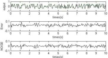
[image:4.612.342.532.420.524.2] [image:4.612.350.532.561.659.2]Now, by assuming the order 3 for NARX representation the BSD algorithm is started. By (5) the assumed NARX representation must have 34 candidate regressors, but by applying ANOVA this number is reduced to 9. By applying BSD it is concluded that with 95% confidence the understudied system can be estimated by y(t)=0.9863u(t)-0.5756u3(t).By knowledge from Taylor series, it is expected to obtain such results. It should be noted that, for model validation 200 data points have been used that have not been used in the training phase. Validation results for the first example are depicted in Fig. 1 and Fig. 2. In the figure the simulated output, true output, and the error (difference between true output and the simulated output) are plotted.
Fig. 1: The result of ANOVA for the first example, it can be seen that the regressors 1,3 and 5 have the most contribution to the output.
Fig. 2: Model validation with 200 data points, the error is the difference between the true output and simulated output.
B. Second example Consider the system
) ( )) 2 ( exp( * )) 1 ( cos( * )) ( sin( )
(t ut u t ut et
Where input signal is as an independent, identically distributed random signal from the uniform distribution, between [-pi/2 pi/2] and it is quantized into four equal intervals for applying ANOVA. The noise e(t) is Gaussian with zero mean and constant variance (in this example it is equal to one). The reasonable sampling time is equal to 50 ms; the other configurations are as before.
) (t u
By applying ANOVA to the assumed model with 2 lagged inputs, and also 2 lagged outputs it is concluded that from 28 interacted regressors only u(t),u(t)*u(t-1),u(t)*u(t-2),u(t)*y(t-2) and u(t-1)*y(t-2) have contribution to the output. The ANOVA results are shown in Fig. 3.
Now, by assuming the order 3 for NARX representation we the BSD algorithm is started. By (5) the assumed NARX representation must have 34 candidate regressors, but by applying ANOVA this number is reduced to 15. By applying BSD it is concluded that with 95% confidence the understudied system can be estimated by:
) 2 ( ) 1 ( 0250 . 0 ) 2 ( ) ( 0273 . 0
) 2 ( ) ( 3169 . 0 ) 2 ( ) ( 6518 . 0 ) 1 ( ) ( 4797 . 0
) 1 ( ) ( 0463 . 0 ) ( 1079 . 0 ) ( 0203 . 1 ) (
2
2 2
2 3
t y t u t
y t u
t u t u t
u t u t
u t u
t u t u t
u t
u t
[image:5.612.54.282.335.451.2]y
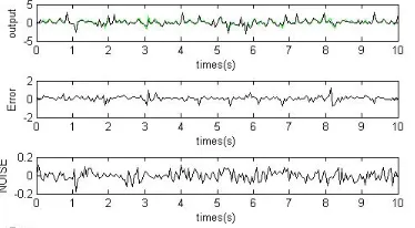
[image:5.612.80.267.489.592.2]Fig. 4 shows the validation results for the second example.
Fig. 3: The result of ANOVA for the second example, it is seen that the regressor 1,6,7,9 and 12 have contribution on the output
Fig. 4: Model validation with 200 data points, the error is the difference between the true output and simulated output.
VI. CONCLUSION
In this paper a new method for structure detection of NARX models was proposed. It is concluded from the computer simulation results that the NOVA_BSD method is a good alternative to BSD for detecting a parsimonious structure, when the understudied model has complex structure. The number of regressor and therefore the complexity of the system are reduced by applying the ANOVA to the nonlinear understudied model. Also, it should be noted that with ANOVA, just the
contributed regressors are found and the system function is still unknown, so by applying BSD to the reduced system and assuming NARX representation the system parsimonious structure can be found.
REFERENCES
[1] Ingela Lind, Lennart Ljung, “Regressor selection with the analysis of variance method”, Automatica, vol. 41,2005, pp. 693 – 700
[2] Sunil l. Kukreja, Henrietta l. Galiana, Robert Kearney, “A bootstrap method for structure detection of NARMAX models”, int. J. Control, vol. 77, no. 2, 132–143 20 January 2004
[3] I. Lind. “Regressor selection in system identification using ANOVA technical Report Licentiate Thesis no 921, Department of Electrical Engineering, Linkoping university, SE-581,Nov. 2001
[4] Sunil L. Kukreja, “A Suboptimal Bootstrap Method for Structure Detection of NARMAX Models”, Report no: LiTH-ISY-R-2452, May 2002
[5] S.A Billings and I.J. Leontaritis, “Parameter estimation techniques for nonlinear system”, in the 6th IFAC symposium on Identification and System Parameter Estimation, Washington DC, , 1982, pp.235-244. [6] Ljung , “System Identification Theory for the User”. Prentice Hall, Inc.,
Englewood Cliffs, New Jersey, second edition, 1999