http://wrap.warwick.ac.uk
Original citation:
Mijatović, Aleksandar, Vidmar, Matija and Jacka, Saul D.. (2015) Markov chain approximations to scale functions of Lévy processes. Stochastic Processes and their Applications, 125 (10). pp. 3932-3957.
Permanent WRAP url:
http://wrap.warwick.ac.uk/75698
Copyright and reuse:
The Warwick Research Archive Portal (WRAP) makes this work by researchers of the University of Warwick available open access under the following conditions. Copyright © and all moral rights to the version of the paper presented here belong to the individual author(s) and/or other copyright owners. To the extent reasonable and practicable the material made available in WRAP has been checked for eligibility before being made available.
Copies of full items can be used for personal research or study, educational, or not-for-profit purposes without prior permission or charge. Provided that the authors, title and full bibliographic details are credited, a hyperlink and/or URL is given for the original metadata page and the content is not changed in any way.
Publisher’s statement:
© 2015, Elsevier. Licensed under the Creative Commons Attribution-NonCommercial-NoDerivatives 4.0 International http://creativecommons.org/licenses/by-nc-nd/4.0/ A note on versions:
The version presented here may differ from the published version or, version of record, if you wish to cite this item you are advised to consult the publisher’s version. Please see the ‘permanent WRAP url’ above for details on accessing the published version and note that access may require a subscription.
PROCESSES
ALEKSANDAR MIJATOVI ´C, MATIJA VIDMAR, AND SAUL JACKA
Abstract. We introduce a general algorithm for the computation of the scale functions of a spectrally negative L´evy processX, based on a natural weak approximation of X via upwards skip-free continuous-time Markov chains with stationary independent increments. The algorithm
consists of evaluating a finite linear recursion with its (nonnegative) coefficients given explicitly in terms of the L´evy triplet of X. Thus it is easy to implement and numerically stable. Our main result establishes sharp rates of convergence of this algorithm providing an explicit link between
the semimartingale characteristics ofX and its scale functions, not unlike the one-dimensional Itˆo diffusion setting, where scale functions are expressed in terms of certain integrals of the coefficients of the governing SDE.
1. Introduction
It is well-known that, for a spectrally negative L´evy processX[5, Chapter VII] [33, Section 9.46], fluctuation theory in terms of the two families of scale functions, (W(q))
q∈[0,∞) and (Z(q))q∈[0,∞),
has been developed [22, Section 8.2]. Of particular importance is the functionW :=W(0), in terms
of which the others may be defined, and which features in the solution of many important problems of applied probability [21, Section 1.2]. It is central to these applications to be able to evaluate scale functions for any spectrally negative L´evy processX.
The goal of the present paper is to define and analyse a very simple novel algorithm for computing
W. Specifically, to compute W(x) for some x >0, choose small h >0 such that x/his an integer. Then the approximationWh(x) toW(x) is given by the recursion:
Wh(y+h) =Wh(0) + y/h+1
X
k=1
Wh(y+h−kh)
γ−kh
γh
, Wh(0) = (γhh)−1 (1.1)
fory= 0, h,2h, . . . , x−h, where the coefficientsγh and (γ−kh)k≥1 are expressible directly in terms
of the L´evy measureλ, (possibly vanishing) Gaussian componentσ2and driftµof the L´evy process
X, as follows. Let:
˜
σh2:= 1 2h2 σ
2 +
Z
[−h/2,0)
y21[−V,0)(y)λ(dy)
!
, µ˜h:= 1
2h µ+h X
k∈N
kλ
−k−1
2
h,
−k+1 2
h
∩[−V,0)
! ,
2010Mathematics Subject Classification. 60G51.
Key words and phrases. Spectrally negative L´evy processes, algorithm for computing scale functions, sharp con-vergence rates, continuous-time Markov chains.
MV acknowledges the support of the Slovene Human Resources Development and Scholarship Fund under contract
number 11010-543/2011. We thank Ron Doney for suggesting one of the examples in this paper.
where V equals 0 or 1 according as to whether λ is finite or infinite, and the drift µ is relative to the cut-off function ˜c(y) := y1[−V,0)(y) (see Eq. 2.1 for the Laplace exponent of X); remark
˜
σ2
h=σ2/2h2 and ˜µh=µ/2h, when V = 0. Then the coefficients in (1.1) are given by:
γh:= ˜σh2+1(0,∞)(σ2)˜µh+1{0}(σ2)2˜µh, γ−h := ˜σ2h−1(0,∞)(σ2)˜µh+λ(−∞,−h/2] (1.2)
γ−kh:=λ(−∞,−kh+h/2], wherek≥2. (1.3)
Indeed, the algorithm just described is based on a purely probabilistic idea of weak approxima-tion: for small positiveh,Xis approximated by what is a random walkXhon a lattice with spacing
h, skip-free to the right, and embedded into continuous time as a compound Poisson process (see Definition 3.1). Then, in recursion (1.1), Wh is the scale function associated to Xh — it plays a probabilistically analogous rˆole for the process Xh, as does W for the process X. Thus W
h is
computed as an approximation to W (see Proposition 3.5).
When it comes to existing methods for the evaluation of W, note that analytically W is char-acterized via its Laplace transform Wc,Wc in turn being a certain rational function of the Laplace
exponent ψ of X. However, already ψ need not be given directly in terms of elementary/special functions, and less often still is it possible to obtain closed-form expressions forW itself. The user is then faced with a Laplace inversion algorithm [13] [21, Chapter 5], which (i) necessarily involves the evaluation ofψ, typically at complex values of its argument and requiring high-precision arithmetic due to numerical instabilities; (ii) says little about the dependence of the scale function on the L´evy triplet ofX (recall thatψdepends on a parametric complex integral of the L´evy measure, making it hard to discern how a perturbation in the L´evy measure influences the values taken by the scale function); and (iii) being a numerical approximation, fails a priori to ensure that the computed values of the scale function are probabilistically meaningful (e.g. given an output of a numerical Laplace inversion, it is not necessary that the formulae for, say, exit probabilities, involving W, should yield values in the interval [0,1]).
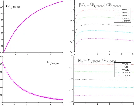
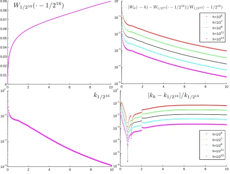
By contrast, it follows from (1.1) and the discussion following, that our proposed algorithm (i) requires no evaluations of the Laplace exponent ofXand is numerically stable, as it operates in nonnegative real arithmetic [31, Theorem 7]; (ii) provides an explicit link between the deterministic semimartingale characteristics ofX, in particular its L´evy measure, and the scale functionW; and (iii) yields probabilistically consistent outputs. Further, the values of Wh are so computed by a simple finite linear recursion and, as a by-product of the evaluation ofWh(x), valuesWh(y) for all the grid-points y= 0, h,2h, . . . , x−h, x, are obtained (see Matlab code for the algorithm in [28]), which is useful in applications (see Section 6 below).
Our main results will (I) show that Wh converges to W pointwise, and uniformly on the grid with spacing h (if bounded away from 0 and +∞), for any spectrally negative L´evy process, and (II) establish sharp rates for this convergence under a mild assumption on the L´evy measure.
Due to the explicit connection between the coefficients appearing in (1.1) and the L´evy triplet of
of the scale function requires numerical evaluation of certain integrals of the coefficients of the SDE driving said diffusion (for the explicit formulae of the integrals see e.g. [9, Chapters 2 and 3]). Indeed, we express W as a single limit, as h ↓ 0, of nonnegative terms explicitly given in terms of the L´evy triplet. This is more direct than the Laplace inversion of a rational transform of the Laplace exponent, and hence may be of purely theoretical significance (e.g. [30, Remark 3.3]).
Finally, note that an algorithm, completely analogous to (1.1), for the computation of the scale functions W(q), and also Z(q), q ≥ 0, follows from our results (see Proposition 3.5, Eq. (3.1)
and (3.2)) and presents no further difficulty for the analysis of convergence (see Theorem 1.2 below). Indeed, our discretization allows naturally to approximate other quantities involving scale functions, which arise in application: the derivatives of W(q) by difference quotients of W(q)
h ; the integrals of a continuous (locally bounded) function against dW(q) by its integrals againstdW(q)
h ; expressions of the form Rx
0 F(y, W
(q)(y))dy, where F is continuous locally bounded, by the sums
Pbx/hc−1
k=0 F(kh, W (q)
h (kh))h etc. (See Section 6 for examples.)
1.1. Overview of main results. The key idea leading to the algorithm in (1.1) is best described by the following two steps: (i) approximate the spectrally negative L´evy processXby a continuous-time Markov chain (CTMC) Xh with state space
Zh :={hk:k∈Z}(h∈(0, h?) for some h?>0), as described in Subsection 2.1; (ii) find an algorithm for computing the scale functions of the chain Xh. The approximation in Subsection 2.1 implies that Xh is a compound Poisson (CP) process, which is not spectrally negative. However, since the corresponding jump chain of Xh is a skip-free to the right Zh-valued random walk, it is possible to introduce (right-continuous, nondecreasing) scale functions (Wh(q))q≥0 and (Zh(q))q≥0 (with measuresdWh(q)and dZh(q)supported
in Zh), in analogy to the spectrally negative case. Moreover, as described in Proposition 3.5, a straightforward recursive algorithm is readily available for evaluating exactly any function in the families (Wh(q))q≥0 and (Zh(q))q≥0 at any point. More precisely, it emerges, that for each x ∈ Zh,
Wh(q)(x) (resp. Zh(q)(x)) obtains as a finite linear combination of the preceding values Wh(q)(y) (resp. Zh(q)(y)) for y ∈ {0, h, . . . , x−h}; with the starting value Wh(q)(0) (resp. Z(q)(0)) being
known explicitly. This is in spite of the fact that the state space of the L´evy process Xh is in fact theinfinite latticeZh.
In order to precisely describe the rates of convergence of the algorithm in (1.1), we introduce some notation. Fixq ≥0 and define for K, G bounded subset of (0,∞):
∆KW(h) := sup x∈Zh∩K
W
(q)
h (x−δ
0h)
−W(q)(x)
and ∆
G
Z(h) := sup x∈Zh∩G
Z
(q)
h (x)−Z
(q)(x) ,
whereδ0 equals 0 ifX has sample paths of finite variation and 1 otherwise. We further introduce:
κ(δ) :=
Z
[−1,−δ)|
y|λ(dy), for any δ≥0.
Assumption 1.1. There exists ∈(1,2)with:
(1) lim supδ↓0δλ(−1,−δ)<∞ and
(2) lim infδ↓0
R
[−δ,0)x
2λ(dx)/δ2−>0.
Note that this is a fairly mild condition, fulfilled if e.g. λ(−1,−δ) “behaves as”δ−, asδ ↓0; for a precise statement see Remark 5.10.
Here is now our main result:
Theorem 1.2. LetKandGbe bounded subsets of(0,∞),K bounded away from zero whenσ2= 0.
If κ(0) =∞, suppose further that Assumption 1.1 is fulfilled. Then the rates of convergence of the
scale functions are summarized by the following table:
λ(R) = 0 ∆KW(h) =O(h2) and ∆GZ(h) =O(h) 0< λ(R) & κ(0)<∞ ∆WK(h) + ∆GZ(h) =O(h)
κ(0) =∞ ∆K
W(h) + ∆GZ(h) =O(h2 −)
Moreover, the rates so established are sharp in the sense that for each of the three entries in the
table above, examples of spectrally negative L´evy processes are constructed for which the rate of
convergence is no better than stipulated.
Remark 1.3. (1) The rates of convergence depend on the behaviour of the tail of the L´evy measure at the origin; by contrast behaviour of Laplace inversion algorithms tends to be susceptible to the degree of smoothness of the scale function (for which see [12]) itself [1].
(2) More exhaustive and at times general statements are to be found in Propositions 5.8, 5.9 and 5.11. In particular, the case σ2>0 andκ(0) =∞does not require Assumption 1.1 to be fulfilled,
although the statement of the convergence rate is more succinct under its proviso. Furthermore, in the interest of space, we present sharpness of the rates for the functions W(q) in the case when
σ2 >0 only. For additional examples in this direction, please see the extended arXiv version [30].
(3) The proof of Theorem 1.2 consists of studying the differences of the integral representations of the scale functions. The integrands decaying only according to some power law makes the analysis much more involved than was the case in [29], where the corresponding decay was exponential. In particular, one cannot, in the pure-jump case, directly apply the integral triangle inequality. The structure of the proof is explained in detail in Subsection 5.1.
(4) Since scale functions often appear in applications (see Section 1.2 below) in the form
W(q)(x)/W(q)(y) (x, y > 0, q ≥ 0), we note that the rates from Theorem 1.2 transfer directly
to such quotients, essentially because Wh(q)(y) → W(q)(y) ∈ (0,∞), as h ↓ 0, and since for all
h∈(0, h?), W(q)1(y) −
1
Wh(q)(y) =
Wh(q)(y)−W(q)(y)
W(q)(y)W(q) h (y)
.
(5) For a result concerning the derivatives ofW(q) see Proposition 5.13.
and [5, Chapter VII], while an excellent account of available numerical methods for computing them can be found in [21, Chapter 5]. Examples, few, but important, of processes when the scale functions can be given analytically, appear e.g. in [17]; and in certain cases it is possible to construct them
indirectly [21, Chapter 4] (i.e. not starting from the basic datum, which we consider here to be the characteristic triplet ofX). Finally, in the special case whenXis a positive drift minus a compound Poisson subordinator, we note that numerical schemes for (finite time) ruin/survival probabilities (expressible in terms of scale functions), based on discrete-time Markov chain approximations of one sort or another, have been proposed in the literature (see [36, 16, 11, 15] and the references therein).
In terms of applications of scale functions in applied probability, there are numerous identities concerning boundary crossing problems and related path decompositions in which scale functions feature [21, p. 100]. They do so either (a) indirectly (usually as Laplace transforms of quantities which are ultimately of interest), or even (b) directly (then typically, but not always, as probabilities in the form of quotientsW(x)/W(y)). For examples of the latter see the two-sided exit problem [5, Chapter VII, Theorem 8]; ruin probabilities [22, p. 217, Eq. (8.15)] and the Gerber-Shiu measure [23, Section 5.4] in the insurance/ruin theory context; laws of suprema of continuous-state branching processes [8, Proposition 3.1]; L´evy measures of limits of continuous-state branching processes with immigration (CBI processes) [20, Eq. (3.7)]; laws of branch lengths in population biology [24, Eq. (7)]; the Shepp-Shiryaev optimal stopping problem (solved for the spectrally negative case in [4, Theorem 2, Eq. (30)]); [26, Proposition 1] for an optimal dividend control problem. A further overview of these and other applications of scale functions (together with their derivatives and the integrals Z(q)), e.g. in queuing theory and fragmentation processes, may be found in [21, Section
1.2], see also the references therein. A suite of identities involving Laplace transforms of quantities pertaining to the reflected process ofX appears in [27].
1.3. Organisation of the remainder of the paper. Section 2 provides the setting, gives some preliminary observations/comments and fixes general notation. Section 3 introduces upwards skip-free L´evy chains (they being the continuous-time analogues of random walks, which are skip-skip-free to the right), describes their scale functions and how to compute them. In Section 4 we demonstrate pointwise convergence of the approximating scale functions to those of the spectrally negative L´evy process. Then Section 5 goes on to study the rate at which this convergence transpires. Finally, Section 6 provides some numerical illustrations and further discusses the computational side of the proposed algorithm.
2. Setting, preliminary observations/comments, and general notation
Throughout this paper we let X be a spectrally negative L´evy process (i.e. X has stationary independent increments, is c`adl`ag, X0 = 0 a.s., the L´evy measure λ of X is concentrated on
ψ(β) := logE[eβX1] (β ∈ {γ ∈
C:<γ ≥0}=:C→), can be expressed as (see e.g. [5, p. 188]):
ψ(β) = 1 2σ
2β2+µβ+Z
(−∞,0)
eβy−β˜c(y)−1λ(dy), β ∈C→. (2.1)
The L´evy triplet of X is thus given by (σ2, λ, µ) ˜
c, ˜c := idR1[−V,0) with V equal to either 0 or 1,
the former only if R
[−1,0)|x|λ(dx) <∞ (where idR is the identity on R). Further, when the L´evy
measure satisfiesR
[−1,0)|x|λ(dx)<∞, we may always expressψin the formψ(β) = 1 2σ
2β2+µ 0β+
R
(−∞,0) e
βy−1
λ(dy) for β ∈ C→. If in addition σ2 = 0, then necessarily the drift µ0 must be
strictly positive,µ0 >0 [22, p. 212].
2.1. The approximation. We now recall from [29], specializing to the spectrally negative setting, the spatial discretisation of X by the family of CTMCs (Xh)
h∈(0,h?) (where h? ∈(0,+∞]). This
family weakly approximatesX ash↓0. As in [29] we will use two approximating schemes, scheme 1 and 2, according as σ2 > 0 or σ2 = 0. Recall that two different schemes are introduced since
the case σ2 > 0 allows for a better (i.e. a faster converging) discretization of the drift term, but
the case σ2 = 0 (in general) does not [29, Paragraph 2.2.1]. Let also V = 0, if λ is finite and
V = 1, if λis infinite. Notation-wise, define for h >0, ch
y :=λ(Ahy) withAyh := [y−h/2, y+h/2) (y∈Z−−h :=Zh∩(−∞,0)); Ah0 := [−h/2,0);
ch0 :=
Z
Ah 0
y21[−V,0)(y)λ(dy) and µh:=
X
y∈Z−−h
y Z
Ah y
1[−V,0)(z)λ(dz).
We now specify the law of the approximating chainXh by insisting that (i) Xh is a compound Poisson (CP) process, withXh
0 = 0, a.s., and whose positive jumps do not exceedh – hence admits
a Laplace exponent ψh(β) := logE[eβXh
1] (β ∈C→) –; and (ii) specifyingψh under scheme 1, as:
ψh(β) = (µ−µh)e
βh−e−βh
2h + (σ
2+ch
0)
eβh+e−βh−2 2h2 +
X
y∈Z−−h
chyeβy−1, (2.2)
and under scheme 2, as:
ψh(β) = (µ−µh)e βh−1
h +c
h
0
eβh+e−βh−2 2h2 +
X
y∈Z−−h
chyeβy−1. (2.3)
This is consistent with the approximation of [29]: the above Laplace exponents follow from the forms of the characteristic exponents [29, Eq. (3.1) and (3.2)] via analytic continuation, and to properly appreciate where the different terms appearing in (2.2)-(2.3) come from, we refer the reader to our paper [29], especially Section 2.1 therein.
Indeed, note that, starting directly from [29, Eq. (3.2)], the term (µ−µh)eβh−1
h in (2.3) should actually read as (µ−µh)eβh−1
h 1[0,∞)(µ−µh) +1−e
−βh
h 1(−∞,0](µ−µh)
. However, whenX is a spectrally negative L´evy process with σ2 = 0, we have µ−µh ≥ 0, at least for all sufficiently small h. Indeed, if R
[−1,0)|y|λ(dy)<∞, then µ0 >0 and by dominated convergence µ−µ
h → µ
0
as h ↓ 0. On the other hand, if R
L´evy measure/diffusion part σ2 >0 σ2 = 0
λ(R)<∞ V = 0, scheme 1 V = 0, scheme 2
λ(R) =∞ V = 1, scheme 1 V = 1, scheme 2
Table 1. The usage of schemes 1 and 2 and of V depends on the nature of σ2 and λ.
−µh ≥ 1 2
R
[−1,−h/2)|y|λ(dy)→ ∞ as h↓0. We shall assume throughout that h? is already chosen
small enough, so that µ−µh ≥0 holds for allh∈(0, h ?).
In summary, then, h? is chosen so small as to guarantee that, for all h∈(0, h?): (i)µ−µh ≥0 and (ii) ψh is the Laplace exponent of some CP process Xh, which is also a CTMC with state space Zh (note that in [29, Proposition 3.9] it is shown h? can indeed be so chosen, viz. point (ii)). Eq. (2.2) and (2.3) then determine the weak approximation (Xh)
h∈(0,h?) precisely. Finally,
for h∈(0, h?), let λh denote the L´evy measure of Xh. In particular,ψh(β) =
R
eβy−1
λh(dy),
β ∈ C→, h ∈ (0, h?), so that the jump intensities, equivalently the L´evy measure, of Xh can be read off directly from (2.2)-(2.3). It will also be convenient to define ψ0:=ψ.
2.2. Connection with integro-differential equations. An alternative form of (1.1) (as gen-eralized to the case of arbitrary q ≥ 0) [35, p. 18, Eq. (4.10)] is the analogue of the relation (L−q)W(q) = 0 in the spectrally negative case [35, p. 20, Remark 4.16], the latter holding true
under sufficient regularity conditions on W(q) (see e.g. [7, Eq. (12)]). Here L is the infinitesimal
generator of X [33, p. 208, Theorem 31.5]:
Lf(x) = σ
2
2 f 00
(x) +µf0(x) +
Z
(−∞,0)
f(x+y)−f(x)−yf0(x)1[−V,0)(y)
λ(dy)
(f ∈C2
0(R), x∈R). This suggests there might be a link between our probabilistic approximation
and solutions to integro-differential equations.
Indeed, on the one hand, as follows by taking Laplace transforms, the function W(q) (q ≥ 0)
satisfies the following integro-differential equation (cf. [3, Corollary IV.3.3] for the case σ2 = 0,
λ(R)<+∞, and survival probabilities):
1 2σ
2dW(q)
dx = 1−µW
(q) (x) +
Z ∞
0
W(q)(x−y)(λ(−∞,−y) +q)−W(q)(x)λ[−V,−y)1(0,V](y)
dy (2.4)
(for the value of W(q)(0) see [21, p. 127, Lemma 3.1]).
On the other hand, (1.1) as generalized to arbitraryq ≥0 (see Proposition 3.5, Eq. 3.1) can be rewritten, when σ2 = 0, as (for x∈
Z++h ):
ch0
Wh(q)(x)−Wh(q)(x−h)
2h = 1 + (µ
h
−µ)Wh(q)(x) +h
x/h
X
k=1
Wh(q)(x−kh) (λ(−∞,−(k−1/2)h) +q), (2.5)
with Wh(q)(0) = 1 1 2c
h
0/h+µ−µh
, and when σ2>0, as (again for x∈ Z++h ):
(σ2+ch0)
Wh(q)(x)−Wh(q)(x−h)
2h = 1+(µ
h
−µ)W (q) h (x)+W
(q) h (x−h)
2 +h
x/h
X
k=1
Wh(q)(x−kh) (λ(−∞,−(k−1/2)h) +q),
with Wh(q)(0) = σ2+ch2h 0+(µ−µh)h
.
Thus (2.5) and (2.6) can be seen as (simple) approximation schemes for the integro-differential equation (2.4). Note, however, that from this viewpoint alone, it would be very difficult indeed to “guess” the correct discretization, which would also yield meaningful generalized scale functions of approximating chains — the latter being our starting point and precisely the aspect of our schemes, which we wish to emphasize. Indeed, higher-order schemes for (2.4), if and should they exist, would (likely) no longer be connected with L´evy chains.
2.3. General notation. Number sets (some of which recalled): R+:= (0,∞);N0 :={0,1,2, . . .},
N:={1,2, . . .};Zh:={hk:k∈Z},Z+h :=Zh∩[0,∞);Z++h :=Zh∩(0,∞),Z−−h :=Zh∩(−∞,0);
C→ := {z ∈ C: <z > 0}, C→ = {z ∈ C: <z ≥0}. A real-valued function f is of M-exponential
order, if|f|(x)≤CeM x for allx in the domain off, for someC <∞. Further, for functionsg≥0 and h > 0 defined on some right neighborhood of 0, g ∼ h (resp. g = O(h), g = o(h)) means lim0+g/h ∈ (0,∞) (resp. lim sup0+g/h < ∞, lim0+g/h = 0). Next, the Laplace transform of a
measurable function f :R→ R of M-exponential order, with f|(−∞,0) constant (resp. measure µ
on R, concentrated on [0,∞)) is denoted ˆf (resp. ˆµ): ˆf(β) =R0∞e−βxf(x)dx for <β > M (resp.
ˆ
µ(β) = R
[0,∞)e
−βxµ(dx) for all β
≥ 0 such that this integral is finite). A sequence (hn)n∈N of
non-zero real numbers is said to be nested, if hn/hn+1 ∈ N for all n ∈ N. DCT stands for the
Dominated Convergence Theorem; and we interpret ±a/0 =±∞fora >0.
3. Upwards skip-free L´evy chains and their scale functions
In the sequel, we will require a fluctuation theory (and, in particular, a theory of scale functions) for random walks, which are skip-free to the right, once these have been embedded into continuous-time as CP processes (see next definition and remark). Indeed, this theory has been developed in full detail in [35] and we recall here for the readers convenience the pertinent results.
Definition 3.1. A L´evy process Y with L´evy measure ν is said to be an upwards skip-free L´evy chain, if it is compound Poisson, and for some h >0, supp(ν)⊂Zh, while supp(ν|B((0,∞))) ={h}.
Remark 3.2. For allh∈(0, h?),Xh is an upwards skip-free L´evy chain.
For the remainder of this section we letY be an upwards skip-free L´evy chain with L´evy measure
ν, such that ν({h})>0 (h >0).
The following is either clear or else can be found in [35, Subsection 3.1]. First, one can introduce the Laplace exponent ϕ : C→ → C, given by ϕ(β) := RR(eβx−1)ν(dx) (β ∈ C→), for which
E[eβYt] = exp{tϕ(β)}(β∈
C→,t≥0). ϕis continuous inC→, analytic inC→, lim+∞ϕ|[0,∞)= +∞
with ϕ|[0,∞) strictly convex. Second, letting Φ(0) ∈ [0,∞) be the largest root of ϕ on [0,∞),
ϕ|[Φ(0),∞): [Φ(0),∞)→[0,∞) is an increasing bijection with inverse Φ := (ϕ|[Φ(0),∞))−1 : [0,∞)→
We introduce in the next proposition two families of scale functions for Y, which play analogous roles in the solution of exit problems, as they do in the case of spectrally negative L´evy processes, see [35, Subsections 4.1-4-3]:
Proposition 3.3 (Scale functions). There exists a family of functionsW(q):
R→[0,∞)and their
integrals Z(q)(x) = 1 +qRbx/hch
0 W(q)(y)dy, x∈R, defined for each q ≥0 such that for any q≥0,
we have W(q)(x) = 0 for x <0 andW(q) is characterised on[0,∞) as the unique right-continuous
and piecewise constant function of exponential order whose Laplace transform satisfies:
[
W(q)(β) = e
βh−1
βh(ϕ(β)−q) for β >Φ(q).
Remark 3.4. (i) The functionsW(q)are nondecreasing and the corresponding measuresdW(q)
are supported inZh for eachq ≥0.
(ii) The Laplace transform of the functions Z(q) is given by:
d
Z(q)(β) = 1
β
1 + q
ϕ(β)−q
forβ >Φ(q), q ≥0.
(iii) For all q≥0: W(q)(0) = 1/(hν({h})).
Finally, the following proposition gives rise to a method for calculating the values of the scale functions associated to Y (see [35, Subsection 4.4]).
Proposition 3.5. Assume h= 1. We have for all n∈N∪ {0}:
W(q)(n+ 1) =W(q)(0) + n+1
X
k=1
W(q)(n+ 1−k)q+ν(−∞,−k]
ν({1}) , W
(q)(0) = 1/ν(
{1}), (3.1)
and for Zg(q):=Z(q)−1,
g
Z(q)(n+ 1) = (n+ 1) q
ν{1} +
n
X
k=1
g
Z(q)(n+ 1−k)q+ν(−∞,−k]
ν({1}) , Zg
(q)(0) = 0. (3.2)
4. Convergence of scale functions
First we fix some notation. Pursuant to [22, Subsections 8.1 & 8.2] (resp. Section 3) we asso-ciate henceforth with X (resp. Xh) two families of scale functions (W(q))
q≥0 and (Z(q))q≥0 (resp.
(Wh(q))q≥0 and (Zh(q))q≥0,h∈(0, h?)). Note that these functions are defined on the whole ofR, are
nondecreasing, c`adl`ag, with W(q)(x) = W(q)
h (x) = 0 and Z
(q)(x) = Z(q)
h (x) = 1 for x ∈ (−∞,0). We also let Φ(0) (resp. Φh(0)) be the largest root ofψ|
[0,∞) (resp. ψh|[0,∞)) and denote by Φ (resp.
Φh) the inverse ofψ|
[Φ(0),∞) (resp. ψh|[Φh(0),∞),h∈(0, h?)). As usualW (resp. Wh) denotes W(0)
(resp. Wh(0),h∈(0, h?)).
Next, for q ≥ 0, recall the Laplace transforms of the functions W(q) and Z(q) [22, p. 214,
Theorem 8.1] (for β > Φ(q)): R∞
0 e
−βxW(q)(x)dx = 1/(ψ(β) −q) and R∞
0 e
1
β
1 +ψ(βq)−q (where the latter formula follows using e.g. integration by parts). The Laplace
transforms of Wh(q) and Zh(q),h∈(0, h?), follow from Proposition 3.3 and Remark 3.4 (ii).
Proposition 4.1 (Pointwise convergence). Suppose ψh → ψ and Φh → Φ pointwise as h ↓ 0.
Then, for each q≥0, Wh(q) →W(q) and Z(q)
h →Z
(q) pointwise, ash↓0.
Remark 4.2. We will see in (∆1) of Paragraph 5.2.1 that, in fact, ψh → ψ locally uniformly in
[0,∞) as h ↓ 0, which implies that Φh → Φ pointwise as h ↓ 0. In particular, given any q ≥ 0,
γ >Φ(q) impliesγ >Φh(q) for all h∈(0, h
0), for someh0 >0.
Proof. Since Φh(q) → Φ(q) as h ↓ 0, it follows via integration by parts (R
[0,∞)e
−βxdF(x) =
βR
(0,∞)e
−βxF(x)dx for any β ≥ 0 and any nondecreasing right-continuous F :
R → R
vanish-ing on (−∞,0) [32, Chapter 0, Proposition (4.5)]) that, for some h0 >0, the Laplace transforms
of dW(q), dZ(q), (dW(q)
h )h∈(0,h0) and (dZ
(q)
h )h∈(0,h0), are defined (i.e. finite) on a common halfline.
These measures are furthermore concentrated on [0,∞) and sinceψh→ψ pointwise ash↓0, then
\
dWh(q) → dW\(q) and dZ[(q)
h → dZ[(q) pointwise as h ↓ 0. By [6, p. 110, Theorem 8.5], it follows that dWh(q)
n → dW
(q) and dZ(q)
hn → dZ
(q) vaguely as n → ∞, for any sequence (h
n)n≥1 ↓ 0. This
implies that, as h ↓ 0, Wh(q) → W(q) (resp. Z(q)
h → Z(q)) pointwise at all points of continuity of
W(q) (resp. Z(q)). Now, the functions Z(q) are continuous everywhere, whereasW(q) is continuous
on R\{0} and has a jump at 0, if and only if X has sample paths of finite variation [22, p. 222,
Lemma 8.6]. In the latter case, however, we necessarily have σ2 = 0 and R
[−1,0)|y|λ(dy)<∞ [33,
p. 140, Theorem 21.9] and the jump size is W(q)(0) = 1/µ
0 (see Section 2 for the definition of µ0).
By Remark 3.4 (iii) and (2.3), Wh(q)(0) = 1/(hλh({h})) = 1/(µ−µh+ch
0/h). The latter quotient,
however, converges to 1/µ0, as h ↓ 0, by the DCT (since
R
[−1,0)|y|λ(dy) < ∞ in this case, and
ch
0 ≤(h/2)
R
[−V∧(h/2),0)|y|λ(dy)).
5. Rates of convergence
5.1. Method of proof, integral representations of scale functions, notation. The key step in the proof of Theorem 1.2 consists of a detailed analysis of the relevant differences (see Paragraph 5.1.2) arising in the integral representations (see Paragraph 5.1.1) of the scale functions. A more exhaustive explanation of the method of proof follows in Paragraph 5.1.3.
5.1.1. Integral representations of scale functions.
Proposition 5.1. Letq≥0. For allβ ∈Cwith<β >Φ(q),ψ(β)−q6= 0 (resp. ψh(β)−q6= 0) and
one has(ψ(β)−q)W[(q)(β) = 1 (resp. βh(ψh(β)−q)W[(q)
h (β) =eβh−1), andβZd(q)(β) = 1 + q ψ(β)−q
(resp. βZd(q)
h (β) = 1 + q
ψh(β)−q) for the scale functions of X (resp. Xh, h∈(0, h?)).
having been noted in Section 4). In particular, so extended, they then imply ψ(β)−q 6= 0 for the
range ofβ as given.
Corollary 5.2 (Integral representation of scale functions). Let q≥0. For any γ >Φ(q), we have, for all x >0 (with β :=γ+is):
W(q)(x) = 1 2πTlim→∞
Z T
−T
eβx
ψ(β)−qds and Z
(q)
(x) = 1 2πTlim→∞
Z T
−T
eβx
β
1 + q
ψ(β)−q
ds. (5.1)
Likewise, for any h ∈ (0, h?) and then any γ > Φh(q), we have, for all x ∈ Z+h (again with
β :=γ+is):
Wh(q)(x) = 1 2π
Z π/h
−π/h
eβ(x+h)
ψh(β)−qds and Z (q) h (x) =
1 2π
Z π/h
−π/h
eβx
β βh
1−e−βh
1 + q
ψh(β)−q
ds. (5.2)
Proof. First note that W(q) and Z(q) (resp. W(q)
h and Z
(q)
h ) are of γ-exponential order for all
γ > Φ(q) (resp. γ > Φh(q), h ∈(0, h
?)). Then use the inverse Laplace [14, Section 3.3] (resp. Z
[18, p. 11]) transform.
5.1.2. The differences∆(Wq) and∆Z(q). Forx≥0, letTx (resp. Txh) denote the first entrance time of
X (resp. Xh) to [x,∞), letX
t:= inf{Xs :s∈[0, t]} (resp. Xht:= inf{Xsh :s∈[0, t]}), t≥0, be the running infimum process and X∞:= inf{Xs:s∈[0,∞)}(resp. Xh∞:= inf{Xsh :s∈[0,∞)}) the overall infimum ofX (resp. Xh,h∈(0, h
?)).
In the case of the spectrally negative processX, it follows from [22, Theorem 8.1(iii)], regularity of 0 for (0,∞) [22, p. 212], dominated convergence and continuity ofW(q)|
(0,∞) that, forq≥0 and
{x, y} ⊂R+:
E[e−qTy1(X
Ty ≥ −x)] =
W(q)(x)
W(q)(x+y) and E[e
−qTy1(X
Ty >−x)] =
W(q)(x)
W(q)(x+y). (5.3)
On the other hand, we find [35, Theorem 4.6] the direct analogues of these two formulae in the case of the approximating processes Xh,h∈(0, h
?) as being (q≥0, {x, y} ⊂Z++h ):
E[e−qTyh1(Xh
Th
y ≥ −x)] =
Wh(q)(x)
Wh(q)(x+y) and E[e −qTh
y1(X
Th
y >−x)] =
Wh(q)(x−h)
Wh(q)(x−h+y). (5.4)
We conclude by comparing (5.3) with (5.4) that there is no a priori probabilistic reason to favour eitherWh(q) orWh(q)(· −h) in the choice of which of these two quantities to compare toW(q).
Nevertheless, this choice is not completely arbitrary:
(a) In view of (5.1) and (5.2), the quantityWh(q)(· −h) seems more favourable (cf. also the findings of Proposition 5.8, especially when q=|µ|= 0). In addition, whenX has sample paths of infinite variation, a.s.,W(q)(0) is equal to zero [21, p. 33, Lemma 3.1] and so isW(q)
h (−h), whereasW
(q)
h (0) is always strictly positive (h∈(0, h?)).
(b) On the other hand, whenX has sample paths of finite variation, a.s., thenW(q)(0) = 1/µ 0>0
[21, p. 33, Lemma 3.1] and if in addition the L´evy measure is finite, then in fact alsoWh(q)(0) = 1/µ0
Remark 5.3. (i) It follows from the above discussion that it is reasonable to approximateW(q)
by Wh(q)(· −h) (resp. Wh(q)), when X has sample paths of infinite (resp. finite) variation. Indeed, in the Brownian motion with drift case, approximating W(q) by W(q)
h , or even the average (Wh(q)+Wh(q)(· −h))/2, rather than by Wh(q)(· −h), would lower the order of convergence from quadratic to linear (see Proposition 5.8).
(ii) When q = 0 or x = 0, Z(q)(x) = Z(q)
h (x) = 1, h ∈ (0, h?). Thus, when comparing these functions,q∧x >0 is the only interesting case.
In view of Remark 5.3 (i) we define δ0 to be equal to 0 or 1 according as the sample paths of X
are of finite or infinite variation (a.s.). Fix q≥0. For h∈(0, h?) we then define the differences:
∆(Wq)(x, h) :=W(q)(x)−W(q)
h (x−δ
0h), x∈
Z++h ∪ {δ0h} (5.5)
and
∆(Zq)(x, h) :=Z(q)(x)−Z(q)
h (x), x∈Z
++
h . (5.6)
Fix further any γ >Φ(q). Leth∈(0, h?) be such that alsoγ >Φh(q), Then Corollary 5.2 implies, for any x∈Z++h ∪ {δ0h} (we always let, here and in the sequel, β:=γ+is to shorten notation):
e−γx2π∆(q)W(x, h) = lim T→∞
Z
(−T ,T)\(−π/h,π/h)
eisx ds ψ(β)−q
| {z }
(a)
+
Z
[−π/h,π/h]
eisx
ψh−ψ
(ψ−q)(ψh−q)
(β)ds
| {z }
(b)
+
(1−δ0)
Z
[−π/h,π/h]
eisx1−eish ds ψh(β)−q
| {z }
(c)
(5.7)
whereas forx∈Z++h :
e−γx2π∆(q)Z (x, h) = lim T→∞
Z
(−T ,T)\(−π/h,π/h)
eisx β
q ψ(β)−q
ds
| {z }
(a)
+ (5.8)
Z
[−π/h,π/h]
eisx β
1− βh
1−e−βh
q ψh(β)−q
ds
| {z }
(b)
+q Z
[−π/h,π/h]
eisx β
ψh−ψ
(ψh−q)(ψ−q)
(β)ds
| {z }
(c)
.
Note that in (5.8) we have taken into account that the difference between the inverse Laplace and inverseZ transform, for the function, which is identically equal to 1, vanishes identically.
5.1.3. Method for obtaining the rates of convergence in (5.7) and (5.8). Apart from the Brownian motion with drift case, which can be treated explicitly, the method for obtaining the rates of convergence for the differences (5.7) and (5.8) is as follows (recall β =γ+is):
(1) First we estimate |ψh −ψ|(β) to control the numerators. In particular, we are able to concludeψh →ψ, uniformly in bounded subsets of
C→. See Paragraph 5.2.1.
(2) Then we show|ψh−q|(β) is suitably bounded from below ons∈(−π/h, π/h), uniformly in
h∈[0, h0), for someh0 >0. See Paragraph 5.2.3. This property, referred to as coercivity,
to prove the convergence rates. In particular, proofs for the functions Z(q) are always less
difficult than forW(q), due to the presence of the extra 1/β-factor in the integrands of (5.8).
(3) Finally, using (1) and (2), one can estimate the integrals appearing in (5.7) and (5.8) either by a direct |R
·ds| ≤ R
| · |ds argument, or else by first applying a combination of integrations by parts (see (5.9) below) and Fubini’s Theorem. In the latter case, the estimates of |d(ψ(β)ds−ψh(β))|and the growth in s, as|s| → ∞, of d(ψhds−q)(β),h ∈[0, h?), also become relevant, and we provide these in Paragraph 5.2.2.
Remark 5.4. (i) Note that the integral representation of the scale functions is crucial for our programme to yield results. The formulae (5.7) and (5.8) suffice to give a precise rate locally uniformly in x∈(0,∞).
(ii) The integration by parts in (3) is applied as follows (f differentiable,x >0): 1
x d ds e
isxf(s)
=ieisxf(s) +1
xe
isxf0
(s), (5.9)
and with the integralR
eisxf(s)ds(over a relevant domain) in mind. Then, upon integration against
ds, the left-hand side and the second term on the right-hand side of (5.9) admit for an estimate, which could not be made for R
eisxf(s)ds directly, but in turn a factor of 1/x emerges, implying (as we will see) that the final bound is locally uniform in (0,∞) (in the estimates there is always also present a factor of eγx which from the perspective of the relative error, and in view of the growth properties of W(q) and Z(q) at +∞ [21, p. 129, Lemma 3.3], is perhaps not so bad). In
fact, the convergence rate obtained via (1)-(3) is uniform in bounded subsets of (0,∞), if (3) does not involve integration by parts.
(iii) Now, it is usually the case that the estimates from (3) may be made by a direct application of the integral triangle inequality. We were not able to avoid integration by parts, however, in the case of the convergence for the functions W(q),q ≥0, when σ2 = 0.
(iv) Even when σ2 = 0, however, numerical experiments (see Section 6) seem to suggest that, at
least in some further subcases, one should be able to establish convergence for the functions W(q),
q ≥ 0, which is uniform in bounded (rather than just compact) subsets of (0,∞). This remains open for future research.
Remark 5.5. Sharpness of the rates is obtained by constructing specific examples of L´evy processes,
for which convergence is no better than stipulated (cf. the statement of Theorem 1.2). The key observation here is the following principle ofreduction by domination:
Suppose we seek to prove thatf ≥0 converges to 0 no faster than g >0, i.e. that lim suph↓0f(h)/g(h) ≥ C > 0 for some C. If one can show f(h) ≥ A(h)−B(h)
and B = o(g), then to show lim suph↓0f(h)/g(h) ≥ C, it is sufficient to establish
lim suph↓0A(h)/g(h)≥C.
This literature will, however, typically assume at least the continuity of the kernel appearing in the integral of the IDE, to even pose the problem, and obtain rates of convergence under additional smoothness conditions thereon (and the solution to the IDE) [10, Chapters 2 and 3] [25, Chapters 7 and 11]. In our case the kernel appearing in (2.4) is of course not (necessarily) even continuous (let alone possessing higher degrees of smoothness). Further, discounting for a moment the continuity requirement on the kernel, which may appear technical, some relevant general results on conver-gence do exist, e.g. [25, p. 102, Theorem 7.2] for the case σ2= 0 &λ(
R)<+∞, but are not really
(directly) applicable, since one would need toa priori establish (at least) a rate of convergence for the difference between the integral appearing in (2.4) and its discretization (local consistency error; see [25, p. 101, Eq. (7.12)]). This does not appear possible in general without a knowledge of the (sufficient) smoothness properties of the target function W(q) (the latter not always being clear;
see [12]) and indeed, it would seem, those of the tail (y 7→ λ(−∞,−y)). Such an error analysis would be further complicated when σ2 > 0 (resp. κ(0) = ∞), since then we are dealing with the
discretization also of the derivative of W(q) (resp. the integral in (2.4) cannot be split up as the
difference of the integrals of each individual term of the integrand). It is then not very likely that looking at this problem from the integro-differential perspective alone would allow us to obtain, moreover sharp, rates of convergence (at least not in general).
By contrast, the method for obtaining the sharp rates of convergence just described, allows to handle all the cases within a single framework.
5.1.4. Further notation. Notation-wise, we let (where δ∈[0,1]):
ξ(δ) :=
Z
[−δ,0)
u2λ(du), κ(δ) :=
Z
[−1,−δ)|
y|λ(dy), ζ(δ) :=δκ(δ) andγ(δ) :=δ2λ([−1,−δ))
and remark that, by the findings of [29, Lemma 3.8],γ(δ) +ζ(δ) +ξ(δ)→0 as δ ↓0. Finally, note that, unless otherwise indicated, we consider henceforth as having fixed:
X, (Xh)h∈(0,h?), q ≥0 and a γ >Φ(q).
We insist that the dependence onxof the error estimates will be kept explicit throughout, whereas the dependence on the L´evy triplet, q and γ will be subsumed in the capital (or small) O (o) notation. In particular, the notation f(x, h) =g(x, h) +l(x)O(h), x∈A, means thatl(x) >0 for
x∈Aand:
sup x∈A|
(f(x, h)−g(x, h))/l(x)|=O(h)
and analogously when O(h) is replaced by o(h) etc. Further, we shall sometimes resort to the notation:
A(s) :=A0(s) :=ψ(γ+is)−q (fors∈
R) andAh(s) :=ψh(γ+is)−q (for s∈[−π/h, π/h]),
5.2. Auxiliary results. In this subsection we shall have throughout:
β :=γ+is.
5.2.1. Estimating the absolute difference|ψh−ψ|.
(∆1) ψh →ψ ash↓0, uniformly in bounded subsets ofC→.
(∆2) There existsA0 ∈(0,∞), such that for allh∈(0, h?∧2) and then alls∈[−π/h, π/h], the following holds (see Table 1 for values of the parameterV):
(i) When σ2 >0, |ψh−ψ|(β) ≤A
0
h2|β|4+hξ(h/2)|β|3+h|β|+V ζ(h/2)|β|2
. In par-ticular, if in additionκ(0)<∞, we have|ψh−ψ|(β)≤A
0[h2|β|4+h|β|2].If, moreover,
λ(R)<∞, then|ψh−ψ|(β)≤A0[h2|β|4+h|β|].
(ii) Whenσ2 = 0,|ψh−ψ|(β)≤A
0
hξ(h/2)|β|3+ (h+ζ(h/2))|β|2
.If in additionκ(0)< ∞, then|ψh−ψ|(β)≤A
0h|β|2.
Sketch proof of (∆1) and (∆2). Decompose, referring to (2.1), and to (2.2) when σ2 >0 (resp. to
(2.3) when σ2 = 0), the difference ψh−ψ into terms, which allow for elementary estimates. To wit, one considers, for any fixed h0 ∈ (0,2] and ρ0 > 0, the following expressions in h ∈ (0, h0),
s ∈ [−π/h, π/h], ρ ∈ [0, ρ0] (with α := ρ+is): σ2
eαh+e−αh−2
2h2 −
α2
2
; ch
0
eαh+e−αh−2
2h2 −
α2
2
;
V R
[−h/2,0)y 2α2
2 λ(dy) −
R
[−h/2,0)(e
αy−V αy−1)λ(dy); µeαh−e−αh
2h −α
(resp. µeαhh−1 −α);
−µheαh−e−αh
2h −α
(resp. −µheαh−1
h −α
); P
y∈Z−−h R
Ah
y∩(−∞,−V)(e
αy −eαz)λ(dz);
P
y∈Z−−h R
Ah
y∩[−V,0)(e
αy−eαz−V α(y−z))λ(dz). Note these expressions sum to (ψh−ψ)(α). The
relevant trigonometric estimates, allowing to suitably bound these terms, may then be found in [30, Paragraph 5.2.1]; see [30, Subsection 5.3] for full detail.
Remark 5.7. Pursuant to (∆1) above and Remark 4.2, we assume henceforth that h? has already been chosen small enough, so that in addition γ >Φh(q) for all h∈(0, h
?)
5.2.2. Estimating the absolute difference|Ah0−A0| and growth ofAh0 at infinity.
(∆0
1) For any finite h0 ∈ (0, h?], there exists an A0 ∈ (0,∞) such that for all h ∈ [0, h0) and
then alls∈(−π/h, π/h), |Ah0(s)| ≤A
0|β|−1,where = 2, if σ2 >0;= 1, if σ2 = 0 and
κ(0)<∞; finally, if σ2 = 0 andκ(0) =∞, thenmust satisfy Assumption 1.1(1) from the
Introduction. (∆0
2) There is an A0 ∈(0,∞), such that for allh ∈(0, h?∧2) and then alls∈[−π/h, π/h], the following holds:
(i) Whenσ2 >0,|Ah0(s)−A0(s)| ≤A
0(h2|β|3+hξ(h/2)|β|2+ (h+ζ(h/2))|β|).
(ii) Whenσ2 = 0,|A0(s)
−Ah0(s)| ≤A0[h+ζ(h/2) +ξ(h/2)]|β|.If in addition κ(0)<∞,
then|ψh−ψ|(β)≤A
0h|β|.
Sketch proof of (∆01) and (∆02). Using differentiation under the integral sign, (2.1), and (2.2) when σ2 > 0 (resp. (2.3) when σ2 = 0), yields the following expression for A0:
A0(s) = iσ2β +iµ+iR
(−∞,0)z eβz−1[−V,0)(z)
λ(dz); and Ah0: Ah0(s) = i(µ−µh)eβh+e−βh
(σ2 + ch
0)ie
βh−e−βh
2h + i
P
y∈Z−−h chyyeβy, resp. Ah0(s) = ich0
2h e
βh−e−βh
+ i(µ − µh)eβh +
iP
y∈Z−−h c
h
yyeβy. The conclusions of (∆01) then follow readily in the case when either σ2 > 0
or κ(0) < ∞. The remaining instance uses the fact that, as a consequence of Assump-tion 1.1(1), each of the quantities lim supδ↓0δ−1R
[−1,1]\[−δ,δ]|u|λ(du), lim supδ↓0δ−2
R
[−δ,δ]u 2λ(du)
and sups∈R\{0} 1
|s|−1 R
[−1,1](e
isy−1)|y|λ(dy)
is finite [30, Paragraph 5.2.2, Proposition 5.4].
Fi-nally, to show (∆02), one employs a decomposition similar to the one used in Paragraph 5.2.1 (which allowed to establish (∆2)). See [30, Subsection 5.4] for full detail.
5.2.3. Coercivity of|ψh−q|.
(C) There exists an h0 ∈ (0, h?] and a B0 ∈ (0,∞), such that for all h ∈ [0, h0) and then all
s∈(−π/h, π/h) (recall ψ0 =ψ, β =γ+is) |ψh(β)−q| ≥B
0|β|,where = 2, if σ2 >0;
= 1, if σ2 = 0 and κ(0) < ∞; finally, if σ2 = 0 and κ(0) = ∞, then must satisfy
Assumption 1.1(2) from the Introduction.
Sketch proof of (C).Again refer to expressions (2.1), (2.2) and (2.3). There are two key observations: (i) (s 7→ (ψ−q)(β)) is bounded away from zero on bounded subsets of R, by continuity and
Proposition 5.1; (ii) as h ↓ 0, ψh(β)−q → ψ(β)−q uniformly in s belonging to bounded sets, hence, on any given bounded set, the maps (s7→ (ψh−q)(β)) are also bounded away from zero, uniformly in allh small enough. Thus it is sufficient to establish the relevant coercivity appearing in (C) outside a (sufficiently large) bounded set. In particular, when σ2 >0, it can be shown via
elementary means, that the terms involving σ2 (suitably estimated) yield a quadratic term in s,
whilst the others have strictly subquadratic growth in s. When σ2 = 0, but κ(0)<∞, the terms
involvingµ0 (µ−µh →µ0 ash↓0) grow linearly with s, whilst the others have strictly sublinear
growth in s. Finally, one proceeds similarly in the most intricate instance σ2 = 0 & κ(0) < ∞,
where, in particular, one uses the ideas which appear in the proofs of [33, p. 190, Proposition 28.3] and [29, p. 17, Proposition 4.1], in order to get the |s|-growth in s. See [30, Subsection 5.5] for
full detail.
5.3. Convergence rates. Now the main results of this paper follow.
Proposition 5.8 (σ2 >0 =λ(
R)). Suppose σ2 >0 =λ(R) and let q≥0. If q∨ |µ|= 0, then for
all h∈(0, h?) and all x∈Z++h : ∆
(q)
W(x, h) = 0. If, however, q∨ |µ|>0, then:
(i) There exist A0, h0 ⊂(0,∞) such that for h∈(0, h0) and then x∈Z++h withxh2 ≤1:
∆
(q)
W(x, h)
≤A0h
2(1 +x)eα+x and ∆
(q)
Z (x, h)
≤A0
h2(1 +x)eα+x+h(eα+x−eα−x).
(ii) For any nested sequence (hn)n≥1 ↓0 and then any x∈ ∪n≥1Z++hn :
lim n→∞
∆(Wq)(x, hn)
h2
n
= q
2
2(µ2+ 2σ2q)W
(q)(x) + x
p
µ2+ 2σ2q(e
α+xθ
+−eα−xθ−).
(In particular, whenq = 0, this limit is −2 3
µ2x
(σ2)3e−2µx/σ 2
Here α±:=
−µ±√µ2+2qσ2
σ2 ; θ± :=
µ3√2qσ2+µ2±(1 2q
2(σ2)2−µ4−µ2σ2q)
3(σ2)3√2qσ2+µ2 .
Proof. The scale functions can be calculated explicitly here. The claim then follows by Taylor
expansions.
Proposition 5.9 (σ2>0). Suppose σ2 >0 and let q≥0.
(i) For any γ >Φ(q), there are A0, h0∈(0,∞), such that for h∈(0, h0) and then x∈Z++h :
∆
(q)
W(x, h)
≤A0(h+ζ(h/2) +ξ(h/2)hlog(1/h))e
γx and ∆
(q)
Z (x, h)
≤A0(h+ζ(h/2))e
γx.
In particular, if κ(0) < ∞, then
∆
(q)
W(x, h)
+ ∆
(q)
Z (x, h)
≤ A0he
γx and under
Assump-tion 1.1,
∆
(q)
W(x, h)
+ ∆
(q)
Z (x, h)
≤A0h
2−eγx.
(ii) There exist:
(a) a L´evy triplet (σ2, λ, µ) with σ26= 0 and0< κ(0)<∞;
(b) for each ∈(1,2), a L´evy triplet (σ2, λ, µ) withσ2 6= 0 andλ(−1,−δ)∼1/δ asδ ↓0;
and then in each of the cases (a)-(b), a nested sequence (hn)n≥1 ↓ 0, such that for each
q≥0, there is anx∈ ∪n≥1Z++hn , with:
lim inf n→∞
∆
(q)
W(x, hn)
hn∨ζ(hn)
>0,
where hn∨ζ(hn)∼hn, ifκ(0)<∞ and ∼h2n−, if κ(0) =∞, asn→ ∞.
Remark 5.10. Note that if λ(−1, δ) ∼ 1/δ as δ ↓ 0, with ∈ (1,2), then (as h ↓ 0) ξ(h/2) ∼
h2−, andζ(h/2)∼h2−, so thathξ(h/2) log(1/h) =o(hκ(h/2)). More generally, Assumption 1.1 is fulfilled if λ(−1,−δ) ∼ δ−l(δ) where 0 < lim inf0+l < lim sup0+l < +∞. Finally, under
Assumption 1.1, always, ζ(h/2) +ξ(h/2) =O(h2−) as h
↓0.
Proof. First, with respect to (i) and the functionsW(q), we have as follows. (5.7)(a) is seen
imme-diately to be of orderO(h) by coercivity (C); whereas (5.7)(b) is of orderO(h+hξ(h/2) log(1/h) +
V ζ(h/2)) by coercivity (C) and the estimate of the absolute difference|ψh−ψ|(∆
2). Sinceδ0 = 1,
(5.7)(c) is void. The argument for the functions Z(q) is similar, via the decomposition (5.8) (but
uses also the fact that sups0∈[−π,π],0<|γ0|≤K|(1−
γ0+is0
1−e−γ0−is0)γ 1
0+is0|<∞ for any K < ∞, in order
to estimate (5.8)(b)).
Second we prove (ii)(a). Take λ=δ−1/2,hn= 1/3n (n≥1),µ= 0, σ2 = 1, x∈ ∪n≥1Z++hn (x is
now fixed!). The goal is to establish no better than linear convergence in this case. Indeed (5.7)(a) is actually of orderO(h2). We can thus focus on (5.7)(b). Further reduction by domination (using
e.g. the fact that the scale function W(q) converge at a quadratic rate for Brownian motion with
drift) then allows to concentrate on 21πiR
[−π/hn,π/hn]e
βx e−β/2β
(ψ−q)(β)(ψhn−q)(β)ds, which we would like
bounded away from 0, as n → ∞. Now, by coercivity (C), and the DCT, this expression in fact converges to 1
2πi
R∞
−∞
eβ(x−1/2)β
Consider finally (ii)(b). We takeσ2 = 1,µ= 0,h
n= 1/3n(n≥1), λ=P∞k=1wkδ−xk,xk=
3 2hk
and wk = 1/xk (k ≥ 1), and we are seeking to establish strictly worse than linear convergence here, since κ(0) = ∞. For sure (5.7)(a) is of order O(h). When it comes to (5.7)(b), consider its decomposition, in the numerator of the integrand, according to the items appearing in the proof of (∆2) of Paragraph 5.2.1. Then, apart from the part corresponding to 1[−1,0) ·λ, these
are seen to contribute terms of order o(ζ(h/2)) to (5.7)(b). Further reduction by domination, allows to focus on (σ2−σ1)
R
[−π/hn,π/hn]e
isx β2
[(ψ−q)(ψhn−q)](β)]ds, where σ1 :=
R
[−1,−hn/2)u
2λ(du) =
Pn
k=1x2kwkandσ2 :=
Pn
k=1(xk−hn/2)2wk, soσ1−σ2 = 2ζ(hn/2)−γ(hn/2)≥ζ(hn/2). Moreover,
R
[−π/hn,π/hn]e
isx β2(σ 2−σ1)
[(ψ−q)(ψhn−q)](β)]ds→ R
Re
isx β2
(ψ−q)2(β)dsasn→ ∞by the DCT. This integral does
not vanish simultaneously in all x∈ ∪n≥1Z++hn , whence tightness obtains.
Proposition 5.11 (σ2 = 0). Suppose σ2 = 0, q ≥ 0, γ > Φ(q). There are A
0, h0 ∈(0,∞) such
that for h∈(0, h0) and then x∈Z+h:
∆
(q)
W(x, h)
≤A0
h xe
γx and ∆
(q)
Z (x, h)
≤A0he
γx,
if κ(0)<∞, while under Assumption 1.1, for allx∈Z++h :
∆
(q)
W(x, h)
≤A0
h2−
x e
γx and ∆
(q)
Z (x, h)
≤A0h
2−eγx.
Proof. For the finite variation claims, the key lemma is:
Lemma 5.12. Suppose σ2 = 0, κ(0)<∞. Let {l, a, b, M} ⊂
N0 and let h0 ∈ (0, h?] be given by the coercivity condition (C).
(1) Ifa+b+l≥M+ 1, then sup(h,z)∈(0,h0)×R R
[−π h,
π h]
eisz(h∧1)l−l∧(M+1)hl∧(M+1)sM
A(s)aAh(s)b ds <∞.
(2) If even a+b+l≥M + 2, then
sup
(h,x,z)∈(0,h0)×R×(R\{0}) 1 z Z
[−π h,
π h]
eisx(e
isz−1)(h∧1)l−l∧(M+2)hl∧(M+2)sM
A(s)aAh(s)b ds
<∞.
Proof. Supposel=b= 0 anda=M+1 (resp. a=M+2) for simplicity (this is without loss of
gen-erality, due to (C) and (∆2)). Then for large|s|, the integrand in (1) (resp. (2)) behaves as∼eisz/s
(resp. eisx(eisz−1)/s2) in the variable s. The proof then consists of a modification of the
argu-ment implying that (in the sense of Cauchy’s principal values, as appropriate)R
[−π/h,π/h](e
isz/s)ds
and R
[−π/h,π/h](eisx(eisz −1)/s2)ds/z are bounded in the relevant suprema (as they are). A key
observation in this programme is that, by decomposing:
A(s) =ψ(β)−q =
=:Ae(s)
z }| {
µ0γ+
Z
(eγycos(sy)−1)λ(dy)−q+
=:Ao(s)
z }| {
isµ0+i
Z
eγysin(sy)λ(dy)
into its even and odd part, crucially, R∞
1
ds