http://wrap.warwick.ac.uk/
Original citation:
Franks, Henry P. W., Griffiths, Nathan and Anand, Sarabjot Singh. (2014) Learning
agent influence in MAS with complex social networks. Autonomous Agents and
Multi-Agent Systems, Volume 28 (Number 5). pp. 836-866.
Permanent WRAP url:
http://wrap.warwick.ac.uk/63416
Copyright and reuse:
The Warwick Research Archive Portal (WRAP) makes this work of researchers of the
University of Warwick available open access under the following conditions. Copyright ©
and all moral rights to the version of the paper presented here belong to the individual
author(s) and/or other copyright owners. To the extent reasonable and practicable the
material made available in WRAP has been checked for eligibility before being made
available.
Copies of full items can be used for personal research or study, educational, or
not-for-profit purposes without prior permission or charge. Provided that the authors, title and
full bibliographic details are credited, a hyperlink and/or URL is given for the original
metadata page and the content is not changed in any way.
Publisher statement:
The final publication is available at Springer via
http://dx.doi.org/10.1007/s10458-013-9241-1
A note on versions:
The version presented here may differ from the published version or, version of record, if
you wish to cite this item you are advised to consult the publisher’s version. Please see
the ‘permanent WRAP url’ above for details on accessing the published version and note
that access may require a subscription.
(will be inserted by the editor)
Learning Agent Influence in MAS with Complex Social
Networks
Henry Franks · Nathan Griffiths · Sarabjot Singh Anand
the date of receipt and acceptance should be inserted later
Abstract In complex open Multi-Agent Systems (MAS), where there is no cen-tralised control and individuals have equal authority, ensuring cooperative and coordinated behaviour is challenging. Norms and conventions are useful means of supporting cooperation in an emergent decentralised manner, however it takes time for effective norms and conventions to emerge. Identifying influential individ-uals enables the targeted seeding of desirable norms and conventions, which can reduce the establishment time and increase efficacy. Existing research is limited with respect to considering (i) how to identify influential agents, (ii) the extent to which network location imbues influence on an agent, and (iii) the extent to which different network structures affect influence.
In this paper, we propose a methodology for learning a model for predicting the network value of an agent, in terms of the extent to which it can influence the rest of the population. Applying our methodology, we show that exploiting knowl-edge of the network structure can significantly increase the ability of individuals to influence which convention emerges. We evaluate our methodology in the con-text of two agent-interaction models, namely, the language coordination domain used by Salazaret al.[40] and a coordination game of the form used by Sen and Airiau [42] with heterogeneous agent learning mechanisms, and on a variety of synthetic and real-world networks. We further show that (i) the models resulting from our methodology are effective in predicting influential network locations, (ii) there are very few locations that can be classified as influential in typical networks, (iii) four single metrics are robustly indicative of influence across a range of net-work structures, and (iv) our methodology learns which single metric or combined measure is the best predictor of influence in a given network.
Keywords Conventions·Norms·Influence·Learning·Social Networks
H. Franks and N. Griffiths
Department of Computer Science, University of Warwick, CV4 7AL, UK E-mail: [email protected], N.E.Griffiths,@warwick.ac.uk
S. S. Anand
1 Introduction
Modern application domains for complex open Multi-Agent Systems (MAS) are typically constrained by an underlying network connecting individual agents. A wide variety of research has shown that these networks display rich structure that significantly influences the dynamics of agent interactions and the flow of infor-mation (e.g. [8, 11, 36, 41, 45]). The structure of a network can mean that some individual locations are significantly more important than others, by virtue of being able to influence large proportions of a population, controlling the flow of information through a network, or connecting disparate communities of individ-uals (as with the vital hub nodes in scale-free networks [30]). Determining the importance of individual locations is thus a key research question in a variety of fields including computer science, biology, chemistry, sociology and economics [5, 22, 32]. Such systems can be viewed ascomplex systems, which exhibit cohesion and emergent properties as a result of the interactions of individuals [2, 34].
In this paper, we focus on location importance in terms of influence: the ex-tent to which an individual can manipulate the choices of the rest of a population due to its location. We propose a novel methodology for learning a model for pre-dicting the network value of an agent requiring only (i) a way of estimating the effective influence an agent exerts on a population and (ii) the ability to sample a portion of the network. Our methodology can be used online and can be used to predict influence across a wide variety of domains. By online, we mean that our methodology can be applied to active complex open MAS by learning from agent interactions as they occur. As such, it is more generally applicable than typical mechanisms formulated to solve the influence maximisation problem (see Section 2.1 for more details). This paper extends work published in [12] through consider-ation of additional network sampling methods, comparison with synthetic network topologies in addition to samples from real-world networks, and application of the methodology to the coordination game in addition to the language coordination game. We also investigate applying a prediction model learnt in one domain to manipulating convention emergence in another domain, and explore verifying the accuracy of the prediction models by comparing with predictions after a second iteration of model building.
We apply three instantiations of our methodology: (i) determining which of fourteen metrics of location are effective heuristics for influence, (ii) unsupervised learning of influence using principal components analysis, and (iii) supervised learning of influence using linear regression models. We evaluate our methodol-ogy on a variety of synthetic and real-world networks, and show that four out of fourteen of our chosen metrics of location effectively predict the influence of an agent’s location across a highly heterogeneous range of networks. To evaluate our approach we use two common interaction models concerned with convention emer-gence, namely Salazaret al.’s [40] language emergence domain and a coordination game similar to that used by Sen and Airiau [42].
facilitating research into the impact of network structure on influence, and (ii) it is a setting in which research into influence can be usefully applied to improve ex-isting techniques. In this paper we also provide an in-depth discussion of network sampling techniques and the overheads inherent in applying our methodology and calculating each topological metric.
2 Background
2.1 Influence propagation
One of the earliest investigations into influence was contributed by Domingos and Richardson [6], who attempted to define the network value of an individual by modelling a market as a Markov random field. More typically, influence has been investigated in the context of the Linear Threshold and Independent Cascade models [22], in which nodes in a network, which we view as agents, are considered to be either active or inactive, where active could represent believing an idea or adopting a convention. An agent can switch from inactive to active either based on how many of its neighbours are currently active, or by an active agent tar-geting it for activation. In such models, researchers have investigated how to find
k individuals that maximise the number of agents eventually made active in the network. This is known as theinfluence maximisation problem. While in general this problem is NP-hard, approximate solutions using degree and distance centrality heuristics as predictors of influence have shown good results. Watts has shown that high-degree individuals are more likely to cause cascade effects [48], corroborating the assumption that degree is a useful metric of influence. Kempe and Kleinberg show that a greedy algorithm can achieve results within a known bound (63%) of the optimal while being computationally tractable (although the approach is still computationally expensive) [22]. Chenet al.propose a computationally cheap alternative using a degree-discount heuristic, in which the nominal degree of an agent is discounted when one or more of its neighbours has already been chosen [5]. The influence maximisation problem has been extensively investigated (e.g. [16, 18]), but the extent to which these results generalise to other open MAS domains is unknown. Khrabrov and Cybenko’s recent study concluded that in-degree did not in fact correlate with user influence in the Twitter social network [24], placing empirical data at odds with the success of degree as a heuristic in the work on influence maximisation. Although this is an isolated disagreement with the idea of degree indicating influence, we hypothesise that there are various facets of in-fluence propagation that the inin-fluence maximisation problem does not capture. Our methodology mitigates this by learning a statistical model for predicting the influence of an agent’s location from the available empirical data.
activ-ity [44], and Hartlineet al.provide a useful example of how influence research can be applied in the real world [19]. Convention emergence is also related to the prob-lem of multi agent sensor fusion, where information is propagated and updated in a network of agents, some of which are equipped with sensors. However, there are important differences since in sensor fusion there is typically only a subset of the agents that are equipped with sensors, and there is a notion of a ‘correct’ value in the sense of the true value of the property being monitored. Conversely, in conven-tion emergence, as the members of the populaconven-tion interact they all have an equal role in the creation and emergence of a convention, thus there is no equivalent of a subset of sensor agents. Moreover, there is no notion of a ‘correct’ convention, since a convention is simply that strategy which emerges through the interactions of the agents in the population (and multiple conventions can co-exist).
We are aware of only a small number of contributions that explicitly investigate the role of agent influence in realistic complex open MAS domains other than social media. Sen and Airiau investigate convention emergence with private interactions, and show that 4 agents in a population of 3000 can influence the population to adopt a given convention (from two alternatives) [42]. Although they do not model an underlying connecting topology, their results demonstrate the significant influence that small proportions of agents can have in complex open MAS. Other investigations have also shown that a small number of individuals can influence a population of agents [38, 51].
2.2 Conventions
Conventions are considered to be social rules or standards of behaviour agreed upon by a set of individuals [25, 50]. Typically, a convention is considered to be established if 90% of a population adheres to it around 90% of the time [25]. Con-ventions can increase levels of coordination in MAS [20], and they are a powerful abstraction tool for modelling the aggregate interactions of agents.
Conventions can be generated offline by system designers or dynamically emerge through interactions. Generating conventions offline is difficult, due to limited knowledge of society characteristics, time variance, and computational expense. Such conventions also lack robustness to evolving populations and environments. As such, much research has concentrated on generating conventions online (e.g. [35, 40]), and this remains an open research problem. Conventions in complex open MAS are characterised by uniform levels of agent authority, lack of centralised in-stitutions, and complex network structures restricting the interactions between individuals. Such domains are particularly suited to techniques in which specific agents are targeted or inserted to influence convention emergence.
cho-sen specifically to influence the population to adopt particular conventions. They demonstrate that (i) IAs can significantly manipulate which convention emerges in a population, even with a large convention space, and (ii) positioning IAs using topological information can increase their efficacy. While there has been some work investigating the role of network topology in convention emergence (e.g. [39]), to our knowledge previous work has not attempted to use intrinsic network influence in MAS to manipulate convention emergence, in terms of identifying the features of locations that indicate how influential an agent at that location is, and inserting agents at appropriate locations to promote a particular convention.
3 Methodology for learning influence
In this section we present a general methodology for predicting the influence of an agent at a given location within a network. We assume the existence of a measure of influence, to be chosen depending on the domain, and a network G < V, E >, where V is a set of agents and E is a set of edges that constrain the permitted communications and interactions between agents. We also assume the ability to sample properties of locations within the network, and either global knowledge of the network or (more practically) the ability to sample smaller sub-networks around the locations in question.
Our methodology is as follows:
1. If necessary, sample a sub-graph Gs ⊂ G from the network around selected
locations to obtain a portion of the network of interest. In cases where the domain involves very large populations, this may be required to allow practical application of the methodology.
2. Sample a representative setS ⊂V ofn locations within the network1, where
n << |V|, and where representative implies sampling locations of both high and low influence.
3. Choose a measure of influence, and a model of influence propagation.
4. Compute the influence of an agent located at each of the locations in S, on the rest of the population (e.g. by running multiple simulations of the influence model).
5. For each agent inV, calculate topological metrics that characterise the location of each agent in terms of their position in the overall network topology. Details of the metrics we consider in this paper are given in the following section. 6. Build a prediction model using the topological location metrics and the
esti-mated influence of agents placed at locations in S to predict which network locations are highly influential, and use it to predict the influence of all agents inV. Our methodology is general, and any appropriate machine learning tech-nique can be used to build the prediction model in this step.
Note that our methodology can also be performed online by making a small modification to Step 4, as follows. Rather than running multiple simulations for each sampled location, select a measure of influence that can be measured on-line (e.g. if investigating Twitter, one might choose the number of re-tweets) and measure sufficient data for building the prediction model.
1 If step 1 is performed, thenV ≡V
0 100 200 300 400 500
0 20 40 60 80 100 120
Number of nodes of degree
Node Degree
[image:7.595.93.382.72.294.2]Enron SNS sample
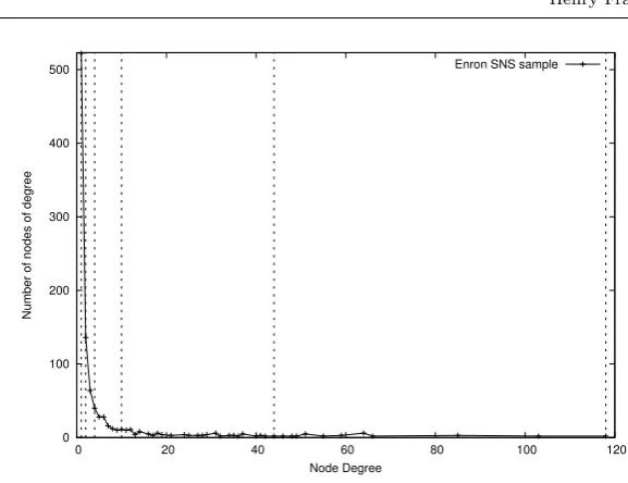
Fig. 1: Degree distribution of an Enron-SNS network sample, where the dotted lines denote the boundaries of each bin when applying our stratified sampling technique.
The main computational expense in our methodology is the calculation of topo-logical metrics for all agents inV and, if used, the influence model simulations for each location inS, which isO(|S||E|k), wherekis the number of simulation cycles. Depending on the size ofSthis can be significantly less than using the full network, which isO(|V||E|k). Additionally, Step 1 allows us to use a sample of the network to estimate influence, reducing the computational expense of the methodology. We recognise that the expense of computing location metrics is varied and might be high, and while we do not explicitly account for this within the methodology, we discuss local and approximation algorithms for our selected metrics in Section 4.
3.1 Selecting representative agent location samples
In order to effectively predict influence our methodology requires a sample of agents, S, that reflects the range of influence and topological metrics in the net-work. If the influence distribution is highly skewed then a random sample will not be representative (we discuss this further in Section 7). Therefore, we propose selecting a sample (in Step 2) by stratifying agents using degree. Since degree is known to be indicative of influence [5], our hypothesis is that this approach will give a more representative sample in terms of influence.
of the same degree to the same bin. We then sample an equal number of locations from each bin, until we have reached our required sample size,|S|. Note that given the long tail of the degree distribution it is possible for this approach to result in the locations being allocated to fewer than 10 bins if there are significantly more than|V|/10 locations in the first bin of lowest degree locations (or indeed in subsequent bins). The distribution and bin boundaries shown in Figure 1 are an illustration of this occurring, in which the approach results in 6 bins.
4 Topological metrics
In this section, we introduce the metrics that we hypothesise may aid in predicting agent influence, and discuss their computational tractability.
4.1 Metrics
There are a wide variety of metrics that quantify the structural properties of a given location in a network. Assuming a network,G < V, E >, and a given agent in the network located at nodevi∈V, we hypothesise that the following metrics
may be implicated in determining influence2.
1. Degree Centrality
If N(vi) denotes the set of neighbours for the agent located at vi, then
de-gree centralityki=|N(vi)|. Intuitively, the more agents that an individual can
directly communicate with, the more of the population that individual can di-rectly influence3. Degree centrality is trivial to compute with local information. 2. Local Clustering Coefficient (LCC)
The local clustering coefficient measures the extent to which the neighbours of
vi are connected to each other. Ifeij∈E denotes an edge betweenvi andvj,
where vi, vj∈V, then
LCC(vi) =
2|ejk|
ki(ki−1)
:vj, vk∈N(vi), ejk∈E
Initially introduced by Watts and Strogatz, LCC is a useful measure of com-munity structure in a network [49]. A individual at a location vi with a high
LCC is likely to be able to influence the local cluster in which it is embedded more effectively than individuals that are external to the cluster, and choices by neighbours ofvi are more likely to be reinforced byvi in subsequent
inter-actions.
3. Average Neighbour Degree (AND)
Average neighbour degree measures the average degree centrality of the neigh-bours of an agent. While a given agent may not be intrinsically influential
2 Note that for simplicity of presentation, and for consistency with the notation typically
used in network analysis, we use vi to denote the agent that is located at node vi in the network.
3 An intuition effectively encapsulated by the aphorism “It’s not what you know, but who
itself, communicating with a neighbouring influential neighbour may allow fur-ther opportunities for manipulating a population. We define AND as
AN D(vi) = P
vj∈N(vi)|N(vj)|
|N(vi)|
Average neighbour degree has not been investigated significantly. Liet al.have introduced a metric designed to measure the extent to which a network is scale-free [30], based on the Joint Degree Distribution (JDD), for which AND is an approximation [33], but we are not aware of other contributions considering the connectivity of neighbours of an agent at a given location.
4. Edge Embeddeddness and Overlap (EE/EO)
Edge embeddedness and overlap are two related measures that determine the extent to which the endpoints of an edge are embedded within a cluster of nodes [8]. Edge embeddedness for edge eij between agents located at nodesvi
andvj is defined as
EE(eij) =|N(vi) \
N(vj)|
Edge overlap is subsequently defined as
EO(eij) =
EE(eij)
|N(vi)SN(vj)|
Since these metrics are defined on a per-edge basis, we use three measures of each metric for a given location:
(a) Average (AEE/AEO): The average embeddedness or overlap will be high-est when an agent is highly embedded within a local cluster, providing opportunities to influence a small group of agents simultaneously.
(b) Highest (HEE/HEO): Taking the maximum embeddedness or overlap indi-cates whether an agent has any edges highly embedded within a cluster, while allowing for the agent itself to be connected to a wide variety of other agents or clusters.
(c) Lowest (LEE/LEO): An edge with low embeddedness or overlap may con-nect disparate clusters of agents, allowing the agents on each endpoint to influence across disparate communities in a network.
5. Average Shortest Path Length (ASPL)
Given a geodesic, or shortest, path between two locations vi, vj ∈V, defined
by a set of edges Espl(vi, vj) ∈ E, the average shortest path length for vi is
given by
ASP L(vi) = P
vj∈V\vi|Espl(vi, vj)|
|V| −1
Assuming that an agent’s influence diminishes as the number of hops increases, an agent with low ASPL may be able to indirectly influence a larger proportion of the population than an agent with a correspondingly higher ASPL. 6. Betweenness Centrality (BC)
Node centralities are a class of metrics that attempt to measure various facets of importance of a nodes in a network. The betweenness centrality ofvispecifically
σjk is the set of shortest paths that exist fromvj tovk, andσjk(vi) is the set
of shortest paths from vj tovk that pass throughvi, then
BC(vi) =
X
vi,vj,vk∈V,vi6=vj6=vk
|σjk(vi)|
|σjk|
Betweenness centrality is a useful measure of how much information is likely to flow through location vi, given that communications are likely to be along
shortest paths. As such, an agent with high betweenness has the ability to manipulate the information flow in a network more effectively than an agent with low betweenness.
7. Closeness Centrality (CC)
Closeness centrality is a measure of how quickly information can spread from a given agent. IfSP L(vi, vj) indicates the shortest path betweenviandvj, then
CC is calculated as
CC(vi) = P 1
vj∈V\vi|SP L(vi, vj)|
Since the assumption of information transfer following shortest paths may not hold in all domains, it may also be useful to calculate random walk centralities, which follow the identical definitions as above but use random walks instead of shortest paths. However, calculating these measures can be prohibitively expensive.
8. Eigenvector Centrality (EC)
Initially proposed by Bonacich, eigenvector centrality is calculated using the eigenvector of the largest eigenvalue given by the adjacency matrix representing the network in question [3]. An agent is central if it is connected to other agents that are central, and the measure takes into account both direct and indirect connections between agents. Google’s PageRank algorithm is a variant of EC, and this supports our intuition that EC may effectively estimate influence. Each entryavi,vj in the adjacency matrixAis 1 ifeij ∈Eand 0 otherwise. The
eigenvector centrality of an agent located at nodevi is subsequently calculated
as
EC(vi) = 1
λ
X
vj∈N(vi)
avi,vj×EC(vj)
where λis a constant.
9. Hyperlink-Induced Topic Search (HITS)
In total, we evaluate 14 metrics for the extent to which they determine agent in-fluence. Broadly, each metric can be linked to influence as follows. Eigenvector Cen-trality (EC), Betweenness CenCen-trality (BC), Closeness CenCen-trality (CC), Hyperlink-Induced Topic Search (HITS), and Average Shortest Path Length (ASPL) all measure the ability of an agent to manipulate information flow in a network. Lo-cal Clustering Coefficient (LCC), embeddedness, and overlap measure the extent to which an agent is part of a cluster of agents. Highly clustered areas of networks have efficient internal information propagation, and an agent that is very central to such a cluster is likely to be able to influence that cluster more effectively. Degree centrality is a measure of how many agents a given individual is able to directly influence, and Average Neighbour Degree (AND) is a measure of how many agents a given individual can indirectly influence to a depth of 2.
4.2 Computational tractability
While a number of these metrics are highly tractable, some of them require either, or both, of (i) global knowledge of the network, and (ii) significant computational resources. In typical on-line analysis of MAS networks these properties are unlikely to be attainable. The following discussion evaluates the computational costs and data requirements of each of our chosen metrics.
Degree, local clustering coefficient, edge embeddedness, edge overlap, and neigh-bour degrees are all easily computable with local knowledge. The most significant concerns are the centrality measures, which have typically required both global knowledge of the network and significant computational resources.
Edge betweenness is used in the Girvan and Newman (GN) algorithm for find-ing community structure [17]. Edge betweenness is a measure of the number of shortest paths between all nodes that contain a given edge, computable inO(mn) with global knowledge of a network withnnodes andmedges. Gregory proposed a local measure, h-betweenness, which only considers paths of maximum length
h[17]. Computation subsequently involves a breadth-first search (BFS) of depthh
around the node in question, and then computing betweenness on the BFS-sampled sub-graph. While Gregory provides strong results demonstrating the technique’s efficacy when substituted into the GN algorithm, there are no results on the ac-tual accuracy of the estimation. Marsden uses a similar technique [31], defining an egocentric betweenness centrality using the neighbours of a node, equivalent to 1-betweenness in Gregory’s measure. Marsden found that the ranking of nodes given by egocentric betweenness and the traditional global betweenness is very similar, but only evaluated fairly simple networks.
Andersen et al. have demonstrated a technique for calculating the PageRank of a node, which is a variant of Eigenvector Centrality (EC), using only local information [1]. The technique requires examination of O(e−1) nodes for a given error bound ofe. Interestingly, Andersenet al.note the potential of PageRank for approximating influence in a network [1].
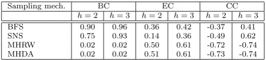
Table 1: Correlation between estimated centrality using Gregory’s h-betweenness concept and actual centrality for Betweenness Centrality (BC), and applying the technique to Eigenvector Centrality (EC) and Closeness Centrality (CC), averaged over 15 networks for selected network sampling techniques (see Section 5 for more details).
Sampling mech. BC EC CC
h= 2 h= 3 h= 2 h= 3 h= 2 h= 3
BFS 0.90 0.96 0.36 0.42 -0.37 0.41
SNS 0.75 0.93 0.14 0.36 -0.49 0.62
MHRW 0.02 0.02 0.50 0.61 -0.72 -0.74
MHDA 0.02 0.02 0.51 0.61 -0.73 -0.74
To our knowledge, there are no known local algorithms for HITS, but Gollapudi et al. have demonstrated a highly effective approximation algorithm for HITS-like ranking algorithms that demonstrates considerable efficiency gains [15]. The original proposal for HITS [26] calls for determining an initial seed set of around 200 nodes (in the context of finding pages on the World Wide Web), and then performing a limited snowball sampling (see Section 5) around this set. HITS does not require global knowledge of the network, but still has highly non-local information requirements.
We performed a series of tests for determining the accuracy of centrality estima-tion using Gregory’s h-betweenness technique [17]. For each locaestima-tion, we calculated the actual centrality measure and an estimation on the sub-graph induced by BFS around the location depth-limited to h={2,3}. Table 1 presents the correlation between the estimation and actual value. We used a selection of network sampling techniques to sample 15 networks of size 1000 from each of three real-world net-work datasets (see Section 5 for more details on the sampling mechanisms and network datasets used in this paper). Note that Gregory’s method was proposed only for betweenness-centrality, which shows the best correlations. The other cen-trality measures are included for completeness, but show much poorer estimation accuracy. For closeness centrality, this is by definition, since CC measures the in-verse of the sum of the shortest path length to all other locations, and withh= 2 the path length is either 1 or 2 for all locations. The technique used for sam-pling the network clearly has a significant impact on the efficacy of the estimation technique, implying that (i) estimating network measures in this way is highly sensitive to the local topological structure, and (ii) that each sampling technique reproduces unique subsets of the structural properties of the full network.
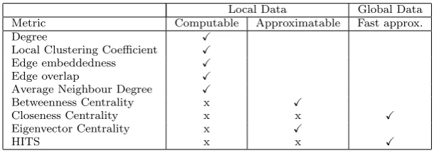
Table 2: Computational and information requirements for the calculation of each metric that we hypothesise might predict the influence of an agent at a given location. We denote the existence of a suitable algorithm with ‘X’, ‘x’ means that no known algorithm exists, and the blanks to the right of the table indicate that no algorithm is required (e.g. there is no need for an approximation if the solution is fully computable efficiently).
Local Data Global Data
Metric Computable Approximatable Fast approx.
Degree X
Local Clustering Coefficient X
Edge embeddedness X
Edge overlap X
Average Neighbour Degree X
Betweenness Centrality x X
Closeness Centrality x x X
Eigenvector Centrality x X
HITS x x X
Centrality), and the other (HITS) has an approximation using sampling a portion of the global network.
5 Network sampling
In this section, we discuss common approaches to sampling networks from real-world datasets. We analyse their efficacy in reproducing properties of the network being sampled, and describe the properties of networks sampled using each tech-nique from the datasets that we use in this paper. We assume that agents are arranged according to some underlying topology that restricts their communica-tions and interaccommunica-tions, and in the subsequent seccommunica-tions of this paper we will use such network samples to initialise the social relationships within populations of agents for our experiments.
5.1 Network sampling techniques
A wide variety of synthetic network generators have been proposed, but tend to be poor models of real-world networks [29, 37]. To demonstrate the applicability of our methodology, we require datasets representing networks found in real-world domains. Real-world networks typically exhibit two limiting properties: (i) they can be very large, beyond any size that is practically usable in a large number of simulations, and (ii) they contain a wide variety of rich structural properties that cannot be reproduced by current synthetic network generation algorithms (we demonstrate this in Section 7). We cannot typically expect to use global knowledge of the network to determine influential agents in practical applications. As such, sampling a portion of the network is often a necessary step in our methodology.
such as clustering coefficient or average degree, and other significant metrics such as degree distribution or edge embeddedness distribution.
There are a number of possible sampling techniques that can be used. Each starts at a random location, and progressively adds locations to a seed set until a threshold is reached.
1. Breadth-first search (BFS)
In each iteration of BFS, all the neighbours of seed set locations that are not already in the seed set are added, until the threshold is reached.
2. Snowball-sampling (SNS)
SNS proceeds identically to BFS, except within each iteration, if adding all the new neighbours to the seed set would push the set past the threshold, then neighbours are chosen randomly from those available until the sample size threshold is reached.
3. Random-walk (RW)
A random walk adds one location at a time to the seed set, by following a random traversal through the network from the start location. Each neighbour is chosen with uniform probability.
4. Metropolis-Hastings Random Walk (MHRW)
MHRW is a random-walk with transition probabilities biased away from high-degree locations, in an attempt to generate a uniform sampling (in terms of de-gree) of locations from the network. It was initially investigated in this context by Gjokaet al., who demonstrated that MHRW produces a uniform sampling of locations from the full network and effectively preserves the degree distri-bution [14], which is known to be a key component in the study of complex networks.
5. Metropolis-Hastings Random Walk with Delayed Acceptance (MHDA)
MHDA is the same as MHRW but with a further modification of transition probabilities to reduce the likelihood of re-visiting locations. Initially intro-duced by Lee et al., MHDA covers more of the network when sampling, in-creasing the estimation accuracy [28].
6. Albatross sampling
Introduced by Jin et al., Albatross sampling is a random walk with modified transition probabilities and a chance of randomly jumping to another location in the network, in order to gain greater coverage and avoid problems associated with sampling networks with multiple connected components [21].
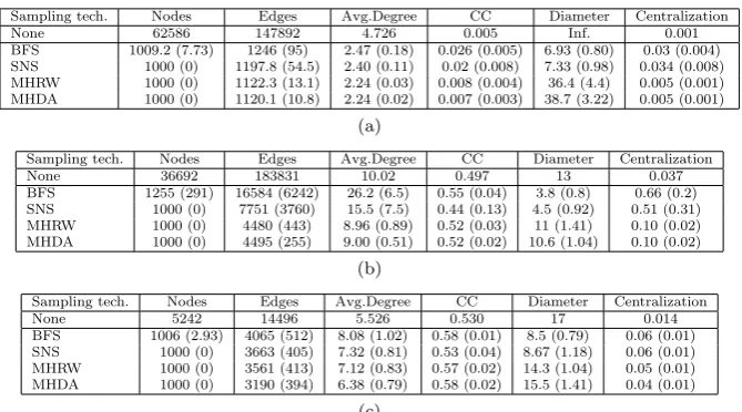
Table 3: Important global metrics for network samples produced by applying each sampling technique to the (a) Gnutella, (b) Enron, and (c) arXiv networks, aver-aged over 15 repeats. Standard deviation is in brackets.
Sampling tech. Nodes Edges Avg.Degree CC Diameter Centralization None 62586 147892 4.726 0.005 Inf. 0.001 BFS 1009.2 (7.73) 1246 (95) 2.47 (0.18) 0.026 (0.005) 6.93 (0.80) 0.03 (0.004) SNS 1000 (0) 1197.8 (54.5) 2.40 (0.11) 0.02 (0.008) 7.33 (0.98) 0.034 (0.008) MHRW 1000 (0) 1122.3 (13.1) 2.24 (0.03) 0.008 (0.004) 36.4 (4.4) 0.005 (0.001) MHDA 1000 (0) 1120.1 (10.8) 2.24 (0.02) 0.007 (0.003) 38.7 (3.22) 0.005 (0.001)
(a)
Sampling tech. Nodes Edges Avg.Degree CC Diameter Centralization None 36692 183831 10.02 0.497 13 0.037 BFS 1255 (291) 16584 (6242) 26.2 (6.5) 0.55 (0.04) 3.8 (0.8) 0.66 (0.2) SNS 1000 (0) 7751 (3760) 15.5 (7.5) 0.44 (0.13) 4.5 (0.92) 0.51 (0.31) MHRW 1000 (0) 4480 (443) 8.96 (0.89) 0.52 (0.03) 11 (1.41) 0.10 (0.02) MHDA 1000 (0) 4495 (255) 9.00 (0.51) 0.52 (0.02) 10.6 (1.04) 0.10 (0.02)
(b)
Sampling tech. Nodes Edges Avg.Degree CC Diameter Centralization None 5242 14496 5.526 0.530 17 0.014 BFS 1006 (2.93) 4065 (512) 8.08 (1.02) 0.58 (0.01) 8.5 (0.79) 0.06 (0.01) SNS 1000 (0) 3663 (405) 7.32 (0.81) 0.53 (0.04) 8.67 (1.18) 0.06 (0.01) MHRW 1000 (0) 3561 (413) 7.12 (0.83) 0.57 (0.02) 14.3 (1.04) 0.05 (0.01) MHDA 1000 (0) 3190 (394) 6.38 (0.79) 0.58 (0.02) 15.5 (1.41) 0.04 (0.01)
(c)
5.2 Technique efficacy
In order to evaluate the efficacy of each sampling technique, we sampled 15 graphs of 1000 nodes per sampling technique for each of three real-world networks (for a total of 180 networks). In this paper, we use the following networks: (i) a peer connection network from Gnutella (a P2P file-sharing platform), (ii) the Enron email dataset, and (iii) the arXiv general relativity section collaboration net-work4. The Enron and arXiv networks are both based on human interactions, but are generated by very different processes: the Enron dataset represents email communications, while arXiv is based on more formal links made through research collaborations. Conversely, Gnutella is a computational network representing links in a P2P system. Since these networks are generated by very different processes they display varied structural properties, allowing us to evaluate our methodol-ogy on a range of structures. The Gnutella and Enron networks are directed, but since MHRW and MHDA sampling explicitly only consider undirected networks, we treat each network as undirected.
The structural properties of these networks can be characterised by the high-level metrics shown in Table 3. The global clustering coefficient (GCC) is the average of the clustering coefficients for each node. Diameter describes the longest shortest path-length between a pair of nodes in the network. Centralization is a measure of how much heterogeneity exists in a graph [7]: if we define thedensity of a network of sizenas
Density= mean(k)
n−1
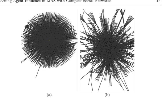
(a) (b)
Fig. 2: Structure of an example network sample produced by (a) Snowball sampling (SNS) and (b) MHRW sampling.
wherek denotes node degree, then we can define centralization as
Centralization= max(k)
n −Density
Centralization indicates the extent of variation of node degree in the network, with a low centralization indicating that most nodes have a similar connectivity, whereas high centralization implies a higher degree of structural variation throughout the network. While this measure is mainly practically applied in biological studies, it is useful here as an indication of the extent to which a mechanism has generated a uniform sample.
From examination of the data in Table 3, we can see that no single technique produces an ideal sample. As discussed above, BFS and SNS are known to be highly biased towards high-degree nodes, but produce good coverage of localised areas in a network. The standard deviation between individual samples is highest using these techniques, indicating a large variation in structural properties between samples. The centralisation is also very high using BFS and SNS, indicating that a much higher level of internal hetereogeneity is introduced by using these sampling techniques. MHRW and MHDA tend to have the lowest standard deviation be-tween samples, and produce networks with metric values such as average degree, clustering coefficient and centralisation much closer to the full network than SNS and BFS. However, the diameter of the MHRW and MHDA samples is far higher than with SNS and BFS, which we hypothesise is due to the random walk nature of these techniques covering large areas of the network. Given that these sampled networks clearly no longer display the small-world property, we cannot assert that many of the structural properties of the full network are reproduced, beyond the node degree distribution.
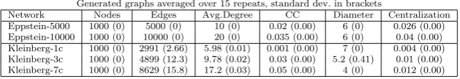
Table 4: Important global metrics for networks produced by the Eppstein and Kleinberg network generators, averaged over 15 repeats. Standard deviation is in brackets. For the Eppstein networks, the number annotation indicates the number of edges. For the Kleinberg networks, the “-xc” annotation indicates the additional number of extra connections x(a parameter to the algorithm) that was used to generate the network.
Generated graphs averaged over 15 repeats, standard dev. in brackets
Network Nodes Edges Avg.Degree CC Diameter Centralization Eppstein-5000 1000 (0) 5000 (0) 10 (0) 0.02 (0.00) 6 (0) 0.026 (0.00) Eppstein-10000 1000 (0) 10000 (0) 20 (0) 0.035 (0.00) 6 (0) 0.04 (0.00) Kleinberg-1c 1000 (0) 2991 (2.66) 5.98 (0.01) 0.001 (0.00) 7 (0) 0.004 (0.00) Kleinberg-3c 1000 (0) 4899 (12.3) 9.78 (0.02) 0.03 (0.00) 5.2 (0.41) 0.01 (0.00) Kleinberg-7c 1000 (0) 8629 (15.8) 17.2 (0.03) 0.05 (0.00) 4 (0) 0.012 (0.00)
perhaps indicating that SNS is slightly less biased towards high degree nodes. However, SNS can often produce distorted network structures depending on the initial node chosen. Figure 2a shows a SNS network sample where the first node sampled has a very large degree, resulting in a star-shaped sample with unrep-resentative node degree distribution and clustering coefficient. Figure 2b shows a MHRW sample of the same network, clearly showing a more homogeneous network structure.
If we are to claim that our methodology is effective in a general sense, we must be careful to analyse agent populations that are situated upon as many network structures as possible. We believe that the best approach is to use a portfolio of network samples derived using a variety of sampling techniques. Using BFS or SNS allows us to apply our methodology on samples that are more representative of localised areas of the full network, and the higher variance between samples indicates a wider variety of structural properties will be analysed. Given that there is little consistent difference between BFS and SNS, for simplicity in the remainder of this paper we use SNS as a sampling method for retaining a representation of local structure. Using MHRW or MHDA allows analysis of samples in which we can be sure that the node degree distribution is closer to that of the full network, but we cannot make any assertions about other properties. Given that the diameter is so much larger in network samples produced using these techniques, it is likely that there are other as-yet undocumented biases introduced.
Therefore we sample, from each of the Gnutella, Enron, and arXiv datasets, 5 network samples using SNS, 5 network samples using MHRW, and 5 network sam-ples using MHDA, making a total of 45 networks with which to test our method-ology. These network samples are used to configure our simulations, such that the network topology determines the set of neighbours for each individual agent in the population. We also initially include a number of synthetic networks for comparison, as follows.
1. Scale-free networks generated using the Eppstein power-law generation algo-rithm [9]. We use two Eppstein power-law networks generated with 1000 nodes, and 5000 and 10000 edges respectively.
Comparing the properties of the real-world networks (Table 3) with the syn-thetic network properties in Table 4 illustrates the significant differences between the real-world and synthetic networks. This is best demonstrated by inspecting the clustering coefficient, which is far higher in real-world networks. This is in-dicative of the structural differences between these networks and the insufficiency of common network generation algorithms in modelling real-world domains. The synthetic generation algorithms produce consistently structurally similar graphs. For example, over 200 generated Eppstein power-law networks, using identical con-figurations, the standard deviation for node degree is 0 and the standard deviation for clustering coefficient is 0.001.
6 Experimental setup
To evaluate our methodology for learning influence, as described in Section 3, we use two major models of convention emergence in complex open MAS, namely, Salazar et al.’s language coordination domain [40], and the coordination game (described, for example, in [42]). In each experiment, we insert a single fixed-strategy Influencer Agent (IA) [13] at a randomly chosen location, and measure the extent to which the population converges on the strategy of the IA.
We apply our methodology as follows. From each of the Gnutella, Enron and arXiv networks described above, we sample 45 sub-networks of 1000 nodes using the SNS, MHRW and MHDA network sampling methods, and use these network samples to initialise a population of 1000 agents (Step 1 of our methodology). We then sample 50 locations, using either random or stratified-by-degree sampling (Step 2), and run our simulation 20 times for each location, giving a total of 1000 simulation runs per sub-network. We select an appropriate measure of influence for the interaction domain used (Step 3), as discussed later in this section. After each simulation, we measure the extent to which the agent at this location influenced the rest of the population, and calculate each of the fourteen topological location metrics (introduced in Section 4) for that location (Step 4). We then calculate the topological location metrics for all agents in the population (Step 5). Finally, we use machine learning techniques to build a prediction model using the topological location metrics to estimate the influence of all agents in the population (Step 6). In this paper, our focus is on the methodology itself and the identification of appropriate location metrics, and so we build simple prediction models using Principal Components Analysis (PCA) for unsupervised learning and Linear Re-gression (LR) for supervised learning. To evaluate our approach, we then run new simulations using the location predicted as most influential by each model, and determine the extent to which influence has increased.
We use the Java Universal Network/Graph Framework5 in our simulations and Cytoscape6for off-line structural analysis of networks. Statistical analyses are performed using R7and Weka8.
5 http://jung.sourceforge.net/ 6 http://www.cytoscape.org/ 7 http://www.r-project.org/
6.1 Language coordination domain
The first domain that we use to learn agent influence is the language coordination domain introduced by Salazaret al., in which agents are associated with a lexicon that mapswords toconcepts [40]. We use Salazaret al.’s parameter settings of 10 concepts and 10 words, with 10 mappings per lexicon (giving a convention space of size 1010) [40]. Each timestep, three phases are executed. First, each agent in turn communicates a single mapping from its lexicon to a single randomly chosen neighbour. It is assumed that agents can determine whether the recipient’s lexicon contains the same mapping, in which case the communication issuccessful, other-wise it is unsuccessful. Second, each agent has a chance to propagate part of its lexicon to all of its neighbours, along with thecommunicative efficacyof the lexicon, defined as the proportion of successful communications in the last 20 communi-cations. Third, each agent has a chance to update their internal lexicon based on the partial lexicons received from their neighbours, using a two-point crossover. Agents use anelitiststrategy, such that they update their lexicon with the received mappings that have the highest communicative efficacy. It is important to note that since agents only communicate a single mapping from the 10 in their lexicon there is a significant level of partial observability in this domain. When updating their mappings agents are subject to this partial observability, since they are only able to adopt the single mapping that was communicated, with the remaining 9 mappings used by the sending agent being unknown.
Over time a shared lexicon, a set of mappings from words to concepts, emerges. We run each simulation for 50000 timesteps, and each agent propagates their lexicon with a probability of 0.01 and updates their lexicon with a probability of 0.01. By the end of a typical simulation run 600–800 agents have adopted the dominant lexicon.
In this domain, we define an agent’sinfluence (Step 3 of our methodology) as the similarity between its lexicon (L) and final dominant lexicon in the population (L0) using Jaccard’s similarity coefficient, J(L, L0) = |L∩L0|/|L∪L0|, where a similarity of 1 implies that agents use an identical lexicon, and 0 implies there are no mappings in common.
6.2 Coordination game domain
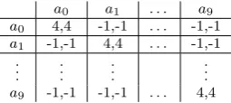
To corroborate our results in the language coordination domain, we use a model of convention emergence loosely based on Sen and Airiau’s private learning [42] and Walker and Wooldridge’s model of convention emergence with local informa-tion [46], with modificainforma-tions. Each timestep, every agent in turn engages in an interaction with a randomly chosen neighbour, using a coordination game with ten possible action choices (see Table 5 for the payoff structure). Since social im-itation and information propagation are fundamental processes in the emergence of conventions, we split strategy selection for each agent into two mechanisms: (i) personal, based on the individual’s direct interaction history, and (ii)social, based on the interactions an individual has observed. When selecting a strategy, agents choose uniformly at random between personal and social choices.
het-Table 5: Payoff structure for the 10-action coordination game, showing the payoffs received by agents for a given combination of actions, whereairepresents actioni,
andx, yrepresents the payoffs received by the row and column players respectively.
a0 a1 . . . a9
a0 4,4 -1,-1 . . . -1,-1
a1 -1,-1 4,4 . . . -1,-1
. . .
. . .
. . .
. . .
a9 -1,-1 -1,-1 . . . 4,4
erogeneity, we use a variety of strategy selection mechanisms. For personal expe-rience, agents learn using either a Q-learning algorithm [47] or WoLF-PHC [4]. When selecting a strategy based on social experience, an agent learns using either Q-learning, WoLF-PHC, Highest Cumulative Reward (HCR) [43], or Most Re-cently observed (MR). At the start of the simulation, each agent is initialised with a mechanism for personal and a mechanism for social choice chosen uniformly at random, giving a total of 8 possible agent configurations. Agents explore in 10% of interactions by selecting a strategy uniformly at random. This exploration intro-duces a significant level of noise into our simulations, since 10% of the time agents select actions randomly rather than according to their true strategy, which in turn provides noisy information on which their interaction partner will learn.
The ideal goal is for the population to converge to a state in which every agent selects the same strategy, resulting in population-wide coordination. In practice, we find that around 3 or 4 strategies persist as co-existing conventions, each having similar numbers of adherents. We define a “win” as a simulation run in which the dominant strategy (i.e. the strategy or lexicon with the highest number of adherents) is that used by the IA, and use the normalised number of wins over 20 simulation repeats as our metric of influence (Step 3 of our methodology). Due to the co-existence of conventions with similar adherence numbers, the exploration of agents, and the higher possibility of a win being the result of chance, influence is harder to measure accurately in this setting than in the language coordination domain. Since the classification of whether an agent adheres to a convention relies on the agent’s interaction history, convention memberships are volatile over time which introduces noise into the measure of whether an agent has been influenced.
7 Results
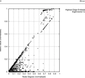
[image:20.595.181.309.141.198.2]0 0.2 0.4 0.6 0.8 1
0 0.1 0.2 0.3 0.4 0.5 0.6 0.7 0.8 0.9 1
Metric value (normalised)
Node Degree (normalised)
[image:21.595.76.364.68.331.2]Highest Edge Embeddedness Eigenvector Centrality HITS
Fig. 3: Correlation of HEE, EC, and HITS with node degree in an example arXiv-SNS network sample.
7.1 Targeting IAs using individual metrics
Inspecting the extent to which individual metrics predict influence may allow us to refine our models, and analysis of the correlations between each metric and influence reveals that Degree, EC, HEE, and HITS all robustly correlate with influence over all networks. These metrics are statistically significantly correlated in over 90% of the networks (with correlations ranging from 0.68 in the arXiv networks to 0.27 in the Enron networks), whereas the other metrics statistically significantly correlate only in isolated networks (on average, in 48% of networks). Correlating with influence in isolated networks is likely to be due to unique network structures, and these metrics are less likely to indicate influential agents in the general case. This corroborates previous research on the link between degree and influence (e.g. [5]), but to our knowledge this is the first time that EC, HEE and HITS have been shown to predict influence.
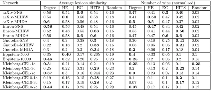
Table 6: Average lexicon similarity and number of wins for placing a single fixed-strategy agent (IA) either at a location maximising one of the chosen metrics or randomly in the language coordination domain. The best performing placement strategies are in bold. In the Kleinberg networks, the “CE” annotation indicates the clustering exponent (a parameter of the algorithm) used to generate the net-work.
Network Average lexicon similarity Number of wins (normalised) Degree HE EC HITS Random Degree HE EC HITS Random arXiv-SNS 0.58 0.54 0.6 0.54 0.16 0.47 0.41 0.5 0.40 0.03 arXiv-MHRW 0.54 0.6 0.56 0.58 0.18 0.41 0.50 0.47 0.42 0.02 arXiv-MHDA 0.6 0.58 0.56 0.48 0.16 0.5 0.5 0.47 0.37 0.02 Enron-SNS 0.58 0.56 0.48 0.54 0.16 0.45 0.47 0.34 0.42 0.02 Enron-MHRW 0.62 0.48 0.55 0.63 0.16 0.55 0.41 0.44 0.56 0.02 Enron-MHDA 0.56 0.58 0.6 0.6 0.16 0.47 0.47 0.6 0.6 0.02 Gnutella-SNS 0.4 0.3 0.38 0.5 0.18 0.30 0.18 0.25 0.41 0.06 Gnutella-MHRW 0.22 0.18 0.2 0.38 0.16 0.08 0.05 0.06 0.21 0.02 Gnutella-MHDA 0.3 0.2 0.3 0.34 0.18 0.2 0.06 0.17 0.18 0.04 Eppstein-5000 0.35 0.40 0.17 0.265 0.19 0.4 0.33 0.05 0.1 0.1 Eppstein-10000 0.46 0.32 0.20 0.25 0.23 0.25 0.2 0.05 0.2 0.15 Kleinberg-CE1-1c 0.31 0.21 0.14 0.2 0.19 0.25 0.13 0.05 0.1 0.25 Kleinberg-CE1-3c 0.25 0.22 0.31 0.29 0.23 0.2 0.13 0.2 0.23 0.14 Kleinberg-CE1-7c 0.37 0.3 0.16 0.244 0.23 0.3 0.23 0.07 0.13 0.14 Kleinberg-CE10-1c 0.19 0.16 0.15 0.28 0.27 0.1 0.1 0.1 0.2 0.1 Kleinberg-CE10-3c 0.15 0.17 0.19 0.28 0.2 0.07 0.1 0.1 0.17 0.12 Kleinberg-CE10-7c 0.44 0.17 0.25 0.26 0.29 0.37 0.17 0.17 0.1 0.12
Table 6 shows the average lexicon similarity and the number of wins for placing an IA at the location that maximises each metric, where a win is defined as a simulation run in which the dominant lexicon in the population has at most 2 different mappings from the IA lexicon. Results are averaged over each class of network sample. We see significant gains across all four metrics, particularly in the arXiv and Enron networks. With random placement, an agent is only able to successfully influence the population 2 times in 100, but placing by metric can increase this to 60 times in 100. There is no consistency in which metric performs best across network samples, and this is likely to be due to unique network structures in each class of network.
The synthetic networks show very few gains in influence using targeted place-ment, and very few of the metrics significantly correlate with influence for these networks. We believe that the networks generated by current synthetic generation algorithms are too homogeneous for any given location to gain significant influence over others, and our results demonstrate that, since the potential for influence is so much lower, the synthetic networks used here are poor models of networks found in the real world. Accordingly, we focus only on the real-world network samples for the remainder of this paper.
7.2 Targeting IAs using learnt models
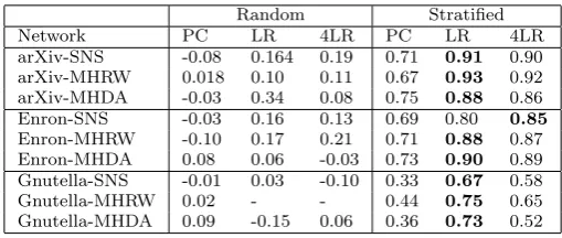
pre-Table 7: Correlation of each learnt model with measured influence in the language coordination game, using separate training and test data, over each class of network sample and learnt on both random and stratified sampling. Entries shown in bold indicate the highest correlation for that network sample.
Random Stratified
Network PC LR 4LR PC LR 4LR
arXiv-SNS -0.08 0.164 0.19 0.71 0.91 0.90
arXiv-MHRW 0.018 0.10 0.11 0.67 0.93 0.92
arXiv-MHDA -0.03 0.34 0.08 0.75 0.88 0.86
Enron-SNS -0.03 0.16 0.13 0.69 0.80 0.85
Enron-MHRW -0.10 0.17 0.21 0.71 0.88 0.87
Enron-MHDA 0.08 0.06 -0.03 0.73 0.90 0.89
Gnutella-SNS -0.01 0.03 -0.10 0.33 0.67 0.58
Gnutella-MHRW 0.02 - - 0.44 0.75 0.65
Gnutella-MHDA 0.09 -0.15 0.06 0.36 0.73 0.52
diction performance that is comparable or approaching that obtained with the full linear regression, while having reduced computational overhead. We consider two sampling approaches for selecting a representative set of locations (i.e. Step 2 of our methodology): random and stratified location sampling (as described in Section 3).
We trained our model as follows. For each combination of sampling technique (i.e. SNS, MHRW and MHDA) and network (i.e. arXiv, Enron, Gnutella), there are five network samples, from which 50 locations are selected for IA placement either randomly or using stratification. We use a cross-fold validation approach by dividing the data on how influential each location is in each network sample into four network samples for training, and one network sample for testing, for each possible combination of the five networks in each configuration. Once trained, we measured the correlation between the predicted influence and measured influence for the test data (to gain an estimation of the accuracy of our technique). Finally, we train the model on all available data for a network sample, and use it to predict which locations might be most influential. We evaluate this prediction by running simulations with an IA at the location predicted as maximising influence.
[image:23.595.118.373.143.251.2]0 10000 20000 30000 40000 50000 60000 70000 80000
0 100 200 300 400 500 600 700 800 900 1000
Predicted influence
[image:24.595.74.419.74.328.2]Agents
[image:24.595.73.417.423.529.2]Fig. 4: Predicted influence for each agent in an example SNS sample from the arXiv network.
Table 8: Average lexicon similarity and normalised number of wins when placing an IA at a location chosen by the predictive models in the language coordination domain. The best performing placement strategies are shown in bold.
Network Average lexicon similarity Number of wins (normalised)
PC LR 4LR Random PC LR 4LR Random
arXiv-SNS 0.44 0.42 0.58 0.16 0.34 0.30 0.50 0.03
arXiv-MHRW 0.5 0.32 0.62 0.18 0.42 0.20 0.55 0.02
arXiv-MHDA 0.34 0.38 0.6 0.16 0.22 0.27 0.50 0.02
Enron-SNS 0.62 0.32 0.68 0.16 0.56 0 0.62 0.02
Enron-MHRW 0.2 0.5 0.58 0.16 0.30 0.36 0.53 0.02
Enron-MHDA 0.34 0.16 0.52 0.16 0.21 0.06 0.43 0.02
Gnutella-SNS 0.18 0.46 0.36 0.18 0.03 0.37 0.24 0.06
Gnutella-MHRW 0.4 0.4 0.24 0.16 0.27 0.29 0.10 0.02
Gnutella-MHDA 0.38 0.36 0.36 0.18 0.25 0.24 0.22 0.04
from stratified sampling, indicating that random sampling of locations does not give a sufficient range of influential locations to learn accurate models.
Targeting IAs using locations predicted as influential by learnt models based on stratified data results in significant gains in influence. In the arXiv, Enron and Gnutella-SNS network samples, these increases are roughly equal to that gained through placing by single metric over random placement. In the arXiv and En-ron network samples, the best performing model is 4LR, indicating that the other metrics are unlikely to contribute significantly to influence prediction. We believe that 4LR is learningwhich metric is best to place by, given the results in Table 6, since the results from placing by 4LR are roughly equivalent to placing by thebest performing metric (out of the four) for each network sample. In Gnutella, 4LR is always outperformed by PC or LR, indicating that metrics other than Degree, EC, HEE and HITS are indicative of influence in these networks. Moreover, the linear combination of metrics in each of these network samples outperforms place-ment by single metrics. The Gnutella network samples show a reduced potential for influence compared to the samples from the Enron and arXiv networks, and exhibit lower edge counts, average degree, and clustering coefficients, and higher diameters. All these properties reduce the ability of an agent to exert influence, and may provide an indication of the likely efficacy of our methodology prior to application.
Our results suggest that if computational expense is an issue, targeting by Degree (or EC, HEE or HITS) will yield significant gains in influence, but if computational expense is less important, then applying our methodology results in further gains. If our methodology is applied using online measurements of influence (i.e. not requiring repeated simulations), the computational cost is significantly reduced.
7.3 Targeting IAs in the coordination game
The results given above suggest that agents can attain significant gains in influence by exploiting knowledge of the topological structure connecting agents. However, we have so far only considered results for the language coordination domain, and to demonstrate generality it is necessary to test the extent to which agents can gain influence from targeting placement according to a prediction model based on topological characteristics in another agent interaction regime. Accordingly, in this section we present results from targeting IAs within the coordination game described in Section 6.2. We initially target locations predicted as influential by each of the four single metrics previously identified in Section 7.1. We build new prediction models with data generated from running coordination game simula-tions for the same (stratified by degree) location sets as those used in Section 7.2. This allows us to directly compare the quality of models learnt using different agent interaction processes and metrics of influence. In contrast, in Section 7.4 we use the actual prediction models learnt in the language coordination domain (Section 7.2) to predict influence in the coordination game domain, and vice versa, to determine the extent to which these models predict influence across domains.
Table 9: Normalised number of wins when placing an IA at a location selected by maximising each of the four single metrics identified in Section 7.1 in the coordination game. The best performing metrics are highlighted in bold.
Network Number of wins (normalised)
Degree HEE EC HITS Random
arXiv-SNS 0.43 0.33 0.41 0.40 0.11
arXiv-MHRW 0.39 0.35 0.40 0.36 0.10
arXiv-MHDA 0.43 0.42 0.38 0.33 0.09
Enron-SNS 0.38 0.40 0.33 0.38 0.10
Enron-MHRW 0.45 0.39 0.37 0.47 0.10
Enron-MHDA 0.42 0.38 0.48 0.48 0.09
Gnutella-SNS 0.28 0.23 0.23 0.35 0.09
Gnutella-MHRW 0.18 0.12 0.15 0.18 0.12
[image:26.595.142.347.299.407.2]Gnutella-MHDA 0.12 0.23 0.25 0.18 0.08
Table 10: Normalised number of wins when placing an IA at a location chosen by the predictive models using the coordination game. The best performing placement strategies are shown in bold.
Network Number of wins (normalised)
PC LR 4LR Random
arXiv-SNS 0.13 0.16 0.25 0.11
arXiv-MHRW 0.18 0.14 0.26 0.10
arXiv-MHDA 0.17 0.12 0.22 0.09
Enron-SNS 0.10 0.13 0.23 0.10
Enron-MHRW 0.12 0.10 0.24 0.10
Enron-MHDA 0.11 0.14 0.23 0.09
Gnutella-SNS 0.13 0.17 0.15 0.09
Gnutella-MHRW 0.23 0.19 0.15 0.12
Gnutella-MHDA 0.19 0.16 0.13 0.08
in influence while the Gnutella samples exhibit relatively small gains. The gains in influence are not as large as in the language coordination domain and this is likely to be because the combination of multiple co-existing conventions with similar numbers of adherents, agent exploration, and reduced size of the convention space result in a domain in which influencing the population is more difficult. It may also be that the scope for influence, as imbued purely by network structure, is reduced in this domain simply due to its inherent mechanisms. Nonetheless, there is still clearly potential for targeting individual locations for gains in influence.
Furthermore, there are only ten discrete strategies in the coordination game domain, and switching strategies can involve non-trivial costs. In particular, given that a number of conventions co-exist with similar membership sizes, an agent being influenced to a given strategy can directly result in subsequent costs if that agent interacts with a neighbour adhering to a different convention. In the language coordination domain, the convention space is quasi-continuous and switching con-vention is less likely to incur costs (consider that if an agent alters one mapping in a lexicon, that mapping may not be used in a communication for some time). This leads to two effects: (i) agents are less likely to incur costs as a result of altering convention in the language coordination domain, leading to increased likelihood of being successfully influenced (as opposed to being influenced, incurring a cost and switching to another strategy), and (ii) in the coordination game domain the methodology has to learn on the number of absolute wins, rather than the more fine grained measure of lexicon distance. As a result of the second issue, the learning algorithms have less detailed data on which to learn, further reducing the efficacy of the methodology.
7.4 Using learnt models in other domains
A major component of our hypothesis regarding the poorer results in the coordi-nation game domain is that the data available is less suitable for accurate learning. To test this, we performed two sets of experiments. Firstly, we re-ran simulations in the coordination game domain, but placed IAs at the position predicted as most influential by the models learnt using data from the language coordination domain, which had resulted in models that appeared to predict more influential locations. Secondly, we ran simulations in the language coordination domain, with IAs placed at locations predicted as most influential by the models learnt using data from the coordination game domain.
Table 11 plots the normalised number of wins attained in the first set of ex-periments (i.e. running simulations in the coordination game domain with models learnt on data from the language coordination domain). We can clearly see that using these models does result in gains in influence, despite using a model learnt on data from a different domain. This suggests that (i) the models learn intrinsic influence relating to the network structure itself, rather than as a result of the specific behavioural patterns exhibited by agents situated on the network, and (ii) that, to some extent, these models can be used to predict influence even when the behaviour of agents in the targeted domain is significantly different to that used to generate the data from which the model is built. Note that there is far higher variation in the results, especially with respect to the Enron network sam-ples. We believe this to be a result of the coordination game domain itself having far higher variation in the outcomes of individual simulation runs. The Gnutella network samples display inconsistent behaviour in terms of which learnt models are best, and the learnt models appear to have fairly similar predictive power in this context.
Table 11: Normalised number of wins gained by placing an IA at a location cho-sen by the predictive models learnt on the language coordination data, using the coordination game. The best performing placement strategies are shown in bold.
Network Number of wins (normalised)
PC LR 4LR Random
arXiv-SNS 0.3 0.21 0.37 0.11
arXiv-MHRW 0.16 0.19 0.35 0.10
arXiv-MHDA 0.16 0.15 0.30 0.09
Enron-SNS 0.40 0.14 0.76 0.10
Enron-MHRW 0.28 0.45 0.26 0.10
Enron-MHDA 0.15 0.15 0.55 0.09
Gnutella-SNS 0.11 0.1 0.36 0.09
Gnutella-MHRW 0.19 0.13 0.19 0.12
Gnutella-MHDA 0.19 0.21 0.20 0.08
language coordination domain targeted using models learnt on data from the same domain. The average gain in lexicon similarity is statistically indistinguishable whether IAs are targeted using models learnt on language coordination domain data or coordination game domain data.
When using the coordination game domain, using predictive models trained on data gathered in different agent-interaction models appears to incur a cost in terms of IA efficacy. When using the language coordination domain, models trained on data from different agent-interaction models are as effective as models trained on data from the same agent-interaction model as that being tested. The mechanism behind this discrepancy is unclear. There may be some property of an agent-interaction model that imparts greater generality to the predictive models learnt on their data, or features of a particular domain, such as a richer relationship between conventions, may make it more amenable to influence. In future work, we will extend these experiments to a wider set of agent-interaction models to determine to what extent, in general, predictive models can be translated between domains.
Overall, we can conclude that learnt models for predicting influence from topo-logical metrics, for the large part, do translate between the different interaction domains considered in this paper. If a target domain does not have easily defin-able on-line influence metrics or off-line agent models, it may therefore be possible to use a simple interaction domain, such as the language coordination setting, to generate data on which to apply our methodology and still retain significant efficacy.
7.5 Prediction comparison
Table 12: Average lexicon similarity and normalised number of wins when placing an IA, in the language coordination domain, at a location chosen by predictive models learnt on data from the coordination game domain. The best performing placement strategies are shown in bold.
Network Average lexicon similarity Number of wins (normalised)
PC LR 4LR Random PC LR 4LR Random
arXiv-SNS 0.46 0.46 0.52 0.16 0.36 0.33 0.42 0.03
arXiv-MHRW 0.52 0.32 0.68 0.18 0.41 0.18 0.59 0.02
arXiv-MHRWDA 0.50 0.32 0.61 0.16 0.41 0.19 0.53 0.02
Enron-SNS 0.64 0.63 0.51 0.16 0.46 0.5 0.51 0.02
Enron-MHRW 0.48 0.52 0.38 0.16 0.36 0.44 0.27 0.02
Enron-MHRWDA 0.14 0.24 0.6 0.16 0.0 0.08 0.51 0.02
Gnutella-SNS 0.16 0.4 0.36 0.18 0.02 0.29 0.25 0.06
Gnutella-MHRW 0.42 0.36 0.26 0.16 0.3 0.25 0.15 0.02
Gnutella-MHRWDA 0.4 0.34 0.2 0.18 0.24 0.24 0.07 0.04
Network Predictive model
PC LR 4LR
arXiv-SNS 0.0 1.0 0.6
arXiv-MHRW 0.6 1.0 1.0
arXiv-MHRWDA 0.0 0.0 1.0
Enron-SNS 1.0 0.0 0.0
Enron-MHRW 0.0 1.0 1.0
Enron-MHRWDA 0.0 0.8 0.8
Gnutella-SNS 0.0 1.0 1.0
Gnutella-MHRW 1.0 1.0 1.0
Gnutella-MHRWDA 0.0 1.0 0.6
Table 13: Table showing, for each class of networks and model type, the proportion of networks for which the same location was predicted as most influential by (i) a model learnt on results from 50 locations selected by stratified sampling and (ii) a model learnt on the same results as (i) plus results from placing a single IA at the location predicted as most influential by (i). If both models predict the same location, then this strengthens the evidence supporting the accuracy of the first model.
model from (i). If the models disagree, then the new data from the targeted IA has altered the model sufficiently to change which location is predicted as most influential, suggesting that the original model was not accurate. Conversely, if they agree, then this suggests that the original model was a reasonably good model for predicting influence.