warwick.ac.uk/lib-publications
Copyright and reuse:
The Warwick Research Archive Portal (WRAP) makes this work by researchers of the
University of Warwick available open access under the following conditions. Copyright ©
and all moral rights to the version of the paper presented here belong to the individual
author(s) and/or other copyright owners. To the extent reasonable and practicable the
material made available in WRAP has been checked for eligibility before being made
available.
Copies of full items can be used for personal research or study, educational, or not-for-profit
purposes without prior permission or charge. Provided that the authors, title and full
bibliographic details are credited, a hyperlink and/or URL is given for the original metadata
page and the content is not changed in any way.
Publisher’s statement:
This article has been accepted for publication in Monthly Notices of the Royal Astronomical
Society ©: 2016 The Authors Published by Oxford University Press on behalf of the Royal
Astronomical Society. All rights reserved.
A note on versions:
The version presented in WRAP is the published version or, version of record, and may be
cited as it appears here.
6Instituto de Astrof´ısica de Canarias, V´ıa Lactea s/n, La Laguna, E-38205 Tenerife, Spain
7Astrophysics Research Institute, Liverpool John Moores University, IC2, Liverpool Science Park, 146 Brownlow Hill, Liverpool L3 5RF, UK 8Millenium Nucleus ‘Protoplanetary Disks in ALMA Early Science’, Universidad de Valparaiso, Valparaiso 2360102, Chile
Accepted 2016 March 1. Received 2016 March 1; in original form 2015 November 16
A B S T R A C T
We present high-speed photometry and high-resolution spectroscopy of the eclipsing post-common-envelope binary QS Virginis (QS Vir). Our Ultraviolet and Visual Echelle Spectro-graph (UVES) spectra span multiple orbits over more than a year and reveal the presence of several large prominences passing in front of both the M star and its white dwarf companion, allowing us to triangulate their positions. Despite showing small variations on a time-scale of days, they persist for more than a year and may last decades. One large prominence extends almost three stellar radii from the M star. Roche tomography reveals that the M star is heavily spotted and that these spots are long-lived and in relatively fixed locations, preferentially found on the hemisphere facing the white dwarf. We also determine precise binary and physical pa-rameters for the system. We find that the 14 220±350 K white dwarf is relatively massive, 0.782±0.013 M, and has a radius of 0.010 68±0.000 07 R, consistent with evolutionary models. The tidally distorted M star has a mass of 0.382±0.006 Mand a radius of 0.381± 0.003 R, also consistent with evolutionary models. We find that the magnesium absorption line from the white dwarf is broader than expected. This could be due to rotation (implying a spin period of only∼700 s), or due to a weak (∼100 kG) magnetic field, we favour the latter interpretation. Since the M star’s radius is still within its Roche lobe and there is no evidence that it is overinflated, we conclude that QS Vir is most likely a pre-cataclysmic binary just about to become semidetached.
Key words: binaries: eclipsing – stars: fundamental parameters – stars: late-type – white dwarfs.
1 I N T R O D U C T I O N
Close binaries containing a white dwarf and a low-mass M star are survivors of a common envelope phase of evolution during which both stars orbited within a single envelope of material ejected by the progenitor of the white dwarf. These systems slowly lose angular momentum via gravitational radiation and (if the M star is massive enough) magnetic braking, eventually becoming semi-detached cataclysmic variable (CV) systems.
E-mail:[email protected]
In recent years, the number of such systems known has dramat-ically increased, thanks mainly to the Sloan Digital Sky Survey (SDSS; York et al.2000; Adelman-McCarthy et al.2008; Abaza-jian et al. 2009), which has led to the discovery of more than 2000 white dwarf plus main-sequence systems (Rebassa-Mansergas et al. 2013b), from which more than 200 close, post-common-envelope binaries (PCEBs) have been identified (Nebot G´omez-Mor´an et al.2011; Parsons et al.2013a,2015). Among this sam-ple are 71 eclipsing binaries (see the appendix of Parsons et al. 2015for a recent census). These are extremely useful systems for high-precision stellar parameter studies, since the small size of the white dwarf leads to very sharp eclipse profiles, allowing radius
at University of Warwick on October 24, 2016
http://mnras.oxfordjournals.org/
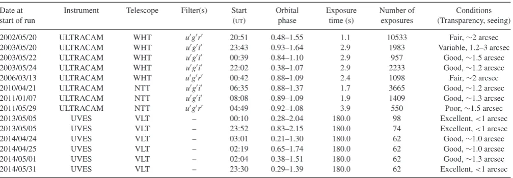
2014/05/31 UVES VLT – 23:30 0.29–1.39 180.0 62 Excellent,<1 arcsec
measurements to a precision of better than two per cent (e.g. Par-sons et al.2010a), good enough to test models of stellar and binary evolution.
The main-sequence star components in PCEBs are tidally locked to the white dwarf and hence are rapidly rotating. This rapid ro-tation results in very active stars. Indeed, it appears as though virtually every PCEB hosts an active main-sequence star, regard-less of its spectral type (Rebassa-Mansergas, Schreiber & G¨ansicke 2013a). Even extremely old systems still show signs of activity (Parsons et al.2012c), manifesting as starspots and flaring. These features allow us to constrain the configuration of the underly-ing magnetic field of the main-sequence star, crucial for under-standing the evolution of these binaries, since the magnetic field is able to remove angular momentum from the system, driving the two stars closer together (Rappaport, Verbunt & Joss 1983; Kawaler1988).
Discovered as an eclipsing PCEB by O’Donoghue et al. (2003), QS Vir (EC 13471−1258) has been intensely studied since it shows signs of being both a standard pre-CV, detached white dwarf plus main-sequence binary (Ribeiro et al.2010; Parsons et al.2011), as well as indications of accretion of material on to the white dwarf well above standard rates for detached systems (Matranga et al. 2012); the M star is also very close to filling its Roche lobe, leading to the initial interpretation that it could in fact be a hibernating CV that has recently detached due to a nova eruption (O’Donoghue et al. 2003). Furthermore, the arrival times of its eclipse show substantial variations (Parsons et al.2010b), which some authors have claimed may be due to the gravitational effects of circum-binary planets (Almeida & Jablonski2011), although the proposed orbital con-figuration has recently been shown to be highly unstable (Horner et al.2013), meaning that the true origin of these variations remains unexplained.
The M star in QS Vir is very active, indicated both by evidence of substantial flaring (Parsons et al.2010b), as well as intriguing narrow absorption features detected in high-resolution spectra by Parsons et al. (2011). This absorption was found to be due to material expelled from the M star passing in front of the white dwarf. In this paper, we investigate the behaviour of the material lost by the M star and its motion within the binary over a time span of more than a year as well as performing Roche tomography to identify and track starspots on the surface of the M star. We also place stringent constraints on the stellar and binary parameters.
2 O B S E RVAT I O N S A N D T H E I R R E D U C T I O N
In this section, we outline our observations and their reduction. A full log of all our observations is given in Table1.
2.1 ULTRACAM photometry
QS Vir has been observed many times with the high-speed frame-transfer camera ULTRACAM (Dhillon et al.2007). These obser-vations date back to 2002 and were obtained with ULTRACAM mounted as a visitor instrument on the 4.2-m William Herschel Telescope (WHT) on La Palma and the 3.5-m New Technology Telescope (NTT) on La Silla. Much of these data were presented in Parsons et al. (2010b), however, we detail both the older data and our new data in Table1. ULTRACAM uses a triple beam setup allowing one to obtain data in theu,g and eitherr ori band simultaneously.
All of these data were reduced using the ULTRACAM pipeline software. Debiassing, flatfielding and sky background subtraction were performed in the standard way. The source flux was determined with aperture photometry using a variable aperture, whereby the radius of the aperture is scaled according to the full width at half-maximum. Variations in observing conditions were accounted for by determining the flux relative to a comparison star in the field of view. The data were flux calibrated using observations of standard stars observed during twilight.
2.2 UVES spectroscopy
We observed QS Vir with the high-resolution Echelle spectrograph Ultraviolet and Visual Echelle Spectrograph (UVES) (Dekker et al. 2000) installed at the European Southern Observatory Very Large Telescope (ESO VLT) 8.2-m telescope unit on Cerro Paranal. We used the dichroic 2 setup allowing us to cover 3760–4990 Å in the blue arm and 5690–9460 Å in the red arm, with a small gap between 7520 and 7660 Å and 2×2 binning in both arms. We used exposure times of 3 min in order to reduce the effects of orbital smearing, this gives a signal-to-noise ratio (SNR) in the continuum ranging from∼15 at the shortest wavelengths to∼40 at longer wavelengths. Our data consist of two separate observing runs. The first, in 2013, was conducted in visitor mode over two nights. On each night, we covered well over a full orbital period. During this run,
at University of Warwick on October 24, 2016
http://mnras.oxfordjournals.org/
[image:3.595.44.548.71.246.2]Figure 1. UVES blue arm spectrum of QS Vir taken at an orbital phase of
φ=0.22 showing sharp absorption features from material passing in front
of the white dwarf. Emission lines are also present originating from the M star component caused by a combination of activity and irradiation.
we also observed several M star spectral type standards covering the range M3.0–M4.5. The second run comprised of a series of four service mode observations made over a month roughly a year after our visitor mode observations. Each of these observations covered just over an orbital period.
All the data were reduced using the most recent release of the UVES data reduction pipeline (version 5.3.0). The standard recipes were used to optimally extract each spectrum. We used observations of the featureless DC white dwarf LHS 2333 to flux calibrate and telluric correct our spectra.
3 R E S U LT S
3.1 Spectrum
The spectrum of QS Vir was first described by O’Donoghue et al. (2003). Ribeiro et al. (2010) and Parsons et al. (2011) also pre-sented higher resolution spectra. Both components of the binary are clearly visible in the spectrum, with the Balmer lines of the white dwarf, the dominant features at wavelengths less than∼5000 Å and the molecular absorption features of the M star the dominant fea-tures at longer wavelengths. There are also several emission lines originating from the M star throughout the spectrum caused by a combination of activity and irradiation from the white dwarf. As noted by Parsons et al. (2011), there is also a weak MgII4481 Å
absorption line from the white dwarf.
In addition to these general features, we also re-detect the narrow absorption features noted by Parsons et al. (2011) in the hydrogen Balmer series and calcium H & K lines, an example of this is shown in Fig.1. Furthermore, we also detect absorption features in several other species including the sodium D lines and several MgIand
FeIIlines. The behaviour and origin of these features are discussed
in the following section.
3.2 Prominence features
The sharp absorption features detected by Parsons et al. (2011) were attributed to a prominence from the M star passing in front of the white dwarf. However, only a single spectrum was available, limiting the constraints that could be placed on its location and size.
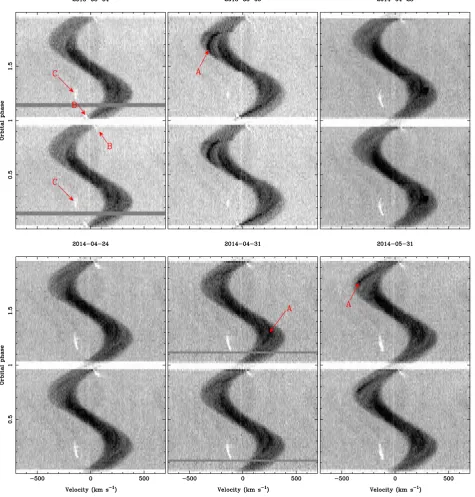
In addition to emission from the M star, there is also a narrow absorption line moving in antiphase to the M star, but only visible at certain orbital phases. This absorption is seen just before and after the eclipse of the white dwarf (labelled ‘B’ in Fig.2, particularly clear in the 2013 data) as well as close to phase 0.25, labelled ‘C’. When visible, these absorption features have the same velocity as the white dwarf (see Section 3.3), implying that this material blocking the light of the white dwarf has no radial velocity relative to it, and suggests that it is in a state of solid-body rotation with respect to the binary, likely in the form of prominences.
The most striking aspect of Fig.2is that these prominence fea-tures appear to persist on time-scales of days, weeks, months and years. Given the similarity of the prominence feature detected at on orbital phase of 0.16 in the 2002 spectra by Parsons et al. (2011), it also appears that these features could be stable on time-scales of decades. However, Fig.2also shows that they are not completely fixed. The absorption feature around phase 0.25 is visible for longer period during 2014 compared to the 2013 data. Meanwhile the ab-sorption around the eclipse is much clearer in the 2013 data and is only obvious before the eclipse in the 2014 data set.
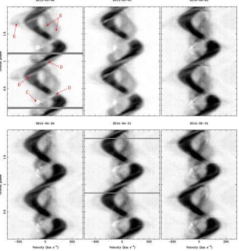
In Fig.3, we show the same plots as Fig.2but for the Hαline. This line shows a much more complex behaviour, with multiple absorption and emission components visible. The strongest com-ponent is still the emission from the M star, but narrow absorption components are seen crossing this emission throughout the orbit during all six observations (the strongest are labelled ‘D’ in Fig.3). The prominence material passing in front of the white dwarf is still visible (‘C’), albeit slightly weaker than in the CaIIline since
the white dwarf contributes a smaller amount of the overall flux at Hα. Furthermore, there are several additional emission components which do not correspond to either star in the binary, labelled ‘E’. The Hαline also shows considerable variability in the strength of all these features from night-to-night compared to the CaIIline.
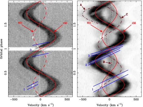
In Fig.4, we show a larger version of the CaIIand Hαtrailed spectrogram from the second observing run (2015 May 5) with some of the major features labelled. The radial velocity of the white dwarf and M star are shown as red lines (see Sections 3.3 and 3.4). We highlight in blue three clear prominence-like absorption features visible in all six observations, that appear to cross one or both of the stars. In addition, we highlight three additional emission components visible in the Hαtrail that do not originate from either star.
To further highlight the various emission components visible in the trailed spectrogram of the Hαline, we used Doppler tomogra-phy (Marsh & Horne1988). We used theMODMAPcode described in
Steeghs (2003) to reconstruct the Doppler map shown in Fig.5, us-ing all the data from 2013 May 5. It clearly shows that the strongest
at University of Warwick on October 24, 2016
http://mnras.oxfordjournals.org/
Figure 2. Phase-folded trailed spectrograms of the CaII3934 Å line, data shown twice for visual continuity. The date at the start of the night the data were obtained is shown above each plot. Higher fluxes are darker. The main features visible are the emission from the active M star and the eclipse of the white dwarf. However, a narrow absorption feature is visible just before and after the eclipse (‘B’) and at phase 0.25 (‘C’) in all the plots. This is caused by material moving in front of the white dwarf and, although variable, is always visible, despite the data spanning more than a year.
emission component originates from the M star itself, but the three additional emission components visible in the trailed spectrogram are seen more clearly, with two close to the white dwarf’s Roche lobe and one high-velocity emission component. These components are labelled ‘A’, ‘B’ and ‘C’ and correspond to the additional emis-sion seen in the Hαtrail in Fig.4, where we have used the same labels to highlight the features.
The clearest prominence feature in Fig.4, labelled ‘1’, is respon-sible for the narrow absorption line seen at around phase 0.25 in the CaIIline, when it passes in front of the white dwarf. At around
phase 0.4 this same material passes in front of the M star, completely blocking the Hαemission component from this star. Furthermore, this prominence is seen in emission at certain orbital phases, high-lighted as component ‘C’ in both Figs4and5. It is possible that the prominence is dense enough that it is able to reprocess the light it receives from the white dwarf. Alternatively, this could be intrinsic emission from the prominence. Fig.3shows that the strength of this emission clearly varied from 2013 to 2014, weakening in 2014.
The fact that this prominence crosses in front of both stars al-lows us to triangulate its position within the binary. Fig.6shows a
at University of Warwick on October 24, 2016
http://mnras.oxfordjournals.org/
Figure 3. Phase-folded trailed spectrograms of the Hαline, data shown twice for visual continuity. The continuum has been subtracted from each spectrum and on the date at the start of the night, the data obtained is shown above each plot. Higher fluxes are darker. The strongest component is emission from the active M star. However, there are at least two other emission components (‘E’), neither of which originate from either of the stars. Material is seen moving across the face of both the white dwarf (‘C’) and M star (‘D’). Despite being separated by more than a year, the trails look remarkably similar.
visualization of the binary indicating both the location and size of this prominence. We show this for both 2013 and 2014, variations on shorter time-scales are minimal. As is evident from Figs2and3, the prominence is larger in 2014, clearly taking longer to pass in front of the white dwarf. We also show the viewing angle to the white dwarf in the 2002 data from Parsons et al. (2011) which also passed through a similar prominence feature.
The stability and longevity of this feature is remarkable, given that it is located at an unstable location within the binary and hence the material should be expelled quickly. In Fig.6, we plot the
effective ‘co-rotation’ radius of the binary. While this radius is well defined for a single star (the radius at which the gravitational attraction equals the centripetal acceleration of a particle in solid-body rotation with the star, hence a particle can sit there with no other force needed to hold it), such a radius does not exist for a binary. In this case, the centripetal acceleration acts towards the centre of mass, but the gravitational forces act towards the two stars and so there is not a stable radius, but rather five equilibrium points (the Lagrangian points). However, in Fig.6, we slightly extend the definition by considering the radial component of acceleration in
at University of Warwick on October 24, 2016
http://mnras.oxfordjournals.org/
Figure 4. Trailed spectrogram of the CaII3934 Å (left) and Hα(right) lines from 2015 May 5 with the main features labelled. The velocities of the two stars
are indicated by the bright red sinusoids. In blue, we highlight three clear absorption features that cross one of both of the stars (only two are visible in the CaII
trail). We also highlight three other emission components in the Hαtrail with dark red lines.
the rotating frame (automatically including gravity and centripetal terms) as measured from the centre of mass of the M star, resulting in a line that passes through the Lagrangian points. Nevertheless, except for at the Lagrangian points themselves, there are still forces acting perpendicular to this line, so it does not represent a stable region within the binary, hence some additional force is required to keep material in this region. However, it may well be easier for material to stay fixed near this line than at other locations. From Fig.6, it is evident that material is located at this radius, but also extends substantially beyond it, requiring that quite significant non-gravitational forces are acting upon it (presumably some sort of magnetic force).
The feature labelled ‘2’ in Fig.4crosses the M star at an or-bital phase of ∼0.75, but does not appear to pass in front of the white dwarf (hence it is not visible in the CaIItrail), meaning that we cannot completely determine its location or size like the large prominence. It is possible that it passes in front of the white dwarf shortly before or during the eclipse, in which case, it would be located close to the surface of the M star. Or instead, this particu-lar prominence could be at an inclination such that it only passes in front of the M star. This prominence weakened considerably be-tween 2013 and 2014 and is barely visible in the last observations in Fig.3. There does not appear to be an obvious emission component associated with this prominence.
The feature labelled ‘3’ in Fig.4crosses the face of the M star during the eclipse of the white dwarf, and therefore this material must be located behind the M star, from the white dwarf’s perspec-tive. Moreover, the CaIItrail shows that this material also passes
in front of the white dwarf just before and after the eclipse. Un-fortunately, this means that we cannot determine the exact location of this material either. This prominence is seen in emission as a high-velocity component blueward of the M star at phase 0.75 (la-belled ‘A’) in the Hαtrail (dot–dashed line) and more clearly at (−650,450) in Fig.5. Similar absorption features were detected in ultraviolet spectra of V471 Tau just before and after the eclipse of the white dwarf (Guinan et al.1986), which they attributed to cool coronal loops. Interestingly, O’Donoghue et al. (2003) detected a sharp pre-eclipse dip in the light curve of QS Vir (see their fig. 8) which could be from similar coronal loops, implying that this ma-terial can sometimes be dense enough to block out continuum light. However, the lack of a comparison star during this observation means that this dip should be interpreted with some caution. De-spite our extensive photometric monitoring (e.g. Table1), this dip has not been seen since.
Finally, there is another emission component highlighted in the Hα trail in Fig. 4 by a dotted line (labelled ‘B’). It moves in antiphase with the M star, but with a much lower velocity than the white dwarf, meaning that this must originate from material
at University of Warwick on October 24, 2016
http://mnras.oxfordjournals.org/
Figure 5. Doppler map of the Hαline from 2013 May 5. The Roche lobes of the white dwarf and M star are highlighted with a black dashed line and solid white line, respectively. To highlight the additional emission features against the strong emission from the M star, we have also plotted contours. Three clear emission features that do not originate from either star are labelled.
between the two stars. It is also visible in Fig.5close to (0,0), within the Roche lobe of the white dwarf. Fig.3shows that this emission was much stronger in 2014 compared to 2013. Assuming that this material co-rotates with the binary, its location is given by
Kmat
Ksec
=(1+q)
R a
−q, (1)
whereKmatandKsecare the radial velocity semi-amplitudes of the
material and the M star, respectively,qis the mass ratio andR/a
is the distance of the material from the white dwarf scaled by the orbital separation (a).
Using our measured values ofKsecandq(see Sections 4 and 5) and Kmat= −100 km s−1determined by Gaussian fitting in the same way
as outlined in the next section, givesR/a=0.09. Similar emission features have been seen in other PCEBs (Tappert et al.2011; Parsons et al.2013b) as well as cataclysmic variables (CVs; Steeghs et al. 1996; G¨ansicke et al.1998; Kafka et al.2005; Kafka, Honeycutt & Howell2006) and could be related to another prominence structure or heated material from the wind of the M star close to the white dwarf. Interestingly, there appears to be a genuine deficiency of Hαemission from the inner face of the M star, best seen in Fig.5. The deficiency may be due to this material between the two stars shielding the M star from irradiation by the white dwarf.
[image:8.595.49.287.56.290.2]Despite being an eclipsing system, the inclination of QS Vir is relatively low (i= 77.7◦, see Section 5), therefore, not only are these prominences far from the M star, they are also located far from its equatorial plane. However, many cool, isolated low-mass stars show similar prominence systems beyond their co-rotation radii (Donati et al.1999; Dunstone et al.2006), and located far from their equatorial planes (Collier Cameron & Robinson1989). Indeed, Jardine et al. (2001) found that for single stars, there exist stable locations both inside and outside the co-rotation radius and up to 5 stellar radii from the star (Jardine & van Ballegooijen2005).
Figure 6. A top-down view of the binary indicating the location of the large
prominence feature in 2013 and 2014 (feature ‘1’ in Fig.4), the stars rotate
clockwise and the viewing angle to the white dwarf at various orbital phases is shown in blue. The dotted lines indicate the Roche lobes of the two stars, the radius of the M star is shown as a solid line. The arrow indicates the viewing angle to the white dwarf during the 2002 observation from Parsons
et al. (2011) in which prominence material was also observed. The cross
marks the location of the white dwarf and the black points indicate the location of the five Lagrange points. The outer solid black line indicates the effective ‘co-rotation’ radius of the binary (see the text for a definition of this radius).
Long-lived prominences have also been detected in the CVs BV Cen (Watson et al.2007), IP Peg and SS Cyg (Steeghs et al.1996) and AM Her (G¨ansicke et al.1998). Magnetically confined material was also detected in BB Dor (Schmidtobreick et al.2012) and near the L4 and L5 Lagrange points in AM Her (Kafka et al.2008). In addition, the detached white dwarf plus main-sequence star binaries V471 Tau (Jensen et al.1986) and SDSS J1021+1744 (Irawati et al.2016) both show long-lived prominence-like features, in very similar positions to the large prominence in QS Vir.
3.3 White dwarf radial velocity amplitude
We measure the radial velocity amplitude of the white dwarf using the narrow MgII4481 Å absorption line. Due to emission from the
M star, the cores of the hydrogen Balmer lines are not visible, thus making them unsuitable for radial velocity work. No other intrinsic white dwarf absorption features are detected in the UVES spectra.
We fit the MgIIline in each spectrum with a combination of a
straight line and a Gaussian component. We do not fit the spec-tra obtained whilst the white dwarf was in eclipse (including the ingress and egress phases). Furthermore, we do not fit the spec-tra taken during phases 0.45–0.55, since during these phases MgII
emission from the heated inner hemisphere of the M star fills in the absorption as the two components cross over. The resultant
at University of Warwick on October 24, 2016
http://mnras.oxfordjournals.org/
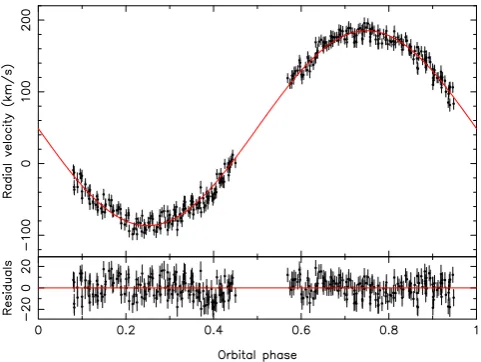
Figure 7. Radial velocity measurements of the MgII4481 Å absorption line from the white dwarf with fit (red line). The residuals of the fit are shown in the bottom panel.
velocity measurements and their corresponding orbital phases were then fitted with a sinusoid to determine the white dwarf’s radial velocity semi-amplitude. The result of this is shown in Fig.7. We find a radial velocity semi-amplitude for the white dwarf of 139.0
± 1.0 km s−1, with a mean velocity of 43.2 ± 0.8 km s−1,
con-sistent with (but much more precise than) the measurement from O’Donoghue et al. (2003) (137±10 and 61±10 km s−1,
respec-tively) usingHubble Space Telescope(HST) spectra, although our mean velocity is a little lower than their measured value. The mean velocity of the white dwarf is redshifted from the systemic velocity of the binary due to its high gravity, which can be used to constrain its physical parameters (see Section 5).
3.4 M star radial velocity amplitude
We attempted to measure the radial velocity semi-amplitude of the M star using the same technique outlined in the last section (i.e. a Gaussian fit) and fitting the NaI8200 Å absorption doublet. Fig.8 shows the result of this fit. At first glance, it seems that the semi-amplitude is tightly constrained by the data (the average uncertainty on an individual velocity measurement is∼1 km s−1). However, as
the residuals show, the deviation from a pure sinusoid are quite pronounced and there are clearly large systematic trends affecting the velocity measurements. These deviations are seen in the data from both 2013 and 2014 as well as for other atomic features, such as the KI7665 and 7699 Å lines. Therefore, we do not consider these
measurements a true representation of the centre-of-mass velocity of the M star.
The most likely cause of this deviation is the presence of starspots on the surface of the M star, although gravity darkening and irradi-ation may also contribute to this. Therefore, in order to determine a more reliable value for the radial velocity semi-amplitude for the M star, as well as a better understanding of the starspot distribu-tion and evoludistribu-tion, we used our UVES spectra to perform Roche tomography of the M star, which we detail in the following section.
4 R O C H E T O M O G R A P H Y
[image:9.595.43.284.56.237.2]Roche tomography is a technique analogous to Doppler imaging (e.g. Vogt & Penrod1983), and has been successfully used to image surface features on the secondary stars in interacting binaries. The
Figure 8. Radial velocity measurements of the NaI8200 Å absorption doublet from the M star using a Gaussian fit from the 2013 observations. The red line in the top panel is the centre-of-mass radial velocity of the M star determined from our Roche tomography analysis (see Section 4). Clear deviations from this fit are seen in the residuals in the lower panel as a result of the large number of starspots. The red line in the lower panel shows the deviations from the centre-of-light to the centre-of-mass radial velocity as determined from our Roche tomography analysis of the 2013 data, and show a very similar behaviour to the Gaussian measurements.
technique assumes the secondary star rotates synchronously in a circular orbit around the centre of mass, and uses phase-resolved spectral line profiles to map the line-intensity distribution across the star’s surface in real space. The method has been extensively ap-plied to the secondary stars in CVs over the last 20 years (Rutten & Dhillon1994,1996; Watson et al.2003; Schwope et al.2004; Wat-son, Dhillon & Shahbaz2006; Watson et al.2007; Hill et al.2014), and artefacts arising from systematic errors are well character-ized and understood. For a detailed description of the methodology and axioms of Roche tomography, we refer the reader to the refer-ences above and the technical reviews by Watson & Dhillon (2001) and Dhillon & Watson (2001).
4.1 Least squares deconvolution
Spot features appear in absorption line profiles as an emission bump (actually a lack of absorption), and are typically a few per cent of the line depth. Thus, very high SNR data are required for surface imaging, a feat not directly achievable for a single absorption line with QS Vir due to its faintness and the requirements for short ex-posures to avoid orbital smearing. To greatly improve our SNR, we employ least squares deconvolution (LSD), a technique that stacks the thousands of stellar absorption lines observable in a spectrum to produce a single ‘mean’ profile. First applied by Donati et al. (1997), the technique has been widely used since (e.g. Barnes et al. 2004; Shahbaz & Watson2007). For a more detailed description of LSD, we refer the reader to the above references as well as the review by Collier Cameron (2001).
To generate the LSD line profiles, the continuum must be flat-tened. However, the contribution of the M star to the total system luminosity may vary due to variations in accretion luminosity (see Section 6.3), and the rapid flaring on the M star on time-scales of several minutes (O’Donoghue et al.2003). Both of these mecha-nisms may change the continuum slope, and so a master continuum fit to the data is not appropriate. Furthermore, normalization of the
at University of Warwick on October 24, 2016
http://mnras.oxfordjournals.org/
46 absorption lines were used, lying in the spectral ranges 8400– 8470 Å and 8585–8935 Å. As QS Vir is an eclipsing binary, there are significant features in the line profiles arising between phases 0.4 and 0.6 (superior conjunction) which do not originate on the secondary. As inclusion of these phases would cause artefacts to appear on the reconstructed maps (e.g. the entire inner hemisphere would appear to be irradiated), they were excluded from the fitting process. The LSD profiles were then binned on a uniform velocity scale of 7.4 km s−1to match the velocity smearing due to the orbital
motion.
The LSD profiles exhibited a clear continuum slope that was largely removed by subtracting a second-order polynomial fit to the continuum, preserving the profiles’ features and shape. However, these corrected profiles still exhibited a non-flat continuum which lay significantly below zero. To account for this, a constant offset was added to each set of LSD profiles, the specific value of which was non-trivial to determine due to degeneracies in the fitting pro-cess; if a small constant was added, a greater proportion of the line wings lay below the continuum, inflating the Roche lobe and chang-ing the optimum masses found in the fit with Roche tomography. If a large constant was added, more of the line wings lay above the continuum, changing the optimum system parameters. Hence, an optimum value of constant to add to the LSD profiles could not be found computationally. Instead, the most appropriate offset was found by visual inspection of the fits to the data. This was done in-dependently for each data set. These offset and continuum-flattened LSD profiles were then adopted for the rest of the fitting process with Roche tomography.
In general, Roche tomography cannot normally be performed on data which has not been corrected for slit losses, due to the secondary star’s variable light contribution. As the acquired data of QS Vir was largely photometric, we were able to correct for slit losses using an optimal-subtraction technique. Here, each LSD profile was scaled and subtracted from the fit made with Roche tomography, where the optimal scaling factor was that which minimized the residuals. The newly scaled LSD profiles were then re-fit with Roche tomography, and the above process repeated until the scaling factors no longer varied. The resulting scaled profiles were visually inspected and found to be consistent. The final LSD profiles with computed fits and residuals are shown in Fig.9.
4.2 System parameters
Roche tomography constrains the binary parameters by reconstruct-ing intensity maps of the stellar surface for many combinations of
M1,M2, inclination (i), systemic velocity (γ) and Roche lobe filling
factor (RLFF). Each map is fit to the sameχ2. However, for a given
(Parsons et al. 2011). Additionally, the inclination was fixed to
i= 77◦.8, as this was well constrained from light-curve analysis – considering the SNR of the data being fit, we are unlikely to improve the accuracy of this using Roche tomography, and indeed an unsuccessful attempt was made to constrain inclination once optimal system parameters were found.
4.2.1 Limb darkening
Roche tomography allows limb darkening to be included in the fit-ting of line profiles. In order to calculate the correct limb darkening coefficients, we determined the effective central wavelength of the data over ranges specified in Section 4.1 using
λcen=
i
1
σ2
i diλi
i
1
σ2
i di
, (2)
wheredi is the line depth at wavelengthλi, andσi the error in the data atλi. The mean value ofλcenacross the six data sets was
used for consistency. We adopted a four-parameter non-linear limb darkening model (see Claret & Bloemen2011), given by
I(μ)
I(1) =1−
4
k=1
ak(1−μ
k
2), (3)
whereμ=cosγ(γ is the angle between the line of sight and the emergent flux), andI(1) is the monochromatic specific intensity at the centre of the stellar disc.
Using the calculatedλcen, the limb darkening coefficients were
then determined by linearly interpolating between the tabulated wavelengths given in Claret & Bloemen (2011). We adopted stellar parameters closest to that of a M3.5V star, which for the PHOENIX model atmosphere were logg=5 and Teff = 3100 K. Thus, the
adopted coefficients werea1=3.302,a2= −5.057,a3=4.612, a4= −1.61. We note that the limb darkening law used is for
spheri-cal stars, and so is not ideally suited to the distorted main-sequence star in QS Vir. Ideally, one would need to calculate limb darkening coefficients for each tile in the grid based on a model atmosphere. However, this is not currently possible within our code, and so we adopted uniform limb darkening coefficients. Artefacts arising from adopting incorrect coefficients are discussed in Watson & Dhillon (2001).
4.2.2 Systemic velocity
The entropy statistic is most sensitive to an incorrect systemic veloc-ityγ, and so this parameter was narrowed down most easily. Fig.10
at University of Warwick on October 24, 2016
http://mnras.oxfordjournals.org/
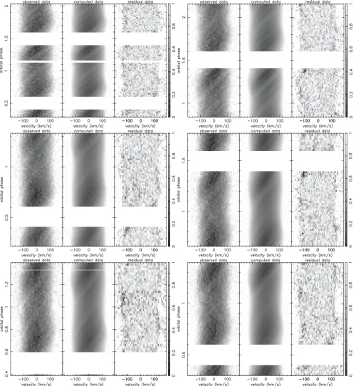
Figure 9. Trailed LSD profiles of QS Vir (2013-05-04 top left, 2013-05-05 top right, 2014-04-23 middle left, 2014-04-24 middle right, 2014-04-31 bottom left, 2014-05-31 bottom right). From left to right, panels show the observed LSD data, computed data from the Roche tomography reconstruction and the residuals (increased by a factor of 4). Starspot features in these panels appear bright. A grey-scale wedge is also shown, where a value of 0 corresponds to the maximum line depth in the reconstructed profiles. The orbital motion has been removed assuming the binary parameters found in Section 4.2, which allows
the individual starspot tracks across the profiles and the variation inVrotsinito be more clearly observed.
shows the map entropy yielded for each data set as a function ofγ, where a cross marks theγthat gives the map of maximum entropy. The mean value across all data sets yieldsγmean= −4.4+−00..59km s−1,
where the uncertainties represent the spread between maximum and minimum for all measured values. We also determined the radial
velocity semi-amplitude of the M star as 275.8±2.0 km s−1. Note
that the radial velocity semi-amplitude of the M star is calculated from the resulting stellar parameters (masses, inclination etc.) rather than being a direct input to the fit. As mentioned in Section 3.4, we consider these values more reliable than those from Gaussian fitting,
at University of Warwick on October 24, 2016
http://mnras.oxfordjournals.org/
Figure 10. Points show the maximum entropy value obtained in each data set, as a function of systemic velocity. The optimal masses and RLFF as found in Section 4.2.3 were adopted for the fits of each data set. The points are plotted with a vertical offset of 0.1 between data sets. Crosses mark
the value ofγthat yields the map of maximum entropy, and a sixth-order
polynomial fit is shown as a visual aid. The mean systemic velocity across
all data isγmean= −4.4+0−0..59kms−
1.
due to the surface inhomogeneities biasing those results and indeed once these surface features are taken into account, the measured velocities match the reconstructed model from Roche tomography (see the lower panel of Fig.8).
4.2.3 RLFF and masses
Readers should note that, unless otherwise stated, the value of the RLFF is given as the ratio of the volume averaged radius of the M star to its Roche lobe radius, as opposed to the linear RLFF which is given by the distance from the centre of mass of the M star to its surface in the direction of the L1 point divided by the distance to the L1 point.
Fig. 11 shows the map entropy as a function of RLFF. For a given RLFF, the optimal masses are determined by reconstructing maps for many pairs of component masses. The optimalM1and M2are those that produce the map of maximum entropy (an
‘en-tropy landscape’, see fig. 8 of Hill et al.2014). The values ofγ
[image:12.595.310.551.57.343.2]determined in Section 4.2.2 were adopted for the fits, and recon-structions were performed in steps of 0.5 per cent for the RLFF, and in steps of 0.1 Mfor the masses. The points follow a roughly parabolic trend with some small ‘jumps’ in entropy that are mainly due to the change in grid geometry, due to varying masses and RLFF, combined with rounding errors in the code. However, all optimum RLFFs determined from each independent data set are in close agreement, ranging between 96 and 98 per cent, and so we can be confident that the measured RLFF and masses are robust.
Figure 11. Points show the map entropy obtained in each data set as a function of RLFF, where optimal masses were used for each RLFF. The optimal systemic velocities found in Section 4.2.2 were adopted for the map reconstructions. The points are plotted with a vertical offset of 0.1 between data sets. Crosses mark the maps of maximum entropy, yielding the optimal masses at the optimal RLFF. Fourth-order polynomial fits are shown as a visual aid. The peaks of these fits were not used to determine the optimal RLFF, as the high-order nature of the polynomial meant the fits were often
skewed. The mean RLFF across all data is 97±1 per cent, where the
uncertainty represents the spread between maximum and minimum for all measured values.
The amount of scatter in the entropy ‘parabolas’ is consistent with the low SNR of the data being fit – similar scatter was found when performing Roche tomography with relatively low-quality data of the CVs AM Her and QQ Vul (Watson et al.2003).
There are a number of possible sources of systematic error when fitting data of poor SNR with Roche tomography. In this instance, the dominant source of uncertainty in the system parameters is due to the difficulty in determining the true continuum level of the LSD profiles, as discussed in Section 4.1. If the continuum is too low, the Roche lobe is artificially inflated to fit the line wings, resulting in larger measured masses. Furthermore, if the continuum is set too high, the Roche lobe is artificially underfilled. To determine the impact of choosing an incorrect continuum level, a range of offsets were added to the LSD profiles, and for each offset, the LSD profiles were fit and scaled as described in Section 4.1. The optimal masses found for each offset were then compared and, across all data, the maximum difference between the optimal primary and secondary masses were 3.8 per cent and 7.9 per cent, respectively, and the spread in RLFF was 1 per cent. Hence, while only a visual check was made of the fits to the continuum level of each set of LSD profiles, the optimal masses and RLFF found for each data set agree within these uncertainties.
at University of Warwick on October 24, 2016
http://mnras.oxfordjournals.org/
Figure 12. Trailed LSD profiles of QS Vir using phase-binned data from all data sets. A mean of the computed LSD profiles has been subtracted from both the observed and computed LSD profiles. Starspot features in these panels appear dark. The orbital motion has been removed assuming the binary parameters found in Section 4.2.
The mean RLFF is 97±1 per cent, with the mean of the masses yielding MWD=0.76−+00..0201M and MdM=0.358+−00..022018M,
re-spectively, where all uncertainties represent the spread between the maximum and minimum values. Hence, the mean mass-ratio was found to beq=0.47± 0.04. In Section 5 we will combine the spectroscopic constraints with our light-curve data to determine more precise values for these parameters, but quote these Roche tomography values here for completeness. Using the mean sys-tem parameters with our model grid, we calculatevsinito range between a minimum of 117.8 km s−1at phase 0 and 0.5, to a
maxi-mum of 133.5 km s−1at phase 0.25 and 0.75. Our measured masses
and RLFF agree well across all data sets, and so for consistency in comparing maps, we adopted the mean values for the final map reconstructions (see Fig.13).
4.3 Surface maps
The mean system parameters found in Section 4.2 were used to construct Roche tomograms of all data sets. The corresponding trails of LSD profiles are displayed in Fig.9. Evident in both the trails and the maps are numerous spot features, with three large-scale features common to all trails and maps (marked A, B and C in Figs12and13). The technique of Roche tomography is shown to be remarkably robust in the reconstruction of these features – maps reconstructed independently with data taken on sequential nights show very similar features. The morphologies of these three features remain fairly unchanged over the 1 yr period of observations, with no apparent movement across the stellar surface, indicating that these are indeed long-lived starspots. Furthermore, smaller scale structure is apparent in both the data and fits from the 2013 data, however, the same level of detail is not as readily reconstructed using other data sets, most likely due to the fewer number of LSD profiles being fit.
[image:13.595.44.283.58.249.2]There is a distinct lack of a large high-latitude spot. Such a feature is commonly seen on Doppler imaging studies of rapidly rotating single stars (e.g. Donati et al.1999; Hussain et al.2007), and in CVs such as BV Cen and AE Aqr (Watson et al. 2006; Watson et al.2007). Given the presence of such a feature in these
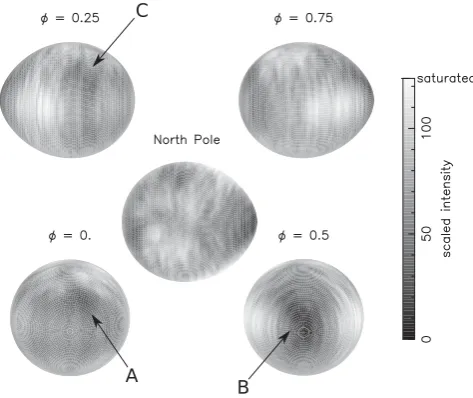
Figure 13. Roche tomogram of QS Vir using phase-binned data from all data sets. Dark grey scales indicate regions of reduced absorption line strength that is due to either the presence of starspots or the impact of irradiation. The contrast in these Roche tomograms has been enhanced such that the darkest and lightest grey scales correspond to the lowest and highest intensities in the reconstructed map. The orbital phase is indicated above each panel, and Roche tomograms are shown without limb darkening for clarity.
other rapidly rotating stars, it is surprising to find that a large high-latitude spot does not exist here. Pertinently, a study by Morin et al. (2008) finds that large-scale, mainly axisymmetric poloidal fields are fairly common in fully convective M dwarfs, observing polar region spots on three out of the six stars in their sample. However, the authors also found that the partly convective star AD Leo hosted a similar magnetic field, but with significantly lower magnetic flux, indicating the generation of large-scale magnetic fields is more efficient in fully convective stars. As the measured mass of the M dwarf in QS Vir suggests it has a partly radiative core, the lower efficiency of magnetic field generation may mean any polar region spots are significantly less obvious.
Alternatively, the lack of a large high-latitude feature may simply be due observational effects – given the inclination ofi=77.8◦ in QS Vir, high latitudes appear severely foreshortened, and are heavily limb-darkened. These effects, combined with the poor SNR of the data, may mean high-latitude features are simply lost in the noise. This was assumed to be the case by Barnes & Collier Cameron (2001) who found a similar lack of polar spot features in their study of HK Aqr (i=70◦–90◦), with simulations showing that reconstructions of high-latitude features strongly depend on the SNR of the data.
Other prominent features on the maps are the dark regions around the L1point, marked ‘B’ in Figs12and13. In previous maps of
CVs (e.g. Watson et al.2003), features on this part of the star were attributed to irradiation effects from the white dwarf, where ion-ization of the photosphere causes a decrease in photometric flux. However, the features reconstructed here are patchy in morphology, rather than smoothly varying, which suggests that irradiation is not the main contributing factor of the features in this region. This was tested by simulating a realistic irradiation pattern, and fitting the data using the same phases as that of the phase-binned LSD profiles shown in Fig.12. The reconstructed irradiation pattern was found to be smoothly varying, and was essentially uniform around the
at University of Warwick on October 24, 2016
http://mnras.oxfordjournals.org/
Tau (Hussain et al.2006), the eclipsing binary ER Vul (Xiang et al. 2015), and the close binaryσ2CrB (Strassmeier & Rice 2003).
Furthermore, Kriskovics et al. (2013) suggested that the hotspots mapped on the companion-facing hemisphere in V824 Ara may indicate the strong interaction between the magnetic fields of the component stars, as is commonly observed in close RS CVn-type binaries. This phenomenon was discussed in Hill et al. (2014), where spot ‘chains’ from the pole to L1point (on multiple CVs) suggested a
mechanism that forces magnetic flux tubes to preferentially emerge at these locations. Indeed, Holzwarth & Sch¨ussler (2003) propose that tidal forces may cause spots to form at preferred longitudes, and Moss, Piskunov & Sokoloff (2002) suggest that this phenomena may also be due to the tidal enhancement of the dynamo action itself.
Other features of interest include a prominent starspot labelled ‘A’ in Fig.13. It stretches∼5◦–25◦in longitude, and∼15◦–35◦in latitude (where the back of the star is at 0◦longitude, with increasing longitude in the direction of the leading hemisphere). Finally, label ‘C’ in Fig.13points to a group of spots covering 275◦–300◦ lon-gitude and spanning 20◦–55◦latitude. Given that the phase-binned data has a longitudinal resolution of∼6◦, we can reliably separate the larger spots in this group – one spot extends 275◦–285◦ lon-gitudinally and 35◦–55◦in latitude, and another spans 293◦–300◦ in longitude and 15◦–30◦latitudinally. As both ‘A’ and ‘C’ can be seen in all data trails taken over a∼1 yr period, they are most likely groups of long-lived starspots.
The prominent spotted regions labelled ‘A’ and ‘B’ (located at phasesφ∼0.05 and 0.5, respectively) are similar to those found by Ribeiro et al. (2010) in their maps of QS Vir made using photometry taken in 1993 and 2002. The authors find two cool regions atφ∼0.4 and 0.9 that show little shift in longitude between 1993 and 2002. The authors’ photometric data does not allow for a tight constraint on latitude, however, if these spotted regions are the same as those imaged here (namely features ‘A’ and ‘B’), they may be very long lived active regions that have remained at the same longitudes for over 20 years.
4.3.1 Spot coverage as a function of longitude and latitude
[image:14.595.309.549.58.246.2]To make a more quantitive estimate of spot parameters on QS Vir, we have examined the pixel intensity distribution in the Roche tomogram. By visual inspection, all reconstructed maps appeared to have a very similar distribution of spots, with small-scale variation due to differences in SNR and number of spectra between data sets. For an improved estimate of spot coverage, we combined all data sets by phase-binning the LSD profiles over 60 evenly spaced phase
Figure 14. Fractional spot coverage as a function of latitude, normalized by the surface area of that latitude, as calculated for the reconstructed map using phase-binned data. The geometry the grid in our Roche tomogram does not allow for strips of constant latitude, and so we are required to interpolate between grid elements. We have done this by taking a moving-mean with a
5◦window in steps of 1◦.
bins (each containing∼7 LSD profiles). We only present analysis of the map that was reconstructed using this binned data (see Fig.13). The high inclination of the system causes a ‘mirroring’ effect, as described in section 3.11 of Watson & Dhillon (2001). As ra-dial velocities cannot constrain whether a feature is located in the Northern or Southern hemisphere, features are mirrored about the equator. This means features become less apparent due to the fact that they are first latitudinally smeared, and then mirrored, caus-ing the streaks seen in the maps presented here. To mitigate this effect, we discarded all pixels in the Southern hemisphere for the remainder of this analysis.
Each pixel in our Roche tomograms was given a spot filling-factor between 0 (immaculate) and 1 (totally spotted). The value for any given pixel depended on its intensity, and was scaled lin-early between our predefined immaculate and spotted photosphere intensities. It is unlikely that the highest intensities represent the immaculate photosphere, as the growth of bright pixels in maps that are not ‘threshholded’ is a known artefact of Doppler imaging techniques (e.g. Hatzes & Vogt1992). Instead, we have defined an intensity of 92 and above to represent the immaculate photosphere. Furthermore, we have defined a 100 per cent spotted pixel by taking the minimum pixel intensity in the group of spots marked ‘B’ in Fig.13, avoiding the very front pixels on the model star as these may be additionally affected by gravity darkening or irradiation.
Based on our classification of a spot, we estimate that 35 per cent of the Northern hemisphere of QS Vir is spotted. This is likely to be a lower limit due to the presence of unresolved spots – O’Neal, Neff & Saar (1998) estimated up to 50 per cent fractional spot coverage in TiO studies of rapidly rotating G- and K-type stars, and Senavci et al. (2015) find a factor∼10 difference between spot filling factors when comparing TiO analysis to Doppler imaging. Furthermore, Hessman, G¨ansicke & Mattei (2000) predict a mean spot coverage of∼50 per cent on the CV, AM Her, using long-term light-curve analysis.
When plotted as a function of latitude (see Fig.14), we see a clear increase in fractional spot coverage at low to mid-latitudes (10◦–50◦) of around 0.2, as compared to the spot coverage at higher
at University of Warwick on October 24, 2016
http://mnras.oxfordjournals.org/
Figure 15. Fractional spot coverage as a function of longitude, as calculated for the reconstructed map using phase-binned data. Points are calculated by
taking a moving-mean with a 6◦window (the longitudinal resolution of the
map), in steps of 1◦.
latitudes (50◦–90◦). This large spread in latitude may be indicative of a distributed dynamo, with many unresolved small-scale fea-tures spread across the stellar surface. A more likely explanation, however, is that the spread is due to features becoming smeared in latitude due to both poor SNR, and from limitations in the technique (as discussed above). Also apparent is a small increase in spot cov-erage at high latitudes (centred∼74◦). As discussed above, the spot contrast at higher latitudes is diminished in this system due to is high inclination, and so the measured spot coverage is likely underesti-mated at these latitudes. Similar distributions of spots were found on the M dwarfs HK Aqr and RE 1816+541 by Barnes & Collier Cameron (2001), with the majority of features equally distributed over 20◦–80◦latitude.
When plotted as a function of longitude in Fig.15, we find a large increase in fractional spot coverage around 15◦, 180◦, and 285◦longitude, corresponding to the features marked A, B and C, respectively, as shown in Fig.13. As previously discussed, the large increase around 180◦is similar to that found on CVs (e.g. AE Aqr, Hill et al.2014) and on pre-CVs (e.g. V471 Tau; Hussain et al. 2006).
4.3.2 Magnetic activity and starspot lifetime
The features marked A, B and C in Figs 12 and 13 are clearly observed in all data sets from 2013 May to 2014 April, and appear to remain in fixed positions over both short and long time spans. This suggests a very low level of surface shear, with no perceivable shift over the∼1 yr between first and last observations. As the M star in QS Vir is very close to becoming fully convective, the lack of any detectable differential rotation concurs with the conclusions of Barnes et al. (2005), who found that differential rotation appears to vanish with increasing convection depth. This trend was also found in studies of rapidly rotating M dwarfs by Morin et al. (2008), where several stars in their sample exhibited fairly similar magnetic topologies over the∼1 yr period between observations. In other work, Morin et al. (2010) found both GJ 51 and WX UMa to exhibit strong, large-scale axisymmetric-poloidal and nearly dipolar fields, with very little temporal variations over the course of several years.
5 M O D E L L I N G T H E E C L I P S E L I G H T C U RV E
Eclipsing PCEBs have been used to measure precise masses and radii of both the white dwarf and main-sequence components in a number of systems (e.g. Parsons et al.2010a,2012b,c) offering some of the most precise and model-independent measurements to date for either type of star. The small size of the white dwarf leads to very sharp eclipse features, with typical ingress and egress times of around a minute or less meaning that high-speed photometry is required to properly resolve the eclipse features. With typical exposure times of<3 sec, our ULTRACAM data fully resolve the eclipse of the white dwarf and thus can be used to place stringent constraints on the physical parameters of both stars.
We model the light-curve data using a code written for the gen-eral case of binaries containing white dwarfs (see Copperwheat et al.2010for a detailed description). The programme subdivides each star into small elements with a geometry fixed by its radius as measured along the direction of centres towards the other star with allowances for Roche geometry distortion. We fitted the UL-TRACAMugrandiband light curves around the eclipse of the white dwarf. We exclude data taken at other orbital phases since the effects of starspots on the surface of the main-sequence star strongly influences the constraints that these data provide. However, the ef-fects of starspots on the white dwarf eclipse itself are minor, since it is such a rapid process. Nevertheless, starspots often lead to linear slopes across the eclipse, that vary over the time-scale of our UL-TRACAM observations. Therefore, each eclipse observation was initially fitted with a basic model using the parameters from Par-sons et al. (2010b) and including a linear slope. This slope was then removed from each light curve individually before combining them. Additionally, we shifted each eclipse in phase to remove the effects of the deviations from linearity in the eclipse arrival times.
The basic geometric parameters required to define the model are the mass ratio,q=Msec/MWD, the inclination,i, the scaled radii
of both stars,RWD/aandRsec/aand the two temperatures,Teff,WD
andTeff,sec. In addition to these, the model also requires the time of
mid-eclipse,T0, the period,Pand the limb darkening parameters
for both stars.
Since we used phase-folded data we kept the period fixed as 1, but allowedT0to vary. The temperature of the white dwarf was
fixed atTeff=14 220 K. We use the same setup for limb darkening
as detailed in equation (3) for both stars. For the M star, we use the limb darkening coefficients for aTeff=3100 K, logg=5
main-sequence star in the appropriate filter (Claret & Bloemen2011). We use the coefficients for aTeff=14 000 K, logg=8.25 white dwarf
at University of Warwick on October 24, 2016
http://mnras.oxfordjournals.org/
the longer wavelength bands where the M star dominates and hence where the white dwarf eclipse is shallower and offers poorer con-straints on its size. Therefore, this approach was not taken, although we did check that our final model results predicted an ellipsoidal modulation amplitude consistent with the ULTRACAM data. An-other method used to break the degeneracy between the inclination and scaled radii, and that we use here, is to use our measurement of the rotational broadening of the M star (Vrotsini). For a
syn-chronously rotating star this is given by
Vrotsini=Ksec(1+q)
Rsec
a , (4)
where the radial velocity semi-amplitude of the M star (Ksec) and the
mass ratio (q) have both been spectroscopically constrained. Hence, combining this with the fit to the white dwarf eclipse allows us to determine the inclination, radii of both stars and, via Kepler’s laws, the orbital separation and masses of both stars. However, as pre-viously noted in Section 4.2.3, the measured rotational broadening varies as a function of orbital phase, as the M star is not spheri-cal and hence presents a different radius at different orbital phases. Therefore, when fitting the eclipse light curve we calculated the rotational broadening of the M star at the quadrature phases (when it is at its maximum) and compared this to the maximum value determined from our Roche tomography analysis.
We used the Markov Chain Monte Carlo (MCMC) method to de-termine the distributions of our model parameters (Press et al.2007). The MCMC method involves making random jumps in the model parameters, with new models being accepted or rejected according to their probability computed as a Bayesian posterior probability. In this instance, this probability is driven by a combination of the
χ2and the prior probability from our constraints from the
spec-troscopy and Roche tomography. For each band, an initial MCMC chain was used to determine the approximate best parameter values and covariances. These were then used as the starting values for longer chains which were used to determine the final model values and their uncertainties. Several chains were run simultaneously to ensure that they converged on the same values.
This approach results in very few systematic uncertainties in the derived parameters, since the vast majority of them are directly de-termined by the data itself. The temperatures of the two stars are effectively scale factors and so have no effect. The shape of the eclipse of the white dwarf is not altered by the adopted limb dark-ening coefficients for the M star, these are mostly important for the transit of the white dwarf across the face of the M dwarf as well as any ellipsoidal modulation, neither of which we consider in our fit. However, the choice of limb darkening coefficients for the white dwarf does have some effect on the final parameters, specifically the
to night. This was taken into account by increasing the uncertainties on these two values to cover the spread of values seen on different nights. Indeed, this is the largest source of uncertainty in the fit and limits how precisely we could measure the stellar masses.
The best-fitting models to the white dwarf eclipse in theugrand
ibands are shown in Fig.16, along with their residuals. The results from all four bands were consistent and the final stellar and binary parameters are detailed in Table2. The results are consistent with those of O’Donoghue et al. (2003), but a factor of 4 more precise in mass and almost 10 in radius. In fact, the radius measurement of the white dwarf in QS Vir is the most precise, direct measurement of a white dwarf radius ever. It is remarkable that we have measured the size of an object at nearly 50 pc away to within 50 km, and highlights the potential for these kinds of systems to strongly test theoretical mass-radius relationships. The measured masses of the two stars are also consistent with the results from Roche tomography (MWD=0.76±0.01 M,MdM=0.36±0.02 M).
An additional constraint on the stellar parameters comes from the gravitational redshift of the white dwarf. For the measured pa-rameters listed in Table2, we would expect to measure a redshift for the white dwarf of 45.8±0.6 km s−1(taking into account the
redshift of the M star, the difference in transverse Doppler shifts and the potential at the M star owing to the white dwarf). Taking the difference between the systemic velocities of the two stars from our UVES data gives a measured gravitational redshift of 47.6± 1.2 km s−1, which is fully consistent with our results.
6 D I S C U S S I O N
6.1 The mass–radius relationship for white dwarfs
Fig. 17 shows the mass–radius plot for white dwarfs and high-lights the location of the white dwarf in QS Vir. We also plot the model-independent mass–radius measurements of several other white dwarfs, all members of close, eclipsing binaries. Inset we show a zoom in on the white dwarf in QS Vir compared to theoret-ical models. The measured values show excellent agreement with a carbon–oxygen core white dwarf model of the same temperature and with a thick hydrogen envelope (MH/MWD=10−4), although
the uncertainty in the measurements mean that thinner hydrogen layers cannot be ruled out. This is consistent with the results from other white dwarfs in PCEBs, such as NN Ser and GK Vir, which both possesses hydrogen envelope masses ofMH/MWD=10−4
(Par-sons et al.2010a,2012b), although several other eclipsing white dwarfs have thinner hydrogen envelopes e.g. SDSS J0138−0016 (MH/MWD =10−5; Parsons et al.2012c) and SDSS J1212−0123
(MH/MWD = 10−6; Parsons et al. 2012b). Both white dwarf
at University of Warwick on October 24, 2016
http://mnras.oxfordjournals.org/
Figure 16. Flux calibrated ULTRACAMugrandiband light curves of the eclipse of the white dwarf in QS Vir with model fits overplotted (black lines).
We have offset theiband light curve by−13 mJy to show more detail. The bottom four panels show the residuals of the fit in theuband (top panel, blue
points),gband (second panel, green points),rband (third panel, orange points) and theiband (bottom panel, red points).
components of the eclipsing binary CSS 41177 appear to have thin hydrogen layers as well (MH/MWD<10−4; Bours et al.2014).
The only other reliable white dwarf hydrogen envelope mass mea-surement in a PCEB system is for the pulsating white dwarf in SDSS J1136+0409, which was found to have an envelope mass of
MH/MWD=10−4.9(Hermes et al.2015), implying that there could
be a substantial spread in the hydrogen envelope masses of white dwarfs in PCEBs, possibly as a result of the common envelope phase itself.
The temperature and surface gravity of the white dwarf in QS Vir place it close to the blue edge of the DA white dwarf instability strip. However, our results are precise enough to firmly place it just outside the strip, which is consistent with the null detection of pulsations in our extensive high-precision photometry.
6.2 The mass–radius relationship for low-mass stars
In Fig.18, we show the mass–radius plot for low-mass (<0.5 M) stars along with a number of directly measured objects. The loca-tion of the M star in QS Vir is indicated by the contours, where we have used the volume-averaged radius. Its mass and radius mea-surements are consistent with the evolutionary models of Morales et al. (2010) for a 1 Gyr magnetically active star. Also highlighted in red are several other low-mass star mass–radius measurements from PCEB systems. The M star in QS Vir is the first low-mass star in a PCEB that is not fully convective (MdM>0.35 M) to
have high-precision, model-independent mass and radius measure-ments. While the majority of these measurements are consistent with theoretical models, two systems (SDSS J1212−0123; Parsons
et al.2012band SDSS J1210+3347; Pyrzas et al.2012) have mea-sured radii almost 10 per cent overinflated compared to these same models. Any possible explanation, for why some of these low-mass stars are overinflated, while others are not, will require more high-precision mass–radius measurements from PCEBs and more theoretical modelling of low-mass stars.
6.3 The current evolutionary state of QS Vir
The strong surface gravity of the white dwarf causes metals to sink out of the photosphere on a short time-scale. Therefore, the detection of the MgII4481 Å absorption line implies that the white
dwarf must be currently accreting some material originating from the M star. Interestingly, the strength of this absorption is variable as shown in Fig.19. It was slightly stronger in 2014 compared to 2013. This supports the idea that the accretion rate of material on to the white dwarf is variable on year time-scales and is unlikely to originate solely from the wind of the M star, but is likely driven by flare and coronal mass ejections (CME) events.
Matranga et al. (2012) detected clear X-ray eclipses, revealing that the white dwarf dominated the X-ray flux rather than the M star, supporting the idea of ongoing accretion. They determined an accretion rate of ˙M=1.7×10⁻¹³M
yr−1, which would be one
of the lowest accretion rates for a non-magnetic CV system if this were the case, but would be particularly large for a detached system. The authors speculate that a stellar wind could be the source of the observed mass transfer, invoking a magnetic ‘syphon’ model, as found by Cohen, Drake & Kashyap (2012). Matranga et al. (2012) speculated that to maintain a more constant mass supply, the wind
at University of Warwick on October 24, 2016
http://mnras.oxfordjournals.org/