warwick.ac.uk/lib-publications
Original citation:
Bove, Vincenzo and Elia, Leandro. (2016) Migration, diversity, and economic growth. World
Development.
Permanent WRAP URL:
http://wrap.warwick.ac.uk/81580
Copyright and reuse:
The Warwick Research Archive Portal (WRAP) makes this work of researchers of the
University of Warwick available open access under the following conditions.
This article is made available under the Creative Commons Attribution 4.0 International
license (CC BY 4.0) and may be reused according to the conditions of the license. For more
details see:
http://creativecommons.org/licenses/by/4.0/
A note on versions:
The version presented in WRAP is the published version, or, version of record, and may be
cited as it appears here.
Migration, Diversity, and Economic Growth
VINCENZO BOVE
aand LEANDRO ELIA
b,* aUniversity of Warwick, UK
b
European Commission – DG Joint Research Centre, Italy
Summary.—When migrants move from one country to another, they carry a new range of skills and perspectives, which nurture tech-nological innovation and stimulate economic growth. At the same time, increased heterogeneity may undermine social cohesion, create coordination, and communication barriers, and adversely affect economic development. In this article we investigate the extent to which cultural diversity affects economic growth and whether this relation depends on the level of development of a country. We use novel data on bilateral migration stocks, that is the number of people living and working outside the countries of their birth over the period 1960– 2010, and compute indices of fractionalization and polarization. In so doing, we explore the effect of immigration on development through its effect on the composition of the destination country. We find that overall both indices have a distinct positive impact on real GDP per capita and that the effect of diversity seems to be more consistent in developing countries.
Ó2016 The Author(s). Published by Elsevier Ltd. This is an open access article under the CC BY-NC-ND license (http://creativecommons. org/licenses/by-nc-nd/4.0/).
Key words— diversity, economic growth, migration
1. INTRODUCTION
The question of whether ethnic diversity affects economic performances has recently become a very active research area in a number of disciplines, including economics, development studies, management, and political science (see e.g.,Alesina & La Ferrara, 2005; Go¨ren, 2014; Horwitz & Horwitz, 2007; Posner, 2004). At the same time, research on the migration-development nexus has grown steadily, after many years of neglect, in particular within development studies (De Haan, 1999). In fact, the field has rapidly expanded in scope, emerg-ing as a proper subfield (Clemens, O¨ zden, & Rapoport, 2014). In this article we investigate the extent to which cultural diver-sity affects economic growth, using novel data on bilateral migration stocks, that is the number of people living and working outside the countries of their birth, to compute indices of heterogeneity. In so doing, we explore the effect of immigration on development through its effect on the compo-sition of the destination country.
Whether cultural diversity—the range of citizens with differ-ent origins, religions, and traditions living and interacting together—carries economic costs (e.g., Easterly & Levine, 1997) or benefits (e.g.,Ottaviano & Peri, 2006) is a highly dis-puted question among scholars.Horwitz and Horwitz (2007, p. 988) eloquently describe diversity as a ‘‘double-edged sword”. A rich pool of different expertise and experiences can potentially create organizational synergies, and hence pos-itive team outcome. Yet heterogeneous environments may also give rise to coordination problems (for instance due to lan-guage diversity or lack of trust), thus increasing transaction costs and creating irreconcilable divisions.
Our contribution to this debate is twofold. Firstly, most of the existing studies are cross-sectional and explore the effect of ethnic and linguistic diversity on economic growth using time-invariant measures based on language and ethnicity (e.g.,Alesina, Devleeschauwer, Easterly, Kurlat, & Wacziarg, 2003; Go¨ren, 2014; Montalvo & Reynal-Querol, 2005a).1This is unfortunate since the racial and ethnic composition of mod-ern societies have dramatically changed in the last few decades as a consequence of mass migration. During 1960–2000 the
global migrant stock moved from 92 million to 165 million (O¨ zden, Parsons, Schiff, & Walmsley, 2011), and continued to grow rapidly, reaching 222 million in 2010 (UNDESA., 2016). If anything, the very effect of cultural heterogeneity is likely to differ over time. Furthermore, as Horowitz (1985)
laments, interpreting ethnicity as connected only to language or race is too narrow; he instead argues that connection to birth should be the primary, if not the only, criterion. Similarly, in an interdisciplinary overview of the meaning of ethnicity and its social and political consequences, Kanbur, Rajaram, and Varshney (2011)recall how several identity categories are given to each of us at the time of birth.
Against this background, this paper uses an almost-exhaustive dataset on international migration during 1960–2010, and compute diversity by referring to a main iden-tifying characteristic, the nationality of the immigrants. The nature of the dataset coupled with our estimation technique (a variety of two-stage least-squares and panel data models) allows us to kill three birds with one stone by accounting for (i) social changes over time, (ii) cross-country variations in the starting level of development, and (iii) country-specific (time-invariant) unobservable characteristics, to avoid attribut-ing ‘‘more to diversity than is warranted”(Kanburet al., 2011, p. 150). In a similar vein, Alesina, Harnoss, and Rapoport (2016) find that diversity of skilled immigration relates positively to economic development.2 To the best of our knowledge, only a handful of studies investigate the effect of diversity on growth over time, yet they are mostly sub-national and draw on U.S. census data (e.g., Ager & Bru¨ckner, 2013; Ottaviano & Peri, 2006), thus raising concerns about the external validity of their results.
Secondly, and perhaps more importantly, the existing cross-country literature pools together low and high-income
* We are grateful to the editor, Arun Agrawal, and to three anonymous referees of this journal for their comments that have significantly improved our paper. The responsibility for any remaining errors or omissions is our own. The views here expressed are purely those of the authors and may not in any circumstances be regarded as stating an official position of the European Commission. Final revision accepted: August 13, 2016.
0305-750X/Ó2016 The Author(s). Published by Elsevier Ltd. This is an open access article under the CC BY-NC-ND license
(http://creativecommons.org/licenses/by-nc-nd/4.0/).
www.elsevier.com/locate/worlddev
countries, neglecting the possibility that diversity could play a different role at different stages of development. In fact, previ-ous estimates are unlikely to capture the complexity of the relationship because they provide an average estimate. Focus-ing on less-developed countries appears crucial in light of recently released data on migration: during 1960–2000, South-South migration dominated global trends and made up half of all international migration in 2000 (O¨ zden et al., 2011). In 2015 nearly half of all international migrants lived outside Europe and Northern America (UNDESA, 2016). Furthermore, a lack of attention to the initial level of develop-ment of a country is all the more remarkable in light of the cross-country empirical literature on growth, which reveals substantial differences between the aggregate production func-tions of economies with different initial condifunc-tions (Durlauf & Johnson, 1995), a theoretical possibility opened by endoge-nous growth theories (see e.g., Vandenbussche, Aghion, & Meghir, 2006). We therefore revisit the empirical relationship between cultural heterogeneity and growth, and explore whether this relation depends on the level of development of a country.
En route, we contribute to addressing endogeneity issues in the cross-country empirical literature on the effect of diversity on growth. Positive economic shocks in the destination coun-try can be a strong pull-factor for immigration, whereas omit-ted time-varying factors could drive the joint pattern of immigration and development. If this is the case, estimates would be biased. To tackle these issues, we use an instrumental variable approach, and construct a variable whose exogenous variation affects migration inflows in a country, and therefore its degree of diversity, without affecting its rate of economic growth. Following previous studies by e.g., Frankel and Romer (1999), we exploit the dyadic nature of our dataset on migration to run a gravity model and predict countries’ bilateral migration stocks out of a set of exogenous dyadic variables which are unlikely to affect economic growth in the destination country (e.g., geographic distance, contiguity, the existence of a colonial relationship, or the presence of a com-mon language). We then use the bilateral predicted immigra-tion stocks to construct indices of fracimmigra-tionalizaimmigra-tion and polarization; finally, we use these gravity-based predicted diversity indices as an instrument for the percentage growth rates of birthplace diversity (fractionalization and polariza-tion). This approach allows us to isolate the portion of the cor-relation between diversity and economic growth that is due to the causal effect of diversity.
Our strategy proves to be sensible, as we detect significant relations between cultural heterogeneity and economic growth, depending on the time period and the level of develop-ment of a country. Overall, we find that both indices of diver-sity, fractionalization, and polarization, have a distinct positive impact on real GDP growth. Moreover, the effect of diversity seems to be more pronounced and consistent in developing countries. The most conservative estimates suggest that an increase of one percentage point in the degree of frac-tionalization or polarization increases the per capita output by about 0.1 percentage point in the developing countries, whereas the effect of diversity in the developed economies is indiscernible from zero.
We proceed as follows. Section 2 provides a theoretical framework on the relation between migration, cultural diver-sity, and development. Section3briefly explains the difference between fractionalization and polarization. Section4describes the dataset and Section5discusses the empirical strategy. Sec-tion6presents our empirical results and Section7concludes.
2. THEORETICAL FRAMEWORK
Although the relationship between development and migra-tion has long been regarded as an ‘‘unsettled” issue (Papademetriou, 1991), and the ‘‘diversity of experiences described in the literature prohibits generalizations” (De Haan, 1999, p. 20), a consensus has emerged among schol-ars and multilateral development agencies that international migration has a positive effect on the economic welfare of the receiving countries (see e.g., De Haan, 1999; UNDP, 2009; World Bank, 2009). Immigration can have beneficial growth effects through a variety of channels, by e.g., improv-ing the efficiency of international resource allocation (seevan der Mensbrugghe & Roland-Holst, 2009); making a positive fiscal contribution (Dustmann & Frattini, 2014); reducing dependency ratios (Gagnon, 2014); or increasing innovation and specialization through higher number of patent applica-tions and grants issued per capita (Chellaraj, Maskus, & Mattoo, 2008). Skeldon (2008) questions how well-founded the consensus that migration can be managed so as to promote development is, and whether it is likely to be a passing phase in development thinking.Deane, Johnston, and Parkhurst (2013)
suggest a potential clash in perspectives on the benefits of migration by recalling the role of mobility in the spread of HIV in sub-Saharan Africa, and how migration can be associ-ated with different risk behaviors.
One of the most important effects that migration has on eco-nomic development goes through its impact on the level of heterogeneity of the host country. In fact, migrants increase the diversity of society (Collier, 2013) and although not all immigrants are ethnically different from the native population, ethnic heterogeneity in modern society is largely driven by the mounting wave of immigration (see e.g., Putnam, 2007). Furthermore, because immigrants have often higher fertility rates than natives, ethnic diversity is likely to increase in the years ahead, even in the absence of new migration inflows (Putnam, 2007; Smith & Edmonston, 1997). In this section, we will explicate in more details the channels through which immigration-fueled diversity affects economic development. We also offer a short discussion of the potential differences in the effect of diversity on growth between developing and developed economies.
(a)Diversity and development
mutual team learning and intra-team bargaining (Hamilton, Nickerson, & Owan, 2003; Trax, Brunow, & Suedekum, 2015). At a more aggregate level,Ottaviano and Peri (2006) find that US-born citizens living in metropolitan areas with higher share of foreign-born workers experienced a significant increase in their wage and in the rental price, implying that a more multicultural urban environment makes US-born citi-zens more productive. Similarly, Ager and Bru¨ckner (2013)
explore the effects of mass immigration to the US during the 1870–1920 period and find that whereas increases in the cul-tural fractionalization of US counties boosted output per cap-ita, cultural polarization had the opposite effect.
Ager and Bru¨ckner’s (2013)latter finding is not surprising as a large empirical literature points out to a negative effect of racial fragmentation on social cohesion and interpersonal trust (e.g., Alesina & La Ferrara, 2005; Delhey & Newton, 2005). Experimental evidence is consistent with this view and suggest that people trust people who look like them more than those who do not (DeBruine, 2002) and racial lines are an important impediment to trust among individuals (Glaeser, Laibson, Scheinkman, & Soutter, 2000). This negative effect can be mediated by social ties and frequent social interactions (Stolle, Soroka, & Johnston, 2008).
By challenging social solidarity and by eroding the level of social capital (Putnam, 2007), ethnic diversity is shown to have a number of undesirable effects on society: (i) diversity, in par-ticular cultural polarization, can be destabilizing as culturally fragmented societies are associated with high probability of conflict (see e.g., Esteban & Ray, 2011; Horowitz, 1985; Montalvo & Reynal-Querol, 2005a); (ii) diversity may lead to distortionary taxation, large government sector, or vora-cious redistribution (Azzimonti, 2011; Lane & Tornell, 1999); (iii) ethnic diversity is negatively correlated to participa-tion in community activities and to voting in elecparticipa-tions at var-ious levels (Mavridis, 2015); (iv) heterogeneity under various forms or dimensions may hinder collective actions when e.g., individuals of comparatively high ability are induced to exit a pooling arrangement (Platteau & Seki, 2007) and may make regulation less efficient (Baland & Platteau, 2003); (v) as ethni-cally diverse communities are less able to overcome the collec-tive action problems, cultural diversity can reduce the willingness to redistribute income and provide (socially) opti-mal levels of public goods (e.g.,Bahry, Kosolapov, Kozyreva, & Wilson, 2005; Miguel & Gugerty, 2005).3
The above results are echoed in cross-country analyses where diversity appears to inhibit economic growth. Using a sample of African countries,Easterly and Levine (1997)find evidence of a negative impact of diversity on economic growth, and suggest that this can partially explain the poor economic performances of the continent. Gerring, Thacker, Lu, and Huang (2015)uncover a positive association of diver-sity with fertility and mortality rates and a negative relation with literacy and growth.Go¨ren (2014)suggests that whereas ethnic diversity has a strong direct negative impact on nomic growth, ethnic polarization has indirect negative eco-nomic effects through investment, human capital, instability, openness, and civil war.
To sum up, cultural diversity affects the propensity of the cit-izens of one country to trust the citcit-izens of another country, and thus impairs coordination among actors, increases divergences in policy preferences, and creates incompatible expectations. At the same time, a diverse range of societal norms, customs, and ethics can nurture technological innovation, the diffusion of new ideas, and the production of a greater variety of goods and services. Through its influence on technological innovation and human capital, diversity plays an important role in
determining patterns of economic growth. The net effect is not clear-cut and needs to be determined from the data.
(b)Does the effect of diversity on growth differ between developing and developed economies?
The literature on immigration emphasizes that immigrants represent human resources, particularly appropriate for inno-vation and technological progress (Bodvarsson & Van den Berg, 2013); like the effect of education, the level of hetero-geneity in their composition should enhance human capital formation and favor the adoption of new technologies (Nelson & Phelps, 1966). Yet, the impact of human capital on economic growth is a controversial issue, and the recent cross-country growth literature convincingly shows that differ-ent economies obey differdiffer-ent linear models when grouped together according to their initial level of economic develop-ment (see Durlauf & Johnson, 1995; Kalaitzidakis, Mamuneas, Savvides, & Stengos, 2001). Durlauf and Johnson (1995) find that the secondary enrollment ratio is one third larger in magnitude for the middle income econo-mies as compared to the high income. Krueger and Lindahl (2001) uncover a positive and significant effect of education on subsequent growth only for less-developed countries, those with the lowest level of education. Similarly, Qadri and Waheed (2013) claim that the returns of human capital are higher in the low-income countries than in the full sample. A theoretical reason underpinning the above findings is offered byVandenbusscheet al. (2006): rich countries are closer to the technological frontier, thus the strength of the catch-up effect with the frontier vanishes with the relative level of develop-ment. If subscribing to this claim, developing economies should benefit the most from diversity.
Yet, the debate is still open and no consensus on this issue has so far been reached:Kalaitzidakiset al. (2001), for exam-ple, reveal that at low levels of human capital the effect of edu-cation is actually negative whereas it is positive at middle levels; they suggest that the negative effect at low levels of human capital may capture the tendency of additional amounts of education being used for rent-seeking activities. Although the net effect is again ambiguous, there is ample the-oretical and empirical ground to expect that countries at var-ious points of the development spectrum do not display a uniform response to increasing level of diversity. In the next sections, we attempt to uncover differences in the substantive impact of diversity on growth between developed market economies and less developed countries. We first however need two compute indices of heterogeneity, using information on migration stocks, the issue considered next.
3. MEASURING DIVERSITY
Most empirical economic studies of diversity use the frac-tionalization index, also known as ‘‘Ethnolinguistic fractional-ization (ELF) Index”, which measures the likelihood that two individuals randomly selected from the population belong to different ethnic groups. The index is a variation of the Herfindahl-Hirschman concentration index (HHI) and can be written as
Fractionalization¼1X
N
i¼1
p2
i ¼
XN
i¼1
pið1piÞ
measure of heterogeneity has attracted a fair amount of atten-tion, it has also come under attack for its failure to capture the multidimensional quality of ethnic identities and the sub-national level variations (see Platteau, 2009). A number of scholars have suggested that polarization, rather than frac-tionalization, is a more appropriate index of diversity. In par-ticular, as explained above, ethnolinguistic and religious diversity can potentially have a strong conflict dimension. Yet, whereas several authors have argued theoretically in terms of polarization but used as an empirical proxy the index of fractionalization, Montalvo and Reynal-Querol (2005a)
show how polarization is better suited to capture the concept of social tensions. In particular, rent-seeking models point out that social costs are higher and social tensions emerge more easily when the population is distributed in two equally-sized groups (i.e., it is highly polarized). For this reason, to capture the potential for conflict in heterogeneous societies we add the index of polarization to the traditional fractionalization index. The index of polarization ofReynal-Querol (2002) takes the following form
Polarization¼4X
N
i¼1
p2 ið1piÞ
The index is able to capture how far the distribution of the groups is from a bipolar distribution where there are only two groups of equal size. The polarization index is multiplied by 4 so as to make it range between 0 (maximum distance from a bipolar distribution) and 1 (the population is concentrated on two equally sized groups). While in the case of two groups, the fractionalization and the polarization take up the same value, when we move from two groups to three groups, the relationship between those indices breaks down. This is because in the fractionalization index, the group size does not affect the weight of the probabilities of two individuals belonging to different groups, whereas in the polarization index these probabilities are in fact weighted by the relative size of each group (see Montalvo & Reynal-Querol, 2005b, for a discussion).
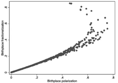
Figure 1presents the scatterplot of fractionalization versus
polarization using our data source. For low levels of fraction-alization, the correlation with polarization is positive, while for intermediate levels of fractionalization, the correlation is zero. For high levels of fractionalization, the correlation with polarization becomes negative. Therefore, the correlation is low when there is a high degree of heterogeneity. Generally speaking, if the number of groups is larger than two, the
existence of many small groups increases fractionalization but reduced polarization.
4. DATA
This study covers the period during 1960–2010. Data on migrant stocks—the number of people born in a country other than that in which they live—are taken from the World Bank for the 1960–2000 period,5and recently integrated throughout 2013.6The 1960–2000 dataset uses as a primary source of the raw data the United Nations Population Division’s Global Migration Database, created through the collaboration of the United Nations Population Division, the United Nations Statistics Division, the World Bank, and the University of Sus-sex. The estimates are derived from over 1,100 national indi-vidual census and population register records for more than 230 destination countries and territories over five decades. Each census round was conducted during a 10-year window, as most destination countries conducted their censuses at the turn of the decade.7 Ratha, Eigen-Zucchi, and Plaza (2016)
extend the UN Population Division (UNPD) dataset through-out 2013 using data from new censuses and country sources from Sub-Saharan Africa, Latin America and the Caribbean. We refer the interested reader toRatha and Shaw (2007)and
Rathaet al. (2016)for a thorough description of the method-ology and a more comprehensive overview than we can possi-bly give here. These studies also discuss the comparability of migrants’ statistics and the caveats on the underlying bilateral migration data, including the lack of standardized definitions and common reporting standards.8 O¨ zdenet al. (2011) offer an in-depth analysis of the data and show that migration from the South (developing countries) to the North (developed countries) increased from 14 million to 60 million during 1960–2000, mostly driven by movements to the US, Western Europe, and the Persian Gulf. However, South-South migra-tion remains the major share of total world migramigra-tion, although it is declining: in 1960, South-South migration accounted for about 61% of the total migrant stock, while it decreased to 48% by the year 2000.
We have a maximum of 135 countries, of which 27 are high-income economies according to the definition of the World Bank as of July 1, 2015 (seeTable A1 in the Online Appendix
for more information). Information on per capita GDP (PPP converted at 2005 constant prices) comes from the Penn World Table (PWT), version 7.1.7. From the same dataset we also take the population; the investment share of GDP, which is a proxy for capital; the government consumption share of GDP and the trade to GDP ratio, as the empirical growth lit-erature suggests that government intervention and a country’s openness to global economy and global trade have an impact on output growth (see, for example,Durlauf & Quah, 1999). To incorporate an indicator of human capital, we add the average years of school attainment of the population aged 25 and over fromBarro and Lee (2013). This is a fairly stan-dard set of economic growth predictors (see e.g.,Barro, 1991; Barro & Sala-i-Martin, 1992). We also include two dummy variables taking on the value of one for Latin American and Sub-Saharan countries, respectively. Finally, a recent work byAlesina, Michalopoulos, and Papaioannou (2016)uncovers a strong negative relation between ethnic inequality, measured as the within-country differences in well-being across ethnic groups, and per capita GDP. This very novel index of ethnic inequality is constructed by combining ethnographic and lin-guistic maps on the location of groups with satellite images of light density at night. Interestingly, when they include both
[image:5.595.40.282.561.730.2]the ethnic inequality index and the standard fragmentation indicators in the empirical specification, the latter loses signif-icance. We therefore explore whether our indices of birthplace fractionalization and polarization have independent and sig-nificant effects on economic performances, after controlling for inequality across ethnic lines.9
[image:6.595.42.563.598.736.2]We consider a global sample as well as two sub-samples, made up of developing and developed economies, using the classification of the World Bank as of July 1, 2015. We express the growth rates of per capita GDP and the diversity indices in percentage points so as to facilitate the interpretation of the coefficients of diversity in the empirical analysis. We transform all the other continuous variables into logs, except the growth rate of population and the index of ethnic inequality, to scale down the variance and reduce the effect of outliers.
Table 1contains the summary statistics of the full sample. Fractionalization has an average value of 0.11 and a larger standard deviation, 0.13. Polarization displays a mean and a standard deviation of virtually the same size, 0.17 and 0.18 respectively, but larger than those of fractionalization. Finally, while both indices have a minimum real value close to 0, when a country is extremely homogeneous (e.g., Vietnam, China), fractionalization has a maximum value of about 0.85 (e.g., Kuwait, Saudi Arabia) while polarization’s maximum value is 0.76 (e.g., Israel, Saudi Arabia) as also shown inFigure 1. InTable 2we report the between and within standard devia-tions. As we can see, the size of the within variation, although less than half the size of the between variation, as one would expect, is nonetheless critical and reflects within-country vari-ations in ethnic, social, and religious composition over time.
5. EMPIRICAL STRATEGY
Our baseline empirical model builds on a large literature that uses country-level data and cross-country regressions to explore the drivers of economic growth. We extend growth models as in Barro (1991) and Mankiw, Romer, and Weil (1992)by including a measure of diversity and estimate models of the following form:
gi¼aþcyi;t0þkDiviþx0ibþi ð3Þ
where giis the annual percentage growth rate of the (PPP
Con-verted) per capita GDP at 2005 constant prices in country i over a specific time interval (e.g., during 1960–2010)10; Divi
is i’s annual percentage growth rate in its level of diversity, measured by either fractionalization or polarization, over the same period11; xi is a vector of exogenous explanatory
variables that includes the level of income, investment share, population growth rate, average years of schooling, govern-ment consumption, trade openness, all measured in the initial year of each sub-period; xialso includes the ethnic inequality
index of Alesina et al. (2016)and dummies for countries in Latin America and Sub-Saharan Africa; ais a constant and
iis an error term. Our main coefficient of interest isk, which
describes the relationship between changes in diversity and economic development.
Our data on migration stocks are organized in 10-year inter-vals from 1960 to 2010; therefore, to fully exploit this dataset, we consider four different time windows and estimate model
(3) over the intervals 1960–2010, 1970–2010, 1980–2010, 1990–2000, and 2000–10. This allows us to take into account the changing nature of societies over time and to remove at the same time short-term fluctuations in the growth rate. We control for heteroskedasticity by reporting robust standard errors.
An important issue with model(3)is the likely endogeneity of diversity and thereby the Ordinary Least Squares (OLS) estimation ofEqn. (3)can be biased and inconsistent. Endo-geneity can arise as results of causality running both ways, e.g., countries that have higher growth rate might attract more immigrants from a variety of origins, thereby increasing the degree of diversity. Therefore, the heterogeneity of the popu-lation can be the effect rather than the cause of economic growth. Likewise, diversity can be endogenous because it is correlated with an omitted variable.12 In this paper, we address both issues by using two different strategies. The first strategy builds on a recent work by Docquier, Lodigiani, Rapoport, and Schiff (2015) and exploits the dyadic nature of our dataset on migration to run a gravity model and predict countries’ bilateral migration stocks out of a set of exogenous dyadic variables. We then use the bilateral predicted immigra-tion stocks to construct indices of fracimmigra-tionalizaimmigra-tion and polar-ization; finally, we use these gravity-based predicted diversity indices as instruments for birthplace diversity (fractionaliza-tion and polariza(fractionaliza-tion).
We pool data from 1960 to 2010 and estimate the following gravity model of bilateral migration stocks:
logðmÞij¼fiftþfjftþftþx0ijbþeij ð4Þ
where logðmÞijis the logarithm of the total number of foreign people living in country j and born in country i, fi ft is the
interaction between the country of origin fixed effect and year dummies; fjftis the interaction between the country of
desti-nation fixed effect and year dummies; ftis the time fixed effect;
xijis a vector of exogenous dyadic variables that includes some
Table 1. Summary statistics
Variable Mean Std. Dev. Min Max Obs
Fractionalization 0.11 0.13 0.00 0.85 1061
Polarization 0.17 0.18 0.00 0.76 1061
Per capita GDP 8.29 1.28 5.19 11.38 922
Schooling 1.70 0.62 0.01 2.67 828
Investments (% GDP) 2.99 0.60 0.36 4.54 922
Openness (% GDP) 4.02 0.74 0.65 6.01 922
Gov’t consumption (% GDP) 2.27 0.66 1.13 4.19 922
Population growth rate 1.83 1.25 1.28 9.85 884
Ethnic inequality 0.43 0.26 0.00 0.97 1007
Latin American countries 0.18 0.38 0.00 1.00 1061
Sub-Saharan countries 0.26 0.44 0.00 1.00 1061
classical impediments or facilitating factors in a list of gravity controls, in particular: a dummy for contiguous states; binary variables taking value one if i and j are in a colonial relation-ship, had the same colonizer, have a common language, or were parts of the same country in the past;eijis the error term.
We also include the log of the country of origin’s population and the capital-to-capital distance.13 To increase the predic-tive power of the gravity model, we follow Docquier et al. (2015) and include interactions between geographic distance and time dummies. These additional controls introduce time variation in model (4)so that identification comes also from time-varying factors. Moreover, these interactions are meant to capture changes in transportation and communication costs, which are likely to affect decisions to move from one country to another. The estimated gravity model allows us to construct predicted diversity indices, which are used as instruments for fractionalization and polarization in the cross-country regressions. Predictions of bilateral migration are calculated by means of a log-linear model and OLS estima-tor as inFrankel and Romer (1999). To deal with the presence of zero observations (when same pairs of countries do not have bilateral migration flows) we transform the dependent variable by adding 1. To avoid the bias of a log-transformation and check the robustness of our results, we also use the pseudo-poisson maximum likelihood estimator (PPML) suggested bySantos Silva and Tenreyro (2006).14
In a prominent paper,Rodriguez and Rodrik (2001)argue that this predicted instrument could act as a proxy for geogra-phy’s direct effect on growth and that omitting other channels through which geography affects growth may invalidate the exclusion restrictions. To exclude the possibility that our results are not spurious and are not arising from correlations of our indices with omitted factors, we extend the vector of controls in the two-stage least squares (2SLS) models by including the following variables: area in km2, altitude, mean distance to coast, mean distance to river, percentage of land area in the Tropics, an indicator for irrigation condition and a measure for soil quality. Results from these additional mod-els are reported inTables A2–A3 in the Online Appendix.15
Another potential concern is the inclusion of country of des-tination fixed effects in model (4). Ortega and Peri (2014)
argues that, by absorbing all the country-specific factors that account for bilateral flows, the presence of fixed effects may re-introduce endogeneity when e.g., they are correlated with the expected income levels in the target country. One solution would be the exclusion of country of destination fixed effects from the gravity model. However, although the resulting pre-dictors could be more credibly exogenous, the goodness of fit of the model is greatly deteriorated, and so is its ability to pre-dict the migration stocks in the data.16A much poorer model fit inevitably leads to weak instruments. In fact, as one would expect, we find that in all model specifications the predicted diversity indices are only weakly correlated to the endogenous variables. Moreover, critical values for first-stage F-stat are never above conventional levels characterizing weak instru-ments. Eventually, we chose the model that controls for coun-try dummies, as it explains more accurately global bilateral migration data and thus provides more robust instruments.
To further address the issue of omitted variable bias, our second strategy consists in estimating a dynamic panel data model a` la Arellano and Bover (1995) and Blundell and Bond (1998). This model removes country-specific unobserved factors that might drive the relationship between diversity and economic growth and takes additionally into account the potential endogeneity of the other explanatory variables. We use both internal instruments (that is, all available lags) as well as changes in the predicted values of fractionalization and polarization as instruments for the actual changes in these indices.17 We estimate this model using our 10-year interval data and all our explanatory variables—with the exception of fractionalization and polarization—are lagged one period (10 years). We do not include the ethnic inequality index in this specification, as it is time invariant. We use the two-step procedure proposed byArellano and Bond (1991)and obtain robust standard errors using the Windmeijer’s (2005) finite sample correction.
6. RESULTS
Our first round of results, obtained when we estimate a naı¨ve OLS model, is reported inTable 3. We consider different time intervals in each column and splitTable 3into two parts, Panel A which shows the impact of Fractionalization and Panel B the impact of Polarization.18
Before discussing our main explanatory variables, we briefly comment on the results with regard to the control variables. Overall, the control variables add significantly to the fit of the model and their signs are aligned with the mainstream studies on the determinants of growth (see e.g.,Barro, 1991; Mankiwet al., 1992). For example, whereas the average years of schooling and the rate of investment have a positive associ-ation with growth, initial income is negative as expected. This is the result of the so-called ‘‘conditional convergence”, i.e., poorer economies’ per capita incomes growth at a faster rate than richer economies. Some of the control variables fail to achieve significance at conventional levels when we look at the shortest time intervals (e.g., 2000–10), thus suggesting that initial endowment of production factors mostly affects the medium and long-run rate of economic growth. Finally note that ethnic inequality, the economic differences between ethnic groups coexisting in the same country, is indeed negative and significant asAlesinaet al. (2016)point out.
Table 3contains our baseline growth regressions for the per-iod 1960–2010. As it is made clear, diversity measured by either fractionalization or polarization is consistently positive and significant at conventional level. We obtain parameter estimates of similar magnitude and same significance for the periods 1970–2010, 1980–2010, and 1990–2010. The only nota-ble exception is the last decade, 2000–10, where fractionaliza-tion and polarizafractionaliza-tion are both negative, but only the latter is statistically different from zero, albeit only weakly.
[image:7.595.33.283.88.136.2]The coefficients allow for a direct reading and imply that, for example, during 1960–2010, the growth rate of the per cap-ita GDP increases by about 0.15 percentage points when the growth rate of fractionalization variable increases by one unit (i.e., one percentage point, approximately the increase experi-enced by Haiti). Similarly, one percentage point increase in the growth rate of polarization (similar to the change occurred in Djibouti during the period 1960–2010) is correlated with an increase of the per capita GDP of about 0.15 percentage points. Yet, one may be concerned with the potential unmea-sured heterogeneity between countries and the likely presence of reverse causality. The economic conditions in the potential
Table 2. Between and within standard deviation for fractionalization and polarization index
Variable Overall Between Within
Fractionalization 0.13 0.12 0.05
Polarization 0.18 0.16 0.07
country of destination, as well as its immigration policies, could be important drivers of immigration and if unaccounted for, they could bias our results and lead to incorrect infer-ences. InTable 4we therefore examine whether the estimated effects of diversity are robust to an instrumental variable approach, where the instrument builds on a gravity model of migration, as described in Eqn.(4).
Despite the fundamentally different procedure, the sign of the coefficients is unchanged and remains largely supportive of our previous results. Both fractionalization and polariza-tion now retain a positive sign and the substantive effect of diversity overall is now bigger: on average a one-point increase in the degree of fractionalization (polarization) is predicted to increase the per capita GDP by about 0.25 (0.26) percentage points on average. The other contextual covariates behave lar-gely as inTable 3. Note however that diversity is significant at conventional levels only over long time intervals. In fact, dur-ing 1990–2010 as well as durdur-ing 2000–10, both indices,
although consistently positive, are insignificant. This result may also stem from the nature of the specific subsamples under examination, i.e., diversity may have not been affecting economic growth when we restrict the sample to the two most recent decades. Note also that the results in the last two col-umns are subject to an important caveat: the values of the
F-stat are all below conventional levels characterizing weak instruments. As such, these results must be interpreted with caution.
Tables 5 and 6 present analogous estimates ofTable 4but distinguish between developing (Table 5) and developed (Table 6) countries. Results for developing countries inTable 5
[image:8.595.47.560.79.494.2]are largely consistent with those inTable 4, and both fraction-alization and polarization seem to matter for economic growth over long time intervals. The size of both indices is now larger, and a shift of one percentage point in the level of diversity produces, on average, an increase in per capita income of about 0.3 percentage points. However, when we turn to the
Table 3. Growth and diversity—OLS results
60–10 70–10 80–10 90–10 00–10
Panel A
Fractionalization 0.148*** 0.113*** 0.131*** 0.061* 0.040
(0.046) (0.042) (0.039) (0.033) (0.024)
Per capita GDP, t0 1.127*** 0.957*** 0.968*** 0.677*** 1.208***
(0.171) (0.139) (0.156) (0.203) (0.197)
Population growth rate 0.374** 0.195 0.275* 0.287* 0.515**
(0.181) (0.150) (0.152) (0.159) (0.221)
Investments (% GDP) 0.551*** 0.385* 0.132 0.511 0.598
(0.152) (0.230) (0.277) (0.309) (0.436)
Schooling 0.882*** 0.938*** 1.038*** 0.495 0.824
(0.291) (0.285) (0.374) (0.521) (0.638)
Openness (% GDP) 0.182 0.147 0.029 0.044 0.231
(0.154) (0.157) (0.203) (0.244) (0.427)
Gov’t consumption (% GDP) 0.122 0.082 0.116 0.289 0.067
(0.125) (0.192) (0.222) (0.322) (0.428)
Ethnic inequality 0.969* 0.863 1.057* 0.000*** 1.024
(0.546) (0.587) (0.624) (0.000) (0.821)
Observations 95 118 118 127 135
R2 0.607 0.505 0.456 0.307 0.369
Panel B
Polarization 0.152*** 0.113** 0.132*** 0.062* 0.042*
(0.047) (0.043) (0.040) (0.033) (0.025)
Per capita GDP, t0 1.114*** 0.939*** 0.946*** 0.664*** 1.220***
(0.171) (0.138) (0.156) (0.203) (0.196)
Population growth rate 0.389** 0.190 0.266* 0.278* 0.523**
(0.176) (0.149) (0.150) (0.159) (0.218)
Investments (% GDP) 0.548*** 0.382 0.124 0.510 0.599
(0.153) (0.230) (0.276) (0.309) (0.435)
Schooling 0.867*** 0.933*** 1.036*** 0.494 0.831
(0.291) (0.286) (0.374) (0.521) (0.637)
Openness (% GDP) 0.191 0.153 0.039 0.041 0.238
(0.155) (0.158) (0.204) (0.244) (0.426)
Gov’t consumption (% GDP) 0.120 0.074 0.106 0.285 0.071
(0.124) (0.192) (0.221) (0.321) (0.427)
Ethnic inequality 0.944* 0.862 1.053* 0.000*** 1.024
(0.547) (0.588) (0.624) (0.000) (0.819)
Observations 95 118 118 127 135
R2 0.606 0.503 0.455 0.306 0.370
developed economies, inTable 6, both indices are indiscernible from zero, with the exception of the last decade, 2000–10, where they are negative and significant. Overall, it appears that developing countries are those benefiting from diversity, perhaps because they are more distant from the technological frontier (see e.g.,Vandenbusscheet al., 2006). Yet, the results inTables 5 and 6 must also be viewed with caution because most of the models are run on small samples and have low first-stageF-stat, in particular the models estimated over short time periods.19
To delve deeper into the heterogeneous effects of diversity on growth, Table 7 reports dynamic panel data estimators, which should further address endogeneity concerns and at them same time it is based on larger samples.20 The results suggest that diversity increases the level of per capita income in the full sample, as well as in the sample of developing countries. In fact, in the sample of more advanced
econo-mies, we cannot reject the null of no impact of diversity in the GDP. If anything, this corroborates our previous findings on the different effect of diversity on growth, according to the level of development. The coefficients are considerably smal-ler, about one third of those in Tables 5 and 6, but this is unsurprising as this last model, by introducing a battery of instruments to reduce the omitted variable bias, is expected to produce very conservative estimates. As we can see, an increase of one percentage point in the degree of fractional-ization (polarfractional-ization) increases the per capita output by a minimum of 0.087 (0.095) percentage points in the full sam-ple to a maximum of 0.095 (0.096) percentage points in the sample of developing economies. Once again, the signs of the coefficients consistently point out to a similar effect of fractionalization and polarization on economic growth. This result stands in sharp contrast to previous studies by e.g.,
[image:9.595.39.549.79.519.2]Alesina et al. (2003) and Ager and Bru¨ckner (2013), which
Table 4. Growth and diversity—2SLS results
60–10 70–10 80–10 90–10 00–10
Panel A
Fractionalization 0.209** 0.270*** 0.273*** 0.123 0.025
(0.082) (0.089) (0.095) (0.168) (0.153)
Per capita GDP, t0 1.206*** 1.100*** 1.028*** 0.686*** 1.268***
(0.170) (0.158) (0.161) (0.195) (0.218)
Population growth rate 0.382** 0.141 0.242 0.281* 0.596**
(0.194) (0.185) (0.173) (0.165) (0.240)
Investments (% GDP) 0.547*** 0.363* 0.100 0.445 0.481
(0.145) (0.217) (0.266) (0.307) (0.479)
Schooling 0.915*** 0.977*** 0.991** 0.420 0.625
(0.280) (0.314) (0.397) (0.561) (0.795)
Openness (% GDP) 0.222 0.131 0.018 0.040 0.168
(0.140) (0.143) (0.203) (0.230) (0.389)
Gov’t consumption (% GDP) 0.132 0.046 0.122 0.316 0.070
(0.115) (0.191) (0.222) (0.318) (0.402)
Ethnic inequality 0.887 0.850 1.123* 0.000*** 0.798
(0.546) (0.611) (0.643) (0.000) (0.878)
Observations 95 118 118 127 135
R2 0.595 0.422 0.372 0.283 0.335
First stage F-stat 45 49 13 4 3
Panel B
Polarization 0.221** 0.281*** 0.281*** 0.126 0.027
(0.086) (0.092) (0.097) (0.170) (0.156)
Per capita GDP, t0 1.195*** 1.066*** 0.983*** 0.659*** 1.261***
(0.168) (0.156) (0.161) (0.195) (0.197)
Population growth rate 0.404** 0.127 0.221 0.263 0.592***
(0.188) (0.185) (0.172) (0.174) (0.227)
Investments (% GDP) 0.543*** 0.353 0.081 0.443 0.480
(0.147) (0.219) (0.266) (0.308) (0.478)
Schooling 0.897*** 0.966*** 0.986** 0.415 0.619
(0.280) (0.317) (0.398) (0.560) (0.804)
Openness (% GDP) 0.238* 0.145 0.038 0.034 0.163
(0.141) (0.144) (0.207) (0.230) (0.389)
Gov’t consumption (% GDP) 0.129 0.023 0.101 0.309 0.067
(0.114) (0.193) (0.220) (0.314) (0.405)
Ethnic inequality 0.844 0.847 1.117* 0.000*** 0.796
(0.553) (0.616) (0.647) (0.000) (0.874)
Observations 95 118 118 127 135
R2 0.592 0.412 0.366 0.282 0.333
First stage F-stat 44 49 25 4 3
found that fractionalization and polarization have an oppo-site impact on output growth.
7. CONCLUSIONS
In this article we explore whether diversity brought about by immigration affects economic development. This issue lies at the intersection of two separate yet intertwined strands of research: one on diversity and the other on migration. The issue of migration is rising quickly up the global agenda
[image:10.595.48.559.79.302.2]and features prominently in the academic literature, where a remarkable consensus has emerged around the beneficial impact of immigration on the economic development of the host country. At the same time the literature on diver-sity has so far found difficult to convincingly establish the very direction of the effect of cultural heterogeneity on eco-nomic growth (that is whether it is positive or negative). It is also unclear to what extent fractionalization and polariza-tion differ in their effects on output growth and which index is more relevant as a determinant of economic outcomes. Perhaps more importantly, however, existing contributions
Table 5. Growth and diversity—2SLS results, developing countries
60–10 70–10 80–10 90–10 00–10 60–10 70–10 80–10 90–10 00–10
Fractionalization 0.277*** 0.340*** 0.335*** 0.248 0.092 (0.093) (0.101) (0.108) (0.188) (0.242)
Polarization 0.288*** 0.352*** 0.345*** 0.255 0.097
(0.097) (0.104) (0.111) (0.195) (0.258) Per capita GDP, t0 1.181*** 1.150*** 1.026*** 0.736*** 1.230** 1.179*** 1.141*** 1.005*** 0.718*** 1.225**
(0.228) (0.263) (0.255) (0.264) (0.541) (0.232) (0.268) (0.258) (0.264) (0.538) Population growth 0.639** 0.245 0.296 0.439* 1.083* 0.642** 0.239 0.286 0.421* 1.081* (0.267) (0.279) (0.251) (0.246) (0.564) (0.265) (0.276) (0.251) (0.245) (0.567) Investments (% GDP) 0.445*** 0.369 0.038 0.406 0.429 0.452*** 0.375 0.043 0.412 0.435
(0.148) (0.275) (0.350) (0.328) (0.569) (0.150) (0.276) (0.352) (0.329) (0.565) Schooling 0.894** 0.932** 0.887* 0.014 0.332 0.886** 0.927** 0.880* 0.023 0.328
(0.353) (0.403) (0.500) (0.769) (1.213) (0.357) (0.405) (0.504) (0.766) (1.233) Openness (% GDP) 0.260 0.043 0.100 0.298 0.761 0.266 0.048 0.091 0.291 0.750 (0.168) (0.164) (0.240) (0.287) (0.564) (0.168) (0.165) (0.243) (0.289) (0.577) Gov’t consumption 0.133 0.088 0.012 0.327 0.015 0.133 0.092 0.013 0.328 0.013
(0.129) (0.228) (0.257) (0.336) (0.451) (0.129) (0.230) (0.259) (0.336) (0.454) Ethnic inequality 0.235 0.638 0.915 0.359 1.521 0.215 0.634 0.913 0.364 1.504
(0.691) (0.844) (0.849) (0.813) (0.947) (0.695) (0.852) (0.856) (0.818) (0.974)
Observations 73 93 93 100 108 73 93 93 100 108
First stage F-stat 35 19 9 4 1 34 19 17 4 1
*p< 0.10,**p< 0.05,***p< 0.01. Huber–White robust standard errors in parentheses. Dummies for Latin American and Sub-Saharan countries and a constant are included but not shown.
Table 6. Growth and diversity—2SLS results, developed countries
60–10 70–10 80–10 90–10 00–10 60–10 70–10 80–10 90–10 00–10
Fractionalization 0.034 0.042 0.086 0.137 0.428** (0.090) (0.089) (0.151) (0.181) (0.190)
Polarization 0.035 0.042 0.087 0.133 0.400***
(0.092) (0.088) (0.152) (0.176) (0.146) Per capita GDP, t0 1.613*** 1.787*** 1.663** 1.893*** 0.717 1.595*** 1.779*** 1.617** 1.883*** 0.331 (0.286) (0.592) (0.691) (0.618) (0.963) (0.299) (0.607) (0.674) (0.651) (0.833) Population growth 0.086 0.247 0.436 0.547** 0.303 0.080 0.247 0.439 0.581** 0.344* (0.173) (0.180) (0.276) (0.260) (0.248) (0.174) (0.184) (0.271) (0.280) (0.204) Investments (% GDP) 0.224 0.397 0.758* 1.393** 2.766** 0.218 0.391 0.802** 1.569** 2.654** (0.369) (0.334) (0.387) (0.660) (1.335) (0.369) (0.339) (0.396) (0.706) (1.167) Schooling 0.281 0.090 0.227 0.006 4.097* 0.293 0.088 0.265 0.215 1.904 (0.474) (0.350) (0.844) (1.260) (2.350) (0.464) (0.350) (0.870) (1.031) (1.554) Openness (% GDP) 0.407*** 0.514*** 0.482 0.948*** 0.367 0.410*** 0.522*** 0.444 0.916*** 0.234
(0.118) (0.175) (0.345) (0.342) (0.369) (0.122) (0.177) (0.328) (0.349) (0.351) Gov’t consumption 0.241 0.712 0.986 0.672 0.658 0.228 0.682 1.095 0.879 0.056 (0.262) (0.469) (0.821) (0.691) (1.064) (0.251) (0.457) (0.747) (0.542) (0.686) Ethnic inequality 0.355 0.149 0.465 0.260 2.991*** 0.351 0.157 0.437 0.467 1.529
(0.565) (0.593) (0.665) (0.834) (1.107) (0.580) (0.596) (0.628) (0.718) (1.152)
Observations 22 25 25 26 27 22 25 25 26 27
First stage F-stat 5 10 6 2 3 6 10 6 3 5
*
[image:10.595.48.559.363.585.2]have assumed that diversity exerts the same effect on eco-nomic growth both over time and across countries and, to date, there has been no systematic attempt to explore whether diversity has idiosyncratic effects on economic growth.
Against this background, first, we use a new dataset on migrant stocks, based on population censuses, which gives us the opportunity to compute time-varying measures of frac-tionalization and polarization during 1960–2010. Second, we compare and contrast developing and developed economies to investigate whether there are systematic differences between them. We employ an array of econometric models over five sub-periods, including a novel instrumental variable approach, to account for the likely omission of important co-determinants of growth and diversity and mitigate concerns of reverse causality.
We find that our indices of cultural heterogeneity, birthplace fractionalization, and polarization, have a positive impact on the growth rate of the GDP over large time periods, and that they coefficients are of similar magnitude. By splitting coun-tries into two subgroups according to their initial level of per capita income, our results reveal that developing econo-mies seem to be more likely to experience an increase in the GDP growth rate following changes in the degree of diversity. Although this finding challenges the assumption of a homoge-nous effect of diversity on growth, on which the majority of the cross-country empirical literature on diversity is based, it is subject to some caveats, in particular the quality of the first stage regression in the models run over the shortest time peri-ods. Overall, the results of our most conservative model—i.e., panel data model—suggest that one percentage point increase in the growth rate of fractionalization (polarization) boosts the per capita output by about 0.1 percentage point in the developing countries.
[image:11.595.40.551.79.312.2]In the words ofAlesinaet al. (2003, p. 182): ‘‘The question of what makes different countries more or less successful eco-nomically and what explains the quality of their policies is one of the most fascinating that economists can ask, but it is also one of the most difficult to answer.”We hope that our research could make a contribution to successfully addressing this dif-ficult question. Whereas we provide new important insights into the effect of cultural heterogeneity on economic growth—and our evidence seems to suggest that immigration-fueled diversity is generally good for economic growth—more needs to be done to fully uncover the effect of diversity on development. Firstly, diversity is a phe-nomenon continually in motion and difficult to conceptualize. Individuals have many observable characteristics—race, lan-guage, religion, nationality, wealth, education-but only some categories have economic salience. Indices based on the ethnic-ity, religion, or language identity of sub-populations within each country could be too narrow, whereas these identities are usually given at birth, asHorowitz (1985)suggests. If we subscribe to Horowitz’s (1985) claim that the ascription to birth is one of the most coherent marker of diversity, future studies should treat migration and diversity as two phenomena belonging to the same line of inquiry. Secondly, although we extend earlier research on diversity by constructing more informative measures of birthplace heterogeneity, future research should focus on the characteristics of the migrants (e.g., age, education), which can give a more systematic and accurate snapshot of diversity patterns. Thirdly, the theory on diversity and team performance relies on micro-level argu-ments that focus on individual behavior. To dig deeper into the relationship between diversity and growth, more effort should be devoted to the integration of macro data with individual-level information on cultural and social characteris-tics.
Table 7. Growth and diversity—dynamic panel results
All countries Developing countries Developed countries
Fractionalization 0.087** 0.095** 0.104
(0.043) (0.042) (0.146)
Polarization 0.089** 0.096** 0.119
(0.043) (0.043) (0.150)
Per capita GDP 0.127 0.144 0.431 0.443 4.577** 4.597**
(0.514) (0.510) (0.640) (0.641) (2.186) (2.054)
Investments (% GDP) 2.011*** 2.018*** 1.931*** 1.921*** 0.178 0.340
(0.502) (0.506) (0.596) (0.600) (1.592) (1.130)
Schooling 0.987 1.008 1.777* 1.787* 0.455 0.131
(0.881) (0.878) (0.953) (0.957) (2.592) (2.663)
Population growth rate 0.253 0.248 0.447 0.456 0.465 0.591
(0.392) (0.391) (0.423) (0.425) (0.982) (0.857)
Openness (% GDP) 0.521 0.504 0.376 0.356 0.483 0.566
(0.698) (0.692) (0.754) (0.757) (1.001) (0.849)
Gov’t consumption (% GDP) 2.154*** 2.171*** 1.791* 1.793* 0.368 0.202
(0.783) (0.784) (0.959) (0.962) (1.627) (2.042)
Observations 466 466 367 367 99 99
Countries 130 130 103 103 27 27
AR(1)p-value 0.000 0.000 0.000 0.000 0.551 0.520
AR(2)p-value 0.859 0.872 0.568 0.557 0.603 0.581
Hansen testp-value 0.622 0.620 0.462 0.451 0.261 0.326
NOTES
1. Alesinaet al. (2003), for example, compute linguistic fractionalization
using data from the Encyclopedia Britannica, which reports the shares of languages spoken as mother tongues, usually based on national census. Data on ethnic fractionalization were also computed using as a primary source the Encyclopedia Britannica, integrated with data from other sources such as the CIA World Factbook. Subsequent studies build on the same data.
2. Some key points distinguish our empirical efforts from theirs: (i) we provide the first systematic analysis of the differences in the impact of diversity on growth between developing and developed countries; (ii) we address the issue of omitted variable bias using a battery of gravity-based instrumental variables and extend the analysis to the 2000–10 decade; and (iii) we compute indices of population diversity and distinguish between fractionalization and polarization, which has been found to be crucial ‘‘when examining the effects that cultural diversity has on economic growth” (Ager & Bru¨ckner, 2013, p. 96), in particular in light of the important debate on how to capture effectively the degree of diversity within a country (see e.g.,Montalvo & Reynal-Querol, 2005a; Platteau, 2009). The effect of them all taken together leads to substantially different implications.
3. In a very recent contribution, however, Gisselquist, Leiderer, and
Nin˜o-Zarazu´a (2016)challenge the ‘‘conventional wisdom”maintaining a
negative relationship between ethnic heterogeneity and public goods provision and find that the relation is actually positive, in particular with key welfare outcomes.
4. This first measure of diversity, i.e., birthplace diversity, builds directly on the one used byOttaviano and Peri (2006). As such,pialso includes the natives.
5.
http://data.worldbank.org/data-catalog/global-bilateral-migration-database.
6. Two matrixes are available for the post-2000 decade and we use the most recent one as it covers a wider number of countries. Seehttp:// www.worldbank.org/en/topic/migrationremittancesdiasporaissues/brief/
migration-remittances-data.
7. Alesinaet al. (2016)use also information on whether migrants have a
college education. A richer dataset does exist but only captures the structure of migration to OECD destinations. See alsoArtuc¸, Docquier,
O¨ zden, and Parsons (2015) and Docquier and Rapoport (2012) for a
discussion on more refined brain drain indicators, including the estimates of gross and net human capital levels across the world.
8. To exclude the possibility that the relationship between diversity and economic growth is driven by the inclusion of the 2010 wave, we estimate models without 2010. The results are shown inTables A7–A10 in the
Online Appendix. Coefficients are slightly smaller but qualitatively
consistent with the baseline results.
9. We thank an anonymous referee for suggesting the inclusion of this variable.
10. The average of the annual growth rates is often used. This is a reasonable approximation to the compound growth rate, the one we use in this paper, for low rates but loses accuracy as the growth rate rises. However, in our data set the two measures show a very high correlation of 0.9.
11. We apply a 1% winsorization to the annual percentage growth rate of fractionalization and polarization so as to reduce the effect of extreme values.
12. Islam (1995), for example, shows that the production function
actually differs across countries and is correlated with the included explanatory variables, thus creating omitted variable bias.
13. Due to space limitations, the results of the gravity model of bilateral stocks are not presented here, but are available upon request from the authors.
14. Results from the two-stage least squares models when we use predicted diversity indices calculated from PPML as instruments are shown inTables A4–A6 in the Online Appendix.
15. Note that given the small number of degrees of freedom, we cannot provide the same estimates for the sample of developed economies.
16. In fact, we find that the adjustedR-squared of the gravity model without country of destination dummies is 0.33 while the value for the model which includes country dummies is 0.66. Likewise, we detect a 33% increase in the Root MSE between the two models.
17. For studies using panel data model, see Islam (1995). For recent applications of dynamic panel data model see Arcand, Berkes, and
Panizza (2015)andBeck and Levine (2004).
18. The correlation between fractionalization and polarization is 0.9, which suggests near multicollinearity. In fact, when we include both indices jointly in the regression, the estimators have very large variance and the confidence intervals are much wider, making precise estimation difficult. For this reason, we use each index separately.
19. Note also that the values of the F statistics in the last decade across the developed countries make the negative sign of diversity unreliable.
20. At the bottom ofTable 6we report the standard specification tests and show that most regressions reject the null of no first order autocorrelation, and that all models do not reject the null of no second order autocorrelation. The Hansen tests of the over-identifying restrictions never reject the null.
REFERENCES
Ager, P., & Bru¨ckner, M. (2013). Cultural diversity and economic growth:
Evidence from the US during the age of mass migration. European
Economic Review, 64, 76–97.
Alesina, A., Devleeschauwer, A., Easterly, W., Kurlat, S., & Wacziarg, R.
(2003). Fractionalization.Journal of Economic Growth, 8(2), 155–194.
Alesina, A., Harnoss, J., & Rapoport, H. (2016). Birthplace diversity and
economic prosperity.Journal of Economic Growth, 21(2), 101–138.
Alesina, A., & La Ferrara, E. (2005). Ethnic diversity and economic
performance.Journal of Economic Literature, 762–800.
Alesina, A. F., Michalopoulos, S., & Papaioannou, E. (2016). Ethnic
inequality.Journal of Political Economy(in press).
Arcand, J. L., Berkes, E., & Panizza, U. (2015). Too much finance?.