University of Warwick institutional repository:
http://go.warwick.ac.uk/wrap
A Thesis Submitted for the Degree of PhD at the University of Warwick
http://go.warwick.ac.uk/wrap/62527
This thesis is made available online and is protected by original copyright.
Please scroll down to view the document itself.
M A
E
G
NS I
T A T MOLEM
U N
IV
ER
SITAS WARWICEN
SIS
Functional Data Analysis in Phonetics
by
Pantelis-Zenon Hadjipantelis
Thesis
Submitted to the University of Warwick for the degree of
Doctor of Philosophy
Department of Statistics
Contents
List of Tables iv
List of Figures v
Acknowledgments vii
Declarations viii
Abstract ix
Abbreviations x
Chapter 1 Introduction 1
Chapter 2 Linguistics, Acoustics & Phonetics 9
2.1 Basic Computational Aspects ofF0 determination . . . 11
2.2 Tonal Languages . . . 16
2.3 Pitch & Prosody Models . . . 18
2.4 Linguistic Phylogenies . . . 21
2.5 Datasets . . . 23
2.5.1 Sinica Mandarin Chinese Continuous Speech Prosody Corpora (COSPRO) . . . 23
2.5.2 Oxford Romance Language Dataset . . . 25
Chapter 3 Statistical Techniques for Functional Data Analysis 28 3.1 Smoothing & Interpolation . . . 31
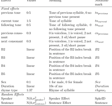
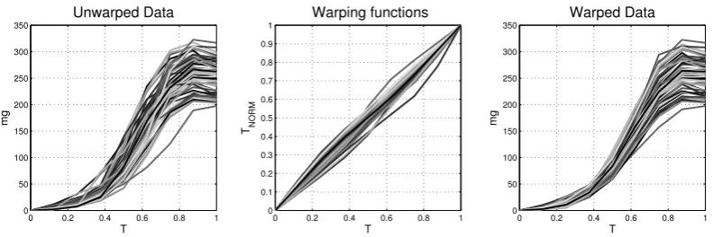
3.2 Registration . . . 34
3.2.1 A non-linguistic dataset . . . 38
3.2.2 Pairwise synchronization . . . 38
3.2.3 Area under the curve synchronization . . . 42
3.2.4 Self-modelling warping functions . . . 44
3.2.5 Square-root velocity functions . . . 47
3.3.1 Functional Principal Component Analysis . . . 51
3.4 Modelling Functional Principal Component scores . . . 53
3.4.1 Mixed Effects Models . . . 53
3.4.2 Model Estimation . . . 57
3.4.3 Model Selection . . . 59
3.5 Stochastic Processes and Phylogenetics . . . 64
3.5.1 Gaussian Processes & Phylogenetic Regression . . . 67
3.5.2 Tree Reconstruction . . . 70
Chapter 4 Amplitude modelling in Mandarin Chinese 73 4.1 Introduction . . . 73
4.2 Sample Pre-processing . . . 76
4.3 Data Analysis and Results . . . 77
4.4 Discussion . . . 90
Chapter 5 Joint Amplitude and Phase modelling in Mandarin Chi-nese 93 5.1 Introduction . . . 93
5.2 Phonetic Analysis of Mandarin Chinese utilizing Amplitude and Phase 94 5.3 Statistical methodology . . . 96
5.3.1 A Joint Model . . . 96
5.3.2 Amplitude modelling . . . 98
5.3.3 Phase modelling . . . 99
5.3.4 Sample Time-registration . . . 100
5.3.5 Compositional representation of warping functions . . . 101
5.3.6 Further details on mixed effects modelling . . . 102
5.3.7 Estimation . . . 104
5.3.8 Multivariate Mixed Effects Models & Computational Consid-erations . . . 105
5.4 Data Analysis and Results . . . 109
5.4.1 Model Presentation & Fitting . . . 109
5.5 Discussion . . . 116
Chapter 6 Phylogenetic analysis of Romance languages 119 6.1 Introduction . . . 119
6.2 Methods & Implementations . . . 122
6.2.1 Sample preprocessing & dimension reduction . . . 122
6.2.2 Tree Estimation . . . 130
6.2.3 Phylogenetic Gaussian process regression . . . 132
6.4 Discussion . . . 142
Chapter 7 Final Remarks & Future Work 146 Appendix A 172 A.1 Voicing of Consonants and IPA representations for Chapt. 4 & 5 . . 172
A.2 Comparison of Legendre Polynomials and FPC’s for Amplitude Only model . . . 173
A.3 Speaker Averaged Sample for Amplitude Only model . . . 174
A.4 Functional Principal Components Robustness check for Amplitude Only model . . . 175
A.5 Model IDs for Amplitude Only model . . . 176
A.6 AIC scores (ML-estimated models) for Amplitude Only model . . . . 177
A.7 Jackknifing for Amplitude Only model . . . 178
A.8 Estimate Tables for Amplitude Only model . . . 178
A.9 Covariates for Figures 4.5 and 4.6 . . . 190
A.10 Covariance Structures for Amplitude & Phase model . . . 191
A.11 Linguistic Covariate Information for Fig. 5.4 . . . 192
A.12 Numerical values of random effects correlation matrices for Amplitude & Phase model . . . 192
A.13 Warping Functions in Original Domain . . . 193
A.14 Area Under the Curve - FPCA / MVLME analysis . . . 193
A.15 FPC scores for digit one . . . 195
List of Tables
2.1 ToBi Break Annotation . . . 20
2.2 Covariates examined in relation toF0 production in Mandarin . . . 25
2.3 Speaker-related information in the Romance languages sample . . . 26
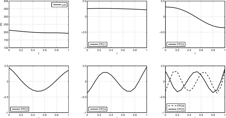
4.1 Individual and cumulative variation percentage per FPC. . . 80
4.2 Random effects standard deviation and parametric bootstrap confi-dence intervals . . . 83
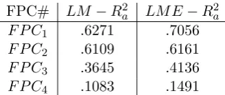
4.3 AdjustedR2 scores . . . . 88
5.1 Percentage of variances reflected from each respective FPC . . . 111
5.2 Actual deviations in Hz from each respective FPC . . . 111
5.3 Random effects std. deviations. . . 115
6.1 Individual and cumulative variation percentage per FPC. . . 130
6.2 MLE estimates for the hyperparameters in Eq. 6.23 for digit one . . 139
6.3 Posterior estimates for the parameters of Gjt0 for digit one at the root nodeω0 . . . 140
A.1 Auditory variation per LP . . . 173
A.2 Auditory variation per FPC in the Speaker-centerd sample . . . 175
A.4 Sample-wide AIC results . . . 178
A.5 F P C1 Fixed effects tables . . . 179
A.6 F P C2 Fixed effects tables . . . 181
A.7 F P C3 Fixed effects tables . . . 185
A.8 F P C4 Fixed effects tables . . . 188
A.9 Specific covariate information for theF0 curves in Fig. 4.5. . . 190
A.10 Specific covariate information for theF0 track in Fig. 4.6. . . 190
A.11 Covariate information for the estimated F0 track in Fig. 5.4 . . . 192
List of Figures
2.1 Male French speaker saying the word “un” (œ) . . . 12
2.2 CepstralF0 determination . . . 13
2.3 CepstralF0 determination employing different windows . . . 17
2.4 Reference tone shapes for Tones 1-4 as presented in the work of Yuen Ren Chao . . . 19
2.5 Tone realization in 5 speakers from the COSPRO-1 dataset. . . 24
2.6 Unrooted Romance Language Phylogeny based on [106] . . . 27
3.1 Three different types of variation in functional data . . . 36
3.2 Pairwise warping function example . . . 40
3.3 Pairwise warping of beetle growth curves . . . 41
3.4 Area Under the Curve warping example . . . 43
3.5 Area Under the Curve warping of beetle growth curves . . . 44
3.6 Self-modelling warping of beetle growth curves . . . 46
3.7 Square-root velocity warping of beetle growth curves . . . 49
3.8 Illustration of why LMMs can be helpful . . . 55
3.9 Illustration of a simple nested design . . . 56
3.10 Illustration of a simple crossed design . . . 57
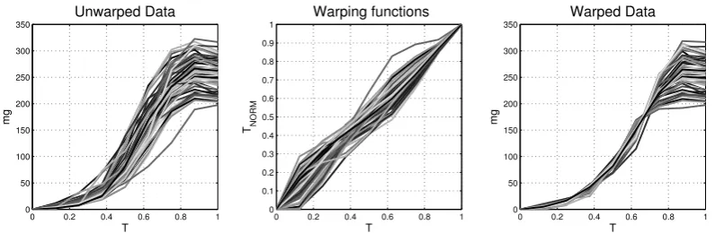
4.1 Schematic ofF0 reconstruction . . . 75
4.2 Covariance function of the 54707 smoothedF0 sample curves . . . . 78
4.3 FPCA results; Amplitude only model . . . 81
4.4 Tone Estimates . . . 88
4.5 One randomly selected syllable for each of the five tones . . . 89
4.6 Randomly chosenF0 trajectory over (normalized) time . . . 90
5.1 Triplet trajectories from speakersF02 &M02 over natural time . . 95
5.2 Random effects structure of the multivariate mixed effects model . . 104
5.3 Amplitude variation phase variation functions for Fig. 5.1 . . . 109
5.4 Model estimates over real time . . . 111
5.6 H (Phase) Functional Principal Components Ψ . . . 113
5.7 Random effects correlation matrices . . . 114
6.1 Unsmoothed and smoothed spectrogram of a male Portuguese speaker saying “un” ( ˜u(N) ) . . . 122
6.2 Unwarped and warped spectrogram of a male Portuguese speaker saying “un”(˜u(N)) . . . 127
6.3 Functional Principal Components for the digitone spectrograms . . 128
6.4 Median branch length consensus tree for the Romance language dataset133 6.5 Centred spectrogram for the Romance protolanguage . . . 141
A.1 Sample FPC’s normalized on L[0,1] . . . 173
A.2 Legendre polynomials in L[0,1] . . . 173
A.3 Covariance function for the Speaker-centred data . . . 174
A.4 Mean Function and 1st, 2nd, 3rd, 4th, 5th and 6th Functional Prin-cipal Components for the Speaker-centred data . . . 174
A.5 Expected value and inf/sup values for the 1st, 2nd, 3rd and 4th Functional Principal Components of COSPRO’s subsamples . . . 175
A.6 Bar-chart showing the relative frequencies of model selection under jackknifing . . . 179
A.7 Modes of variation in the original warping function space due to the components of the transformed domain . . . 193
A.8 WAU C (Amplitude) Functional Principal Components ΦAU C . . . 194
A.9 SAU C (Phase) Functional Principal Components ΨAU C . . . 194
A.10 Random effects correlation matrices under an AUC framework . . . 195
A.11 Mean spectrogram for the instances of digitone . . . 196
A.12 Empirical distribution of logged branch lengths retrieved from Tree-fam ver.8.0 . . . 196
A.13 Language specific spectrograms for the 5 languages used . . . 197
Acknowledgments
I was fortunate to come across people who helped me in this PhD, among those were: Alistair Tucker, Anas Rana, Ashish Kumar, Aude Exbrayat, Chris Knight, Chris Oates, Davide Pigoli, David Springate, Deborah Walker, Gui Pedro de Mendon¸ca, John Coleman, John Moriarty, John Paravantis, Jenny Bowskill, M´onica de Lucena, Nick Jones, Nikolai Peremezhney, Phil Richardson, Quentin Caudron, Robin Ball, Sergio Morales, Yan Zhou and a few anonymous referees.
Special thanks goes to Jonathan P. Evans and my family; while far away, each gave me guidance and courage to keep going.
Declarations
Parts of this thesis have been published or are in submission in:
• PZ Hadjipantelis, JAD Aston and JP Evans. Characterizing fundamental frequency in Mandarin: A functional principal component approach utilizing mixed effect models, Journal of the Acoustical Society of America, Volume 131, Issue 6, pp. 4651-4664 (2012)
• PZ Hadjipantelis, NS Jones, J Moriarty, D Springate and CG Knight. Function-Valued Traits in Evolution,Journal of the Royal Society Interface, Volume 10, No 82, 20121032, (2013)
• PZ Hadjipantelis, JAD Aston, H-G M¨uller and J Moriarty. Analysis of spike train data: A Multivariate Mixed Effects Model for Phase and Amplitude, (2013) (Accepted for publication in the Electronic Journal of Statistics)
• PZ Hadjipantelis, JAD Aston, H-G M¨uller and JP Evans. Unifying Am-plitude and Phase Analysis: A Compositional Data Approach to Functional Multivariate Mixed-Effects modelling of Mandarin Chinese, (2013) ( http: //arxiv.org/abs/1308.0868)
Abstract
Abbreviations
AIC Akaike Information Criterion AUC Area Under the Curve
BIC Bayesian Information Criterion CDF Cumulative Distribution Function
COSPRO Mandarin COntinuous Speech PROsody Corpora DCT Discrete Cosine Transform
DFT Discrete Fourier Transform DTW Dynamic Time-Warping DWT Discrete Wavelet Transform EEG Electroencephalography FDA Functional Data Analysis
FPCA Functional Principal Component Analysis FFT Fast Fourier Transform
F0 Fundamental Frequency
GMM Gaussian Mixture Model GPR Gaussian Process Regression HMM Hidden Markov Model
ICA Independent Component Analysis
INTSINT INternational Transcription System for INTonation IPA International Phonetic Alphabet
JND Just Noticeable Difference K-L Kullback-Leibler (divergence) LMM Linear Mixed-effects Model MAP Maximum A Posterior MCMC Markov Chain Monte Carlo MDL Minimum Description Length MLE Maximum Likelihood Estimate MOMEL MOd´elisation de MELodie
MVLME Multi-Variate Linear Mixed Effect (model) qTA quantitative Target Approximation
O-U Ornstein-Uhlenbeck (process)
PACE Principal Analysis by Conditional Estimation PDF Probability Density Function
PCA Principal Component Analysis
PGPR Phylogenetic Gaussian Process Regression REML Restricted Maximum Likelihood
RSS Residual Sum of Squares
Chapter 1
Introduction
In a way the current work tries to challenge one of the most famous aphorisms in Natural Language Processing; Fred Jelinek’s phrase: “Anytime a linguist leaves the group the recognition rate goes up”[159] 1. While this phrase was famously associ-ated with Speech Recognition (SR) and Text-to-Speech (TTS) research, it does echo the general feeling that theoretical and applied work are often incompatible. This is where the current work tries to make a contribution; it aims to offer a framework for phonetic analysis that is both linguistically and experimentally coherent based on the general paradigms presented in Quantitative Linguistics for example by Baayen [16] and Johnson [155]. It attempts to present a way to bridge the analysis of low-level phonetic information (eg. speaker phonemes 2) with higher level linguistic information (eg. vowel types and positioning within a sentence). To achieve this we use techniques that can be broadly classified as being part of Functional Data Analysis (FDA) methods [254]. FDA methods will be examined in detail in the next chapters; for now it is safe to consider these methods as direct generalizations of usual multivariate techniques in the case where the fundamental unit of analysis is a function rather than an arbitrary collection of scalar points collected as a vector. As will be shown, the advantages of employing these techniques are two-fold: they are not only robust and statistically sound but also theoretically coherent in a con-ceptual manner allowing an “expert-knowledge-first” approach to our problems. We show that FDA techniques are directly applicable in a number of situations. Appli-cations of this generalized FDA phonetic analysis framework are further shown to apply in EEG signal analysis [118] and biological phylogenetic inference [119].
Generally speaking, linguistics research can be broadly described as
follow-1
The current work treats Computational Linguistics and Natural Language Processing as inter-changeable terms; fine differences can be pointed out but they are not applicable in the context of this project.
2The smallest physical unit of a speech sound used in Phonetics is called aphone; a single phone
ing two quite distinct branches. On the one side one finds “pure” linguists and on the other “applied” linguists. Pure linguists are scientists that ask predominantly theoretical questions about how a language came to be. (eg. within the subfields of Language Development studies and Historical linguistics.) What changes it and drives a language’s evolution? (eg. studies of Evolutionary linguistics and Soci-olinguistics.) How we perceive it and how different languages perceive each other? (Questions ofSemantics and Pragmatics.) Why are two languages related or unre-lated? (eg. Comparative and Contact linguistics.) In a way pure linguists ask the same questions a theoretical biologist would ask regarding a physical organism. On the other side one finds scientists that strive to reproduce and understand speech in its conjuncture; in its phenotype. In this field the basic questions stem from Speech Synthesis and Automatic Speech Recognition (ASR), ie. how can one associate a sound with a textual entry and vice versa. How can one reproduce a sound and how can we interpret it? This field of Natural Language Processing has seen almost seis-mic developments in the last decades. In a way it has changed the way we do science to an almost philosophical level. Just a century ago academic research was almost convinced by the idea of universal rules about everything. Research in general took an almost Kantian approach to Science where universal principles should always hold true; the work in Linguistic theory of Saussure and later of Chomsky echoing exactly that with the idea of “Universal Grammars” [58]; the wish for an Unreason-able Effectiveness of Mathematics not only in Physical sciences (as had Wigner’s eponymous article declared [327]) but also in Linguistics had emerged. And then appeared Jeremy Bentham. Exactly like Benthan’s utilitarian approach to Ethics and Politics [316] that contrasted that of Kant, computational linguists in their task to recognize speech realized that ultimately they wanted “the greatest good for the greater number”: identify the most pieces of speech in the easiest/simplest possible way. Data-driven approaches, originally presented asCorpus and Quanti-tative Linguisticsgained such a significant hold that lead to their own dogma of the
theory-constructive way. It attempts to present a linguistic reasoning behind this statistical work.
Firstly in chapter 2 we present the theoretical outline of the linguistic, and in particular phonetic, findings that are most relevant to this work. We first in-troduce the basic aspects of the phonetic phenomena and investigate both their physiological as well as their computational characteristics. In particular we outline the basic notions behind neck physiology based models [178] and what connotations these carry to our subsequent view of the problem. Additionally we introduce the Fast Fourier transformation and how this transformation can be utilized to extract readings for the natural phenomena we aim to model [251]. We then continue into contextualizing these in terms of linguistic relevance and how they relate with the properties of known language types. We present briefly the current state-of-the-art models in terms of intonation analysis, making a critical assessment of their strengths, shortcomings and, most importantly, the modelling insights each of them offers [158; 305; 90] and we wish to carry forward in our analytic approach. While no single framework is “perfect”, all of them are constructed by experts who through their understanding and research show what any candidate phonetic analysis frame-work should account for. We need to note here that the current project does not aim to present a novel intonation framework; it rather shows a series of statistical techniques that could lead to one. Finally we introduce the concept of linguistic phylogenies [13]; how we have progressed in classifying the relations between differ-ent languages and what were the necessary assumptions we had to make in order to achieve this classification. For that matter we also first touch on the questions sur-rounding the actual computational construction of language phylogenies. We close this chapter by introducing the two main datasets used to showcase the methods proposed: The Mandarin Chinese Continuous Speech Prosody Corpora (COSPRO) and the Oxford Romance Language Dataset. The datasets were made available to the author by Dr. Jonathan P. Evans and Prof. John Coleman respectively. Their help in this work proved invaluable, as without their generosity to share their data, the current work would simply have not been possible. COSPRO is a Mandarin Chinese family of Phonetic Corpora; we focus on a particular member of that fam-ily, COSPRO-1, as it encapsulates the prosodic3phenomena we want to investigate. Complementary to that, the Romance Language Dataset is a multi-language corpus of Romance language; Romance (or Latin) Languages form one of the major lin-guistic families in the European territory and, given the currently available in-depth knowledge of their association, present a good test-bed for our novel phylogenetic inference approach with an FDA framework.
3Prosody and its significance in our modelling question will be presented in detail earlier in
Chapter 3 presents the theoretical backbone of the statistical techniques uti-lized throughout this thesis. Using the structure of the eponymousFunctional Data Analysis book from Ramsay & Silver [254] as the road-map outlining the course of an FDA application framework, we begin with issues related to theSmoothing & In-terpolation (Sect. 3.1) of our sample and then assess potentialRegistration caveats (Sect. 3.2). We then progress to aspects of Dimension Reduction (Sect. 3.3) and how this assists the practitioner’s inferential tasks. We close by introducing the necessary background behind the Phylogenetics (Sect. 3.5) applications that will be presented finally in chapter 6. In particular after introducing the basic aspects behindkernel smoothing, the primary smoothing technique employed in this work, we address the problem of Registration, ie. phase variations. Here, after standard definitions and examples, we offer a critical review of synchronization frameworks used to regulate the issue of phase variations. While there is a relative plethora of candidate frameworks and we do not attempt to make an exhaustive listing, we present four well-documented frameworks [304; 340; 98; 176] that emerge as the obvious candidates for our problems’ setting. We showcase basic differences on a real biological dataset kindly provided by Dr. P.A. Carter of Washington State University. As after each registration procedure we effectively generate a second set of functional data, whose members have a one-to-one correspondence with the data of the original dataset and their time-registered instances4; we stress the
sig-nificance of the differences between the final solutions obtained. The differences observed being the byproducts of the different theoretical assumptions employed by each framework. Continuing we focus on the implications that one working with a high dimensional dataset faces. We address these issues by presenting the “work-horse” behind most dimension-reduction approaches,Principal Component Analysis
[156], under a Functional Data Analysis setting [121]. Notably, as we will comment in chapter 7, other dimension reduction techniques such as Independent Component Analysis (ICA) [145] can also be utilized. Inside this reduced dimension field of applications we then showcase the use ofmixed effects models. Mixed effects models (and in particularLinear mixed effects (LME) models) are the major inferential ve-hicle utilized in this project. They allow us to account for well-documented patterns of variations in our data by extending the assumptions behind the error structure employed by the standard linear model [300]. We utilize LME models because in con-trast with other modelling approaches (eg. GMMs) they remain (usually) directly interpretable and allow the linguistic interpretation of their estimated parameters. For that reason we follow this section with sections onModel Estimation andModel Selection (Sect. 3.4.2 & 3.4.3 respectively), exploring both computational as well as
4Through this work the terms time-registration and time-warping will be used almost
conceptual aspects of these procedures. This chapter closes with a brief exposition of Phylogenetics. We introduce Phylogenetics within a Gaussian Process framework for functional data [291]. We offer an interpretation of these statistical procedures phylogenetically and linguistically and join these concepts with the ones introduced in the previous chapter in regards with Linguistics Phylogenetics. Concerning the purely phylogenetic aspects of our work, we finish by outlining the basic concepts behind the estimation of a phylogeny which we will base our work on, in chapter 6. The first chapter presenting the research work behind this PhD is found in chapter 4. Given a comprehensive phonetic speech corpus like COSPRO-1 we em-ploy functional principal component mixed effects regression to built a model for the fundamental frequency (F0) dynamics in it. COSPRO-1 is utilized for this task
as Mandarin Chinese is a language rich in pitch-related phenomena that carry lex-ical meaning, ie. different intonation patterns relate to different words. From a mathematical stand-point we model the F0 curve samples as a set of realizations
of a stochastic Gaussian process. The original five speaker corpus is preprocessed using a locally weighted least squares smoother to produce F0 curves; the
smooth-ing kernel’s bandwidth was chosen by ussmooth-ing leave-one-out cross-validation. Dursmooth-ing this step theF0 curves analysed are also interpolated on a common time-grid that
was considered to represent “rhyme time”, the rhymes in this work being specially annotated instances of the original Mandarin vowels. Contrary to most approaches found in literature, we do not formulate an explicit model on the shape of tonal components. Nevertheless we are successful in recovering functional principal com-ponents that appear to have strong similarities with those well-documented tonal shapes in Mandarin phonetics, thus lending linguistic coherence to our dimension reduction approach. Interestingly, aside from the first three FPC’s that have an almost direct analogy with the tonal shapes presented by Yuen Ren Chao, we are in position to recognize the importance of a fourth sinusoid tonal FPC that does not appear to correspond to a known tone shape; based on our findings though we are able to theorize about its use as a transitional effect between adjacent tones. To analyse our sample we utilize the data projected in the lower dimensional space where the FPC’s serve as the axis system. We then proceed to define a series of pe-nalized linear mixed effect models, through which meaningful categorical prototypes are built. The reason for using LME models is not ad-hoc or simply for statistical convenience. It is widely accepted that speaker and semantic content effects impose significant influence in the realization of a recorded utterance. Therefore grouping our data according to this information is not only beneficial but also reasonable if one wishes to draw conclusions for the out-of-sample patterns for F0 variations.
of statistical methodology but rather establishes the validity of an FDA modelling framework for phonetic data. It does this though extremely successfully allowing deep insights regarding theF0 dynamics to emerge while coming from an almost
to-tally phonetic-agnostic set of tools. The overall coherence of this phonetic approach has lead to a journal publication [117].
Augmenting the inferential procedure of the previous chapter, Chapter 5 em-ploys not only amplitude, but also phase information during the inference. Once again we work on the COSPRO-1 phonetic dataset. In this project though we are not only interested in how amplitude changes affect each other but also how phase variational patterns affect each other and how these variations propagate in changes over the amplitudinal patterns. In contrast with the previous chapter’s work, this time we employ a multivariate linear mixed effects model (instead of a series of univariate ones) to gain insights on the dynamics of F0. As previously, a kernel
smoother is used to preprocess the sample, the kernel bandwidth being determined by leave-one-out cross-validation. Following that we use the pairwise warping frame-work presented by Yao & M¨uller to time-register our data on a common normalized “syllable time”; we view this warped curve dataset as our amplitude variation func-tions. Through this time- registration step though we are also presented with a second set of functional data, the warping functions associated with each original
F0 instance; these are assumed to be our phase variation functions. We additionally
showcase that these phase-variation functions can be seen as instances of compo-sitional data; we explore what connotations those might have in our analysis and we propose certain relevant transformations. Having two functional datasets that need to be concurrently analysed is the reason why we use a multivariate linear mixed model. Therefore, after doing FPCA in each set of functional data sepa-rately, while the projection within a set can be assumed orthogonal to each other and allow the employment of univariate models (as in chapter 4), the FPC scores of the amplitude variation are not guaranteed to be orthogonal with that phase varia-tion. Thus given our two domains of variation, amplitude and frequency, we define a multivariate model that incorporates a complex pattern of partial dependencies; the FPC scores beingorthogonal with other variables in the same variation domain but being non-orthogonal with scores from the other variation domain. As seen in section 5.3.8 the computational considerations are not trivial. Our final results allow us to investigate the correlations between the two different areas of variation as well as make reasonable estimates about the underlying F0 curves. As a whole
of warping framework. At the time of writing this thesis, the work presented here regarding the phonetic analysis of COSPRO-1 has been submitted for publication. An EEG analysis application paper using the same approach for a unified amplitude and phase model utilizing LME models has already been accepted for publication [118].
it is important to note that this work showcases the ability of FDA to provide robust tools to answer questions that just a few decades ago, the questions themselves were not formulated in their respective field. While this work is still not finalized, its overall coherence has allowed a first simulation study to be published [119].
Bringing the findings of this PhD thesis to a close, the final chapter (chapter 7), offers of short summary of the work and the major conclusions drawn by it. It then outlines the issues that presented the obvious limitations surrounding this work. It closes by offering a brief outline of future research directions that could follow from the current work.
Chapter 2
Linguistics, Acoustics
&
Phonetics
Linguistics is formally defined as the study of human language; the ultimate question it tries to tackle though is how communication takes place among humans [205]. Indisputably, one of the first forms of communication between humans had to be audible sounds (or growls depending on one’s perspective). As a natural consequence the studies of sounds (Acoustics), and of voices in particular (Phonetics), have established themselves as major parts of linguistic studies.
The earliest speech “studies” have been documented at approximately 500 BC and regarded Sanskrit grammar phenomena. Evidently though what we broadly describe as Linguistics is more contemporary. Picking a single point in history where a certain “methodological cut” in a scientific field was made is often subjective and hard to declare; nevertheless the author believes that this happened with the 1916 posthumous publication of Ferdinand Saussure’s Course in general linguistics [63] where the distinction between studying particular parts of speech and a language spoken by the members of a society was formalized [205]. There, among other concepts, Saussure established the treatment of language as a system, or a structure
1 that has to be interpreted as part of interacting components. This theoretical
stance has served as the basis for many theoretical and practical breakthroughs in
Computational Linguistics [130] despite finding itself nowadays getting increasingly superseded by recent advancements both in inter- (eg. Demolinguistics) as well as intra-population linguistic studies (eg. Neurolinguistics).
Within Linguistics the current thesis focuses on how statistical analysis can offer new insights into Acoustical Phonetics. On their part Phonetics focus on the production (articulatory), transfer (acoustic) and perceptual (auditive) aspects of phonation processes (speech) [178]. More specifically though, Acoustical Phonetics
1
are concerned with the physical properties of speech sounds, as well as the linguis-tically relevant acoustic properties of such sounds [270]. In the study of Acoustical Phonetics one does not try to formulate more abstract models based on syntac-tic, morphological or grammatical issues of speech as this falls under the field of Phonology. Specifically, for phonetic analysis, a number of sound properties are of phonetic interest, namely: pulse, intensity, pitch, spectrum or duration of the exam-ined speech sound segment; a speech sound segment which itself can be a consonant, vowel or even the successive voiceless gap between words.
Arguably the human speech production mechanism (or more precisely the
human vocal apparatus) is a system of multiple independent components; it involves complex motor tasks by the speaker’s vocal organs to form articulatory motions un-der the synchronous emission of air from the lungs [139]. The final product, speech sounds are periodic complex waves characterized by their frequency and amplitude [155]. Broadly speaking, frequency relates to how fast the sound wave propagated oscillates, the amplitude quantifying the intensity of that oscillation. What we perceive though as sound is not usually a single frequency but a mixture of com-ponents called harmonics or formants 2. The zeroth harmonic; the fundamental frequency (F0) is of major interest. The fundamental frequency is commonly
un-derstood (somewhat inaccurately) as pitch; it is of interest physiologically because it relates very closely to the actual frequency under which a person’s vocal folds
vibrate when speaking. It dictates a number of secondary speech attributes; thus understanding the mechanics ofF0 empowers many aspects of speech-related
anal-ysis [69]. Interestingly not a single ubiquitous definition ofF0 exists. Assuming T0
to be the elapsed time between two successive laryngeal pulses where measurement starts at a well-specified point within the glottal cycle, preferably at the instant of glottal closure [24], F0 is simply F0 = T0−1. Alternative speech production based
definitions place the measurements start at other points of the excitation cycle; if an incremental definition is used then the length of the excitation cycle itself is assumed to be T0 [132]. More mathematical definitions defineF0 directly asthe
fundamen-tal frequency of an (approximately) harmonic pattern in the (short term) spectral representation of the signal [33]. Finally purely perceptual definitions where F0 is
the frequency of the sinusoid that evokes the same perceived pitch as the complex sound that represents the input speech signal are also applicable in a general acoustic sense [306]. All definitions are used in the literature, almost interchangeably and sometimes without being formally stated by the authors using them. The current work ultimately relies on F0’s view as the lead harmonic measured in certain
(nat-ural) units (usually Hz or Mel) and being closely related with pitch. Pitch on the other hand is assumed to be a perceptual rather than a physical phenomenon and
2
it has to do with acoustics as much as audition. A somewhat unintuitive termi-nology caveat relating to the phonation process is the distinction between voiced and voiceless sounds. In respect with the neck physiology of the speaker, when a sound is produced while their vocal folds vibrate, that sound is considered voiced; if a sound is produced with the vocal folds being open, it is considered voiceless [178]. An easy way for an English speaker to listen/feel this distinction is compar-ing “v” and “f”; a voiced and a voiceless consonant respectively. First pronounccompar-ing a long constant “v”;[vvvvvvvvvvv]and then comparing this with a long constant “f”;[fffffffffff](a voiceless consonant) one can immediately feel the difference between the two; putting your fingers on your larynx as you alternate between the two consonant sounds makes the physiological difference even more obvious.
EvidentlyF0 is not easy to directly measure. Such measurements have been
taken, but they are usually intrusive, complicated and rather expensive [178]. On the contrary there are multiple ways of extractingF0 from a given acoustic
record-ing. The main two methodologies are based on autocorrelation [248] and cepstrum analysis [33].
2.1
Basic Computational Aspects of
F
0determination
Human speech F0 can range from approximately 50 Hz (a very low-pitched male)
to almost 800 Hz (a very high-pitch woman or a small child). This means that based on the context of Nyquist frequency [199], the highest frequency compo-nent detectable can be at most half of the sampling frequency used; sub-Nyquist sampling methodologies have been presented in the past years [187] but we will not examine them. As a logical consequence to ensure a fundamental frequency of 400 Hz is detectable, at least an 800 Hz sampling rate must be used. This is not usually an issue as even low-quality speech recordings are done at a minimum 8 KHz rate, but questions do arise on how large a pitch track sample should be in order to evaluate a lower frequency reading; for example the minimum time required for a 50 Hz wave to have a full oscillation is ( (50Hz)−1 = 0.02s ) 20ms 3. This brings us to how autocorrelation pitch tracking methodology works: Given a small time-frame (typically 10ms or 20ms long) of pitch track sample and then displacing it slowly over the rest of the speech tract readings, using a sliding window approach, we record the correlation produced for each successive displacement. The inverse of the displacement (or lag) that produces the largest correlation is then reported as fundamental frequency of that pitch segment [32].
3
0 0.05 0.1 0.15 0.2 0.25 0.3 −1 −0.75 −0.5 −0.25 0 0.25 0.5 0.75 1 Amplitude Time (s) Speech Signal
0 0.05 0.1 0.15 0.2 0.25 0.370
77.5 85 92.5 100 107.5 115 122.5 130
Fundamental Frequency (Hz)
Speech Signal F0 Curve 0.05 0.1 0.15 0.2 0.25 0.3 0 2000 4000 6000 8000 −200 −150 −100 −50 0 Time (s)
Speech Signal Power Spectral Density
Freq. (Hz) −180 −160 −140 −120 −100 −80 −60 −40
Figure 2.1: The normalized amplitude sig-nal (upper panel) and the related spec-trogram (lower panel) of a male French speaker saying the word “un” (œ). The superimposedF0 never goes above 110Hz
(upper panel, red curve) while after the initial excitation (0.075-0.150s) the power density quickly diminishes (lower panel). The short-term autocorrelation
function αf for a given signal x(t) for
a lagdis formally given as [285]:
αf(d) =
Z ∞
−∞
x(t)x(t+d)dt (2.1) or discretely in the case of a short-term signal as :
αf(d, q) = K−d+q
X
t=q
x(t)x(t+d) (2.2)
whereK is the size of the time-window examined andqthe starting point. This is though also the problem with auto-correlation pitch tracking methodology: unsuitable window size can lead to severely miscalculated pitch estimates. The first problem ispitch-doubling; dur-ing pitch-doubldur-ing the shortest time dis-placement in the sliding window is as short as the half of theF0 period. The
autocorrelation method will then most probably find that the two halves are separate oscillations, consecutively find-ing that the signal period is half of what it really is and finally report anF0
that is twice its real value. The second problem is pitch-halving; during
pitch-halving we use too large of a window and in that case two or more periods can be fitted within the same time-frame. Then the expected period of pitch is assumed to be longer than what it actually is and therefore the algorithm underestimates the reported F0. Interestingly pitch-halving can occur even if one chooses the F0
window length correctly; if two displaced pitch periods are more similar than two adjacent ones, an autocorrelation algorithm can still find a larger period exactly because the correlation between the two windows will be stronger in that case [155]. It is worth noting that while auto-correlation methods are the norm [248], cross-correlation methods andaverage magnitude difference function [24]4 have also been
4 AM DF(d, q) = 1
K
PK+q
0 0.05 0.1 0.15 0.2 0.25 0.3 −1
−0.75 −0.5 −0.25 0 0.25 0.5 0.75 1
Amplitude
Time (s)
Speech Signal
0 0.05 0.1 0.15 0.2 0.25 0.370
77.5 85 92.5 100 107.5 115 122.5 130
Fundamental Frequency (Hz)
0.115 0.12 0.125 0.13 0.135
−1 −0.8 −0.6 −0.4 −0.2 0 0.2 0.4 0.6 0.8 1
Speech Segment y(t)
Time (s)
Amplitude
0 1000 2000 3000 4000
0 0.01 0.02 0.03 0.04 0.05 0.06 0.07 0.08 0.09 0.1
Spectrum of y(t)
Frequency (Hz)
Amplitude
0.005 0.01 0.015 0.02
0 0.05 0.1 0.15
Cepstrum of y(t)
Amplitude
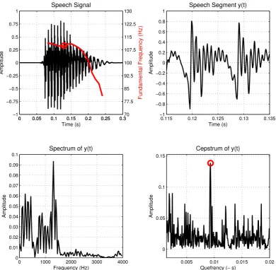
[image:25.595.126.517.105.487.2]Quefrency (∼ s)
Figure 2.2: Illustration of CepstralF0 determination. A male French speaker saying
the word “un” (œ)(upper left, black line, left axis) and the corresponding F0 curve
(upper left, red line, right axis, determined using ACF). To estimate the F0 at
as single point (red circle) we use the segment of speech around the estimation point (upper right), we then compute its Power |df t(y)| (lower left) and then the corresponding Cepstrum idf t(loge(|df t(y)|)) (lower right). The peak amplitude of
the Cepstrum occurs at time F0−1 = 0.0092 s ≈ F0 = 108.7Hz. A rectangular
window was used.
developed but work again in a time-step principal. No established methodology for choosing the window-length exists. Most popular implementations (eg. Praat [32] and Wavesurfer [295]) aside from using standard predetermined window sizes, are based on “how low”F0 is expected to be; effectively estimating a maximin window
length of a frame.
Complementary to autocorrelation based methods are the double-transform
transform of the natural logarithm of the spectrum. Because it is the inverse trans-form of a function of frequency, the cepstrum is a function of a time-like variable
[285].
Taking a step back and assuming a time-domain indext,t∈[0, T], T being the total duration of a time samplex(t), the complex spectrum frequencyX(f) for any frequencyf is the forward Fourier transformation ofx(t) [251]:
X(ω) =
Z T
0
x(t)e−ωitdt, ω = 2πf (2.3) where it can be immediately seen that the Fourier transformation is a continuous function of frequencyf, the inverse of it expressing the signal as a function of time as:
x(t) = 1 2π
Z
X(ω)eωitdω. (2.4) Continuing, the instantaneous powerP(t) and energyE of a signalx(t) are respec-tively defined as:
P(t) =x2(t) and (2.5)
E =
Z
P(t)dt =x2(t)dt where by using Eq. 2.4 (2.6)
E = 1 2π
Z
X(ω)X(−ω)dω = 1 2π
Z
|X(ω)|2dω =
Z
E(ω)dω (2.7) representing that qualitative signal energy is the accumulation of energy spectral densityE(ω). Moving to a discrete signalx[n] now, the discrete-time Fourier trans-formation of it is defined as:
X(eiω) =
∞
X
t=−∞
x[t]e−iωtdt, (2.8)
the inverse of it being defined in respect to its complex logarithm as [24]: ˆ
x[t] = 1 2π
Z π
−π
ˆ
where the complex logarithm ˆX is: ˆ
X(eiω) = log[X(eiω)]. (2.10) Based on this, one is able to then define the cepstrum of a discrete signalx[n] as:
c[n] = 1 2π
Z π
−π
log(|X(eiω)|)eiωndω, (2.11) or in a purely discretised form as: =
N−1 X
n=0
log(|
N−1 X
n=0
x[n]e−i2Nπkn|)ei
2π
Nkn, (2.12)
and recognize that during cepstral analysis the power spectrum of the original signal is treated as a signal itself. As a result instances of periodicity in that signal will be highlighted in the original signal’s cepstrum. Essentially the cepstrum’s peaks will coincide with the spacing between the signal’s harmonics (Fig. 2.2). As expected the cepstrum is a function of time orquefrency, where the quefrency approximates the period of the signal examined (ie. larger quefrencies relate to slower varying components).
One might question the complacency of the twoF0 tracking techniques; the
answer though is rather straight-forward and is known as the Wiener-Khinchin the-orem [54]. Taking Eq. 2.1 and substituting x(t) using the inverse Fourier transfor-mation, Eq. 2.1 becomes:
αf(d) =
Z ∞
−∞
x(t)x(t+d)dt = 1 2π
Z ∞
−∞
eωit|X(ω)|2dω =
Z ∞
−∞
eωitE(ω)dω
(2.13) and it therefore becomes obvious that the Fourier transformation of the energy spectral densityE(ω) (Eq. 2.7) is the autocorrelation function associated with the signal x(t). Other methods for pitch determination based on Linear Prediction
[250; 289],Least Squares Estimation [87; 217] and directHarmonic Analysis [1; 220] have also offered certain practical advantages on application-specific projects but they have failed to established themselves as generic frameworks in comparison with the two methods previously described.
usual stationary assumptions. Excluding more specialized techniques such as non-linear filtering [319], the usual counteraction is to usewindowing (orlifting [33]); an important preliminary step where we frame a segment y(t) of our signal x(t) and assume y(t) to be locally stationary. They are many different window types; three of the most common windows of sizeLare :
• the rectangular (w(n) = 1),
• the Hamming (w(n) =.54−.46cos(2πNn), L=N + 1),
• the Gaussian window (w(n) = exp(−1 2(
n σ)
2)),
the latter one being an infinite-duration window. While somewhat trivialized in the context of signal analysis windowing properties such as frame size, type and shift can have very profound effects in the performance of a pitch determination algorithm (Fig. 2.3) and subsequent feature extraction. The relation of windowing and kernel smoothing (Sect. 3.1), as it will be shown later, is all but coincidental and windowing in the sense presented above is a simple reformulation a general ”weighting” scheme in mainstream Statistics.
Complementary to this F0 estimation via the DFT is the task of
spectro-gram estimation. Without going to unnecessary details, a spectrospectro-gram is simply the concatenation of successive Fourier transformations along their frequencies. As in the case of F0, windowing in terms of segment length and window type
signif-icantly affects the resulting two-dimensional function, one of the axes being time (t) and the other frequency (f) (eg. Fig. 2.1 lower panel). We draw attention to a very interesting property of spectrograms: while spectrograms are subject to the same time distortion (See section 3.2) as every other phonetic unit of analysis, time distortion is only meaningful across their time-axis. While smearing (or leakage) can occur between successive frequency bands [24], this is not time-dependent and is usually associated with recording conditions (eg. room reverberation) and/or win-dowing. In practice, given we employ conservative choices of windowing, we assume that leakage is minimal. Therefore the frequency axis f is assumed to evolve in “equi-spaced” order with no systematic distortions present; we will reiterate these insights in section 6.2.1.
2.2
Tonal Languages
0.115 0.12 0.125 0.13 0.135 −1
−0.5 0 0.5 1
Rectangular Speech Segment y(t)
Time (s)
Amplitude
0.115 0.12 0.125 0.13 0.135 −1
−0.5 0 0.5 1
Gaussian Speech Segment y(t)
Time (s)
Amplitude
0.115 0.12 0.125 0.13 0.135 −1
−0.5 0 0.5 1
Hamming Speech Segment y(t)
Time (s)
Amplitude
0.005 0.01 0.015 0.02 0
0.05 0.1 0.15
Cepstrum of y(t)
Amplitude
Quefrency (∼ s)
0.005 0.01 0.015 0.02 0
0.05 0.1 0.15
Cepstrum of y(t)
Amplitude
Quefrency (∼ s)
0.005 0.01 0.015 0.02 0
0.05 0.1 0.15
Cepstrum of y(t)
Amplitude
[image:29.595.123.517.105.369.2]Quefrency (∼ s)
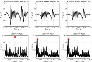
Figure 2.3: Illustration of Cepstral F0 determination employing different windows.
The peak amplitude of the Cepstrum occurs at timeF0−1= 0.0092 s≈F0 = 108.7Hz
in the case of a rectangular window (Left hand-side plots). The peak amplitude of the Cepstrum occurs at timeF0−1 = 0.0024 s≈F0 = 416.7Hz both in the case of a
Gaussian and of a Hamming window (Center and Right hand-side plots).
changes the lexical meaning of a word in a predetermined way [301]. Among tonal languages Mandarin Chinese is by far the most widely-spoken; it is spoken as a first language by approximately 900 million people [53], with considerably more being able to understand it as a second language. It is therefore of interest to try and pro-vide a pitch typology of Mandarin Chinese in a rigorous statistical way incorporating the dynamic nature of the pitch contours into that typology [111; 245]. This interest is not only philological for Indo-European languages’ speakers. Discounting the ob-vious advantage that an accurate typology will offer in automatic speech recognition and speech/prosody production algorithms [69], with the increasing interest in tonal Asian languages as second languages, potential learners could greatly benefit from an empirically derived intonation framework; second language acquisition being an increasingly active research field [140]. Phenomena such as synchronic or diachronic tonal stability, while prominent in tonal languages, are quite difficult to encapsulate in strict formal rules [100] and they are known to manifest in significant learning difficulties.
with different tones implies:
• Tone1 (m¯a 媽 “mother”) a steady high-level sound,
• Tone2 (m´a 麻 “hemp”) a mid-level ascending sound,
• Tone3 (mˇa 馬 “horse”) a low-level descending and then ascending sound,
• Tone4 (m`a 罵 “scold”) a high-level descending sound and
• Tone5 (m ˙a嗎 question particle) an unstressed sound.
This means that the rather artificial statement媽媽罵麻馬嗎 / “Does mother scold the numb horse??” is actually transliterated in Pinyin5 as: “m¯am ˙a m`a m´a mˇa m ˙a?” where without the pitch patterns shown in the diacritic markings it would be totally incomprehensible [330].
As Fujisaki recognizes though, while in tonal languages (eg. Mandarin) pitch is modulated by lexical information, para- and non-linguistic effects have significant impact to the speaker utterances [90]. In other words, to assume that the differ-ences observed in intonation pattern is only due to the words’ lexical meaning is an oversimplification. Non-lexical effects come into play. In particular by para-linguistic effects we mean contextual and semantic information that affects a user’s utterance. For example the same speaker might employ different intonation pat-terns for a formal announcement to that of a private conversation with a friend. Moreover non-linguistic effects related directly to the speaker’s physiological char-acteristics also have prominent influence in the final syllable modulation [333; 117]. AsF0 is associated with the function of the vocal cords, and like most physiological
properties of an organism this functionality is influenced by the age, health and general physical characteristics of a speaker, speaker related variation should not be neglected.
2.3
Pitch & Prosody Models
The rhythmic and intonational patterns of a language [159] are known as prosody. Prosody andF0modelling are intertwined asF0is a key component of prosody6and
this connection is even stronger in tonal languages like Mandarin Chinese. Accurate modelling of the voicing structures enables the accurate modelling of voiced speech segments thus assisting all aspects of speech related studies: synthesis, recognition, and coding [69].
5
Pinyin is the official form of the Latin alphabet transliteration of Mandarin Chinese used by the People’s Republic of China [328].
6
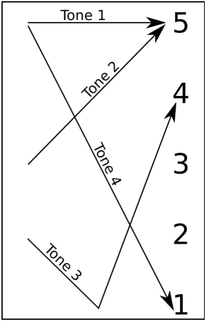
Figure 2.4: Reference tone shapes for Tones 1-4 as presented in the work of Yuen Ren Chao; Tone 5 is not represented as it lacks a general estimate, always being significantly affected by non-standardized down-drift effects. Vertical axis represents impressionistic pitch height. Somewhat generally, the
“ref-erence framework” for the analysis and synthesis of intonation patterns is ToBi [158]. As defined by its creators:“ToBi is a framework for developing community-wide conven-tions for transcribing the intona-tion and prosodic structure of spo-ken utterances in a language vari-ety”. ToBi defines five pitch accents and four boundary tones based on which it categorizes each respec-tive utterance. ToBi is effecrespec-tively a complete prosodic system; it has two important caveats. First ToBi is not a universal system. There are language-specific ToBi systems that are non-communicative to one another; this is a major shortcom-ing in its generality. In that sense its rigidity has rendered it too re-strictive to model even English va-rieties (ToBi was specifically devel-oped for the English language orig-inally) leading to the development
of IVie [103]. Secondly though it also defines a series of different break types, acting as phrasing boundaries. Break counts are very significant as physiologically a break has a resetting effect on the vocal folds’ vibrations; a qualitative description of break counts is provided in Table 2.1. This recognition of the importance of breaks high-lights an important physiological characteristic ofF0; while a continuous trajectory
is meaningful for temporal modelling, anF0trajectory is not a continuously varying
parameter along an utterance but rather a series of correlated discrete events that are realized as continuous curves.
Complementary to ToBi is the work of Taylor with the TILT model [305].
Break Type Meaning
Break 1 Normal syllable boundary. In languages like written Chinese where there is “no alphabet” but the written system corresponds directly to morphemes, this corresponds to a single character. (As syllable segments will often act as our experimental data units, B1 is equivalent to the mean value of the statistical estimates and thus not examined separately as a “dependent variable”).
Break 2 Prosodic word boundary. Syllables group together into a word, which may or may not correspond to a lexical word.
Break 3 Prosodic phrase boundary. This break is marked by an audible pause.
Break 4 Breath group boundary. The speaker inhales.
Break 5 Prosodic group boundary. A complete speech paragraph. Table 2.1: ToBi Break Annotation
effectively a continuous description of theF0 curve that is a function of the duration
Dand the amplitudeA of the intonation pattern examined. In particular: Tilt = |Arise| − |Af all|
2(|Arise|+|Af all|)
+ Drise−Df all 2(Drise+Df all)
. (2.14) The TILT model was in a way influential because it really provided an empirical and continuous representation of F0. Nevertheless in the end TILT uses three,
undoubtedly important numbers to characterize a single curve. This is not “wrong” (the popularity of TILT hinting that these three numbers are highly effective), but ultimately fails to provide a framework that can be directly expanded to account of increasing sample complexity. Additionally it does not account for speaker related information affecting an utterance nor for explicit interaction between successiveF0
curves.
This is one of the main intuitions behind the third and final “reference model” for intonation patterns: the Fujisaki model [90]. The Fujisaki model was introduced by Fujisaki and Ohno in 1997 and was extended mostly by the cooperation of Fujisaki with Mixdorff7. Similarly to the TILT model, the Fujisaki model is a quantitative model that does not use explicit labels. The basic modelling assumption behind the Fujisaki model is that the F0 contour along a sentence is the superposition of
both a slowly- and a rapidly-varying component [90]. The slowly-varying component commands the overall curvature of theF0contour along the duration of the sentence,
the rapidly-varying relates to the lexical tone. This major idea came from the way theF0production mechanism is treated: the laryngeal structure being approximated
7
by Fujisaki’s earlier work as effectively the step response function of a second-order linear system [133]. Another important theoretical break-through of the Fujisaki model was that it explicitly incorporated speaker related information or better yet uncertainty; for example it assumes that the lowerF0 attainable is a speaker related
rather than universal characteristic and that it should be treated as an unobserved random variable. The major shortcoming of the Fujisaki model actually comes from within its design: the idea of a slow-varying down-drift deterministic component is rather restrictive, despite being a reasonable norm. Especially in its original format this assumption fails to account for intonation patterns in Western languages [305]. Also in its original form the Fujisaki model advocated the use of a rigid gradient for each of the rapidly-varying components; a position where the TITL model was definitely more flexible.
A number of other prosodic frameworks have been based on these three basic ones (eg. MOMEL [135], INTSINT [196], qTA [244], etc.) but few have presented a prosodic framework that offers a universal “language-agnostic” approach. The presented work in later chapters of this thesis strives to deliver exactly that.
2.4
Linguistic Phylogenies
Following once again the view of a language as a system that interacts with its environment, the concept of linguistic Phylogenetics is not ungrounded within the general phylogenetic framework 8. Indeed in the last 15 years there has been a steady increase of papers where language development and biological speciation have been treated as quite similar [320]. Pagel in his eponymous review paper “Human language as a culturally transmitted replicator” [230] not only argues on the similarity of genes’ and languages’ evolutionary behaviour but offers an extensive catalog of analogies between biological and linguistic evolution as well.
Interestingly one might even argue that linguistic phylogenetic studies pre-ceded biological ones at least in theWestern world. While Aristotle (382-322 BC) was probably one of the first to cluster different animal species in terms of com-parative methods [10], Socrates (469-399 BC), among other philosophers, actually realized that language “changed” (or at least “decayed”) as time passed [49]. The reason for this observation was relatively simple: Homer’s (∼8th century BC) writ-ings while revered as accounts of heroic tradition, they were already at least 350 years old at the time of Socrates. People simply realized that Achilles did not speak like them. One of the first to formulate an actual “connection” though between Linguistics and Biology was Gottfried W. Leibniz (1646-1716)9. Leibniz advocated
8
See section 3.5 for a short introduction in Phylogenetics.
9The reader will note a significant chronological gap. Aside the obvious need for significant
the idea ofNatura non facit saltus(“nature does not make jumps”), gradual change. In addition to that he also advocated the ideas of Monadology: fundamental imma-terial units that are eternal were “the grounds of all corporeal phenomena” [195]. Those ideas proved fundamental both in Biology and Linguistics. Therefore it is not surprising that the father of modern Biology, Charles R. Darwin (1809-1882) also made similar assertions regarding language in his landmark workThe Origins of Species. Leaving historical remarks aside, the seminal paper of Cavalli-Sforza et al. [52] changed the way linguistic and genetic information are combined within a single analysis framework in modern times. There the authors focused on the reconstruction of a human phylogeny based on maximum parsimony 10 principles but importantly, after pooling genetic data geographically in order to account for heterogeneity, if heterogeneity persisted, they added an “ethnolinguistic criterion of classification”. That allowed the synchronous derivation of a genetic and a linguistic phylogeny that displayed significant overlap and emphasized that the two fields not only could share methods but also results.
Up until relatively recently maximum parsimony trees [321; 107] and com-parative methods[320] stood as the state-of-the-art in Linguistic Phylogenetics. And while comparative methods were already employed rather broadly within the con-text of glottochronology [105] the question of computational reconstruction of pro-tolanguages started to emerge [227; 268]. Importantly people began to incorporate the phonetic principals in their tree reconstructions. Research came to the realiza-tion that exactly because language was just a human-bounded characteristic, direct analogies with generic Phylogenetics were not only possible, but actually strength-ening the theoretical framework used. Language acquisition being associated with children (founder effects), parallel development of characteristics being not as un-common as originally thought (convergent evolution), insertion-deletion-reversals being usual “units of changes” (the same operations being used in the changes of genetic code) showed that even qualitative linguistic phenomena could be en-capsulated within a phylogenetic framework. Evidently the inherent problems of Phylogenetics such as having (2N−3)!!11 rooted-trees for N leaves and being pre-sented with a relatively small amount of data compared to the number of candidate trees [138] did remain, but linguists were nevertheless able to validate a very cru-cial insight from sociolinguistics: “while most linguistic structures can be borrowed between closely related dialects, natively acquired sound systems and inflections are resistant to change later in life” [268]. That meant that essentially a sound system was resistant to change and therefore presented a “good” character for phylogenetic
the Biblical story of the Tower of Babel made the question of linguistic phylogenies somewhat heretic.
10See Sect. 3.5.2 for an overview of tree reconstruction methodologies.
11
The double or odd factorial where (2k−1)!! =(22kkk)!! or more generally: (2k−1)!! = Π
k
studies. Insights like the positive correlation between rates of change and speaker population size [12] and the coherence of rule-based changes [221; 39] were estab-lished. Importantly almost all these techniques rely on binary features [73] or at a best case scenario multi-state ones [231; 106]. While computational linguists rec-ognized the importance of phoneme sequences [39; 38] they do not act on premises of continuous data. As it will be shown in following chapters, the current work is not qualitatively comparable with state-of-the-art multi-state implementations [38] where the number of available training data is significantly larger. In addition, even excluding training sample size issues, the current methodology also acts almost ag-nostically in relation with semantic information by only using phonetic information. Undoubtedly the choice of discarding semantic information is a strong (yet not un-common [105; 231]) assumption from a linguistic point of view but it presents itself as a definite progress in the phonetic literature because up until now comparative methods focused on scalar characteristics only.
As a final note we draw attention to the notion of themolecular clock of a biological phylogeny [165] and its significance in a linguistic phylogeny. As Gray et al. note, absolute dates in Linguistics are notoriously hard to get [106]. Disregarding the issues that relate to tree uncertainty and lack of concrete evidence, this difficulty is rooted with the quite restrictive assumption of (in this case) lexical clock (or a
glottoclock). Exactly because one asserts that changes “occur in a more-or-less clocklike fashion, so that divergence between sequences should be proportional to the evolutionary time between the two sequences” [165], this assumption is hard to evaluate experimentally [105; 76]. Nevertheless we need this assumption for standardMaximum Likelihood methodology to be applicable. It would be therefore interesting to explore a possible application of methodologies that act under the assumption of a non-universal time- continuum. The current work does explore this in terms of the observational time on the phylogeny’s leaves but leaves the question of actual phylogenetic time (and its potential time-distortion) for future work.
2.5
Datasets
The current work employs two functional datasets. Both of them were made avail-able to the author by his respective collaborators.
2.5.1 Sinica Mandarin Chinese Continuous Speech Prosody Cor-pora (COSPRO)
0 0.5 1 50
100 150 200 250 300 350
Hz
t Tone1
0 0.5 1
50 100 150 200 250 300 350
Hz
t Tone2
0 0.5 1
50 100 150 200 250 300 350
Hz
t Tone 3
0 0.5 1
50 100 150 200 250 300 350
Hz
t Tone4
0 0.5 1
50 100 150 200 250 300 350
Hz
t Tone5
[image:36.595.143.501.106.319.2]M01 M02 F01 F02 F03
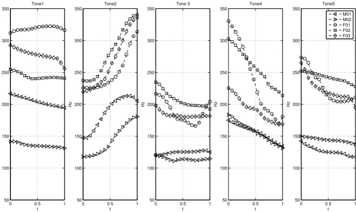
Figure 2.5: Tone realization in 5 speakers from the COSPRO-1 dataset.
the phonetically balanced speech database consists of recordings of Taiwanese Man-darin read speech. The COSPRO-1 recordings themselves were collected in 1994. COSPRO-1 was designed to specifically include all possible syllable combinations in Mandarin based on the most frequently used 2- to 4-syllable lexical words. Addi-tionally it incorporates all the possible tonal combinations and concatenations. It therefore offers a high quality speech corpus that, in theory at least, encapsulates all the prosodic effects that might be of acoustic interest.
After pre-processing and annotation, the recorded utterances, having a me-dian length of 20 syllables, resulted in a total of 54707 fundamental frequency curves. Each F0 curve corresponds to the rhyme portion of one syllable. The three female
and two male participants were native Taiwanese Mandarin speakers. Using the in-house developed speech processing software package COSPRO toolkit [311; 312], the fundamental frequency (F0) of each rhyme utterance was extracted at 10ms
in-tervals, a duration under which the speech waveform can be regarded as a stationary signal [131]. Associated with the recordings were characterizations of tone, rhyme, adjacent consonants as well as speech break or pause. Importantly the presented corpus is a real language corpus and not just a series of nonsensical phonation pat-terns and thus while designed to include all tonal combinations, it still has semantic meaning.
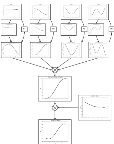
Effects Values Meaning Notation-mark
Fixed effects
previous tone 0:5 Tone of previous syllable, 0 no previous tone present
tnprevious
current tone 1:5 Tone of syllable tncurrent
following tone 0:5 Tone of following syllable, 0 no following tone present
tnnext
previous conso-nant
0:3 0 is voiceless, 1 is voiced, 2 not present, 3 sil/short pause
cnprevious
next consonant 0:3 0 is voiceless, 1 is voiced, 2 not present, 3 sil/short pause
cnnext
B2 linear Position of the B2 index break in sentence
B2 B3 linear Position of the B3 index break
in sentence
B3 B4 linear Position of the B4 index break
in sentence
B4 B5 linear Position of the B5 index break
in sentence
B5 Sex 0:1 1 for male, 0 for female Sex
Duration linear 10s of ms Duration
rhyme type 1:37 Rhyme of syllable rhymet
Random Effects
[image:37.595.135.506.113.465.2]Speaker N(0,σspeaker2 ) Speaker Effect SpkrID Sentence N(0,σsentence2 ) Sentence Effect Sentence Table 2.2: Covariates examined in relation toF0production in Taiwanese Mandarin.
Tone variables in a 5-point scale representing tonal characterization, 5 indicating a toneless syllable, with 0 representing the fact that no rhyme precedes the current one (such as at the sentence start). Reference tone trajectories are shown in Fig. 2.4.
5 speakers.
2.5.2 Oxford Romance Language Dataset
three (3) Portuguese speakers. We were unable to have records for all 10 digits from all speakers, this finally resulting in a sample of 219 recordings. The sources of the recordings were either collected from freely available recordings from language training websites or standardized recording made by university students.
Language Number of Speakers (F/M) French 7 (4/3)
Italian 5 (3/2) American Spanish 5 (3/2) Iberian Spanish 5 (4/1) Portuguese 3 (2/1)
Table 2.3: Speaker-related information in the Romance languages sample. Numbers in parentheses show how many female and male speakers are available.
An important caveat regarding this dataset is it is “real world”. This trasts with the COSPRO dataset that was recorded under phonetic laboratory con-ditions. The Romance language dataset consisted of recordings people made under non-laboratory settings (eg. classes, offices). It is also heterogeneous in terms of bit-rate sampling, duration and even format. As such before any phonetic or statistical analysis took place, all data were converted in *.wav files of 16Khz. This clearly un-dermines the quality of the recordings compared to the ones acquired by COSPRO but these conversions were deemed essential to ensure sample homogeneity. Fig. 2.1 shows a typical waveform reading.
Italian
American Spanish
Iberian Spanish Portuguese
French
Romance Language Unrooted Phylogeny
Chapter 3
Statistical Techniques for
Functional Data Analysis
Functional Data Analysis (FDA) defines a framework where the fundamental units of analysis are functions. The dataset are assumed to hold observations from an underlying smoothly varying stochastic process. FDA application works in both a parametric and a non-parametric setting. Using a parametric framework one usually assumes that the underlaying process is a member of a specific class of functions, eg. Gaussian [122], Dirichlet [236], Poisson [147] or some other generalization of point-processes (eg. Cox processes) [40; 26]. Under a non-parametric framework one directly usually utilizes a spline- [254] or a wavelet-based [115] representation of the data. Nevertheless irrespective of the framework used as stated by Valder-rama: “approximations to FDA have been done from two main ways: by extending multivariate techniques from vectors to curves and by descending from stochastic processes to real world” [317].
In particular if one considers a smooth1 functionY(t),t∈T, ifE{Y(t)}2 <
∞ and E{R
Y2(t)dt} < ∞, Y is said to be squared integrable in the domain T. Additionally if one assumes that the instances of functionY, ie. a functional dataset
Yij, define a vector space inL2[0,1] that space has a vector space basis spanning it.
A smooth random processesY can be defined to have a mean function:
µY(t) =E[Y(t)] (3.1)
1Contrary to more rigorous definitions of smoothness, here smoothness in relation to a dataset’s