Phonons in disordered harmonic lattices

(1)

University of Warwick institutional repository: http://go.warwick.ac.uk/wrap

A Thesis Submitted for the Degree of PhD at the University of Warwick

http://go.warwick.ac.uk/wrap/57512

This thesis is made available online and is protected by original copyright.

Please scroll down to view the document itself.

(2)

Phonons in Disordered Harmonic Lattices

by

Sebastian Pinski

Thesis

Submitted to the University of Warwick

for the degree of

Doctor of Philosophy

Physics Department

(3)

Acronyms

1D one-dimension. vi, 3, 8, 9, 11, 20, 22, 26, 27, 30–32, 34, 61, 64, 76, 81, 107, 118

2D two-dimensions. 8, 9, 81, 107

3D three-dimensions. vi, 3, 9, 11, 16, 20, 30, 31, 34, 35, 37, 46, 55, 106, 118

AM Anderson model. 7, 55–57, 78, 87, 106, 107, 117, 119

BP ‘boson-peak’. vii, 3, 48–51, 53, 54, 80, 85–87, 90–92, 96, 97, 119

CPA coherent potential approximation. 34, 41–43, 45–48, 50, 52, 80, 119

DOS density of states. vi, 7, 8, 14, 31, 33, 43–48, 58, 99, 106, 119

FSS finite size scaling. vi, 58, 64, 68, 70, 71, 74–79, 109, 120–124

gIPR generalised inverse participation ratio. vi, 93, 99, 102, 104, 107

GOE Gaussian orthogonal ensemble. 50, 85, 86, 88, 89, 92, 119

IPR inverse participation ratio. 102

LDT localisation-delocalisation transition. vi, 3, 8, 11, 33, 41, 48, 51, 55, 56, 58–60,

66, 72, 78, 79, 84–87, 93, 94, 96, 99, 102, 105, 106, 109, 116–119

MFA multi-fractal analysis. 93, 99, 117, 119

MIT metal-insulator transition. 8–10, 80, 102, 112, 116, 119

NLσM non-linear sigma model. 8, 106

(7)

PR participation ratio. 14, 21–29, 78, 93–99

PTD Porter-Thomas distribution. vii, 85–90, 92, 96

RMT random matrix theory. 85, 86

TMM transfer-matrix method. vi, 27, 30, 32, 58, 61, 66, 67, 78, 81, 82, 96, 99, 119

VDOS vibrational density of states. 21–25, 27–29, 33, 34, 40–43, 45, 47–50, 52,

(8)

List of Tables

6.1 For orders of expansionnr0,nr1,ni,mrandmifrom finite size scaling,

critical parametersωc orω2c andν, with the minimisedχ2 value, the

degrees of freedom µ and the resulting goodness-of-fit parameter Γq

for pure mass and pure spring constant disorders. . . 78

A.1 Critical parameters for lowest stable fits and higher order stability

testing fits, from finite size scaling (in the ω2 domain) of reduced

localisation lengths of mass disordered crystals with disorder

distri-bution widths ∆m= 1.2,4 and 9. . . 121

testing fits, from finite size scaling (in theω domain) of reduced

local-isation lengths of mass disordered crystals with disorder distribution

widths ∆m= 1.2,4 and 9. . . 122

testing fits, from finite size scaling (in theω2 domain) of reduced

lo-calisation lengths of spring constant disordered crystals with disorder

distribution widths ∆k= 1,7 and 10. . . 123

testing fits, from finite size scaling (in the ω domain) of reduced

lo-calisation lengths of spring constant disordered crystals with disorder

(9)

List of Figures

1.1 Image of a partially fried egg placed on an iPad to satirise the iPad

heat controversy. . . 2

2.1 Thermal conductivity of Germanium as a function of percentage

ran-dom substitution of Silicon. . . 5

2.2 Schematic electronic density of states and phase diagram as functions

of potential disorder. . . 7

2.3 Schematic example showing the behaviour of scaling function β for

dimensions d= 1,2 and 3 . . . 9

3.1 Diagram illustrating the difference in sparsity of dynamical matrices

for a periodic three-dimensional cubic systems of width L= 5 and 15. 16

4.1 Participation ratios and vibrational density of states for a one-dimensional

binary disordered chain of lengthL= 1000 . . . 23

4.2 Vibrational density of states, participation ratios, effective dispersion

and normal modes of one-dimensional Fibonacci chains of lengthL=

1000 and Fibonacci numbers Fn of n= 8–12 . . . 25

4.3 Vibrational density of states, participation ratios and effective

dis-persion for one-dimensional chain of length L = 1000 with box

dis-tributed mass disorder . . . 28

4.4 Vibrational density of states, participation ratios and effective

dis-persion for one-dimensional chain of length L = 1000 with box

dis-tributed spring constant disorder . . . 29

4.5 Localisation lengths of a one-dimensional chain with box distributed

mass disorder plotted as functions of frequency and disorder . . . 30

4.6 Localisation lengths of a one-dimensional chain with box distributed

(10)

4.7 Localisation lengths as a function of frequency for phonons in a one

dimensional chain for a range of uniform box distributed pure mass

and pure spring constant disorders . . . 32

5.1 Diagram to demonstrate physical interpretation of three-dimensional

periodic boundary conditions . . . 37

5.2 Examples of normal modes in a three-dimensional box of size L3 =

703 with mass disorder for possible extended, critical and localised

states . . . 38

5.3 Examples of normal modes in a three-dimensional box of size L3 =

703 with spring constant disorder for possible extended, critical and

localised states . . . 39

5.4 Vibrational density of states obtained from numerical

diagonalisa-tion and coherent potential approximadiagonalisa-tion studies for both mass and

spring constant disorders . . . 42

5.5 Reduced vibrational density of states as a function of frequency for

both pure mass and spring constant box distributed disorders . . . . 49

5.6 Boson peak trajectories obtained from (both numerical

diagonalisa-tion and coherent potential approximadiagonalisa-tion) reduced vibradiagonalisa-tional

den-sity of states . . . 52

5.7 Vibrational eigenstates for positions around the mass disordered

bo-son peak trajectory for system sizeL3 = 703 . . . 53

5.8 Vibrational eigenstates for positions around the spring constant

dis-ordered boson peak trajectory for system size L3 _{= 70}3 _{. . . .} ₅₄

6.1 Examples of previously published electronic phase diagrams for box

distributed potential disorders . . . 58

6.2 Phase diagram conversion schematic from potential disordered

elec-tronic phase diagram to mass disordered phonon phase diagram . . . 59

6.3 Reduced localisation lengths (as a function of squared frequency) and

finite size scaling functions/correlation lengths with varying

quasi-one-dimensional system sizes for box distributed mass disorder widths

∆m= 1.2,4 and 9 . . . 64

6.4 Reduced localisation lengths (as a function of squared frequency) and

finite size scaling functions/correlation lengths with varying

quasi-one-dimensional system sizes for box distributed spring constant

(11)

6.5 Reduced localisation lengths with analogous re-entrant behaviour in

the negative squared frequency domain for box distributed mass

dis-order width ∆m= 9 . . . 67

6.6 Distributions of critical parameters from Monte Carlo error analysis

to obtain accurate unsymmetric error bars for critical parameters of the localisation-delocalisation transition for box distributed mass

disorder width ∆m= 1.2 . . . 72

6.7 Distributions of critical parameters from Monte Carlo error analysis

to obtain accurate unsymmetric error bars for critical parameter of

localisation-delocalisation transition for box distributed spring

con-stant disorder width ∆k= 1 . . . 73

6.8 Comparison of scaling for both frequency and squared frequency

de-pendant variables with synthetic reduced localisation lengths . . . . 74

6.9 Reduced localisation lengths (as a function of frequency) and finite

size scaling functions/correlation lengths with varying quasi-one-dimensional

system sizes for box distributed mass disorder widths ∆k= 1.2,4 and 9 76

6.10 Reduced localisation lengths (as a function of frequency) and finite size scaling functions/correlation lengths with varying quasi-one-dimensional

system sizes for box distributed spring constant disorder widths ∆k=

1,7 and 10 . . . 77

6.11 All twelve critical exponents from both frequency and squared

fre-quency localisation-delocalisation transitions plotted with estimated

errors and the overall weighted average . . . 79

6.12 Phase diagram of localisation-delocalisation transitions for phonons

with applied box distributed mass disorder . . . 80

with applied box distributed spring constant disorder . . . 81

6.14 Electronic hopping disorder phase diagram for comparison to spring

constant disorder phase diagram . . . 82

with applied box distributed spring constant disorder truncated so

that all spring constants |k|>10−4 . . . 83

7.1 Histograms of eigenvector displacements and difference with respect

to the Porter-Thomas distribution for a range of frequencies in a three-dimensional system with the inclusion of uniform box distributed

(12)

7.2 Histograms of eigenvector displacements and difference with respect

to the Porter-Thomas distribution for a range of frequencies in a three-dimensional system with the inclusion of uniform box distributed

spring constant disorder of width ∆k= 1 . . . 89

7.3 Minima of deviations from Porter-Thomas distribution as a function

of frequency for multiple disorders of both mass and spring constant

type . . . 91

8.1 Scatter plot of participation ratio versus squared frequency for all

normal modes of 50 disorder realisations of mass and spring constant

disorders ∆m= 1.5 and ∆k= 1 in a three-dimensional system of size

L3 = 153 . . . 95

8.2 Participation ratios averaged over 50 realisations of box distributed

mass or spring constant disorder as a function of squared frequency

for system sizeL3 = 153 . . . 97

8.3 Running average over 100 frequency values on roughly 170,000

par-ticipation ratios per system size L3 = 53,103 and 153 in search of

a localisation-delocalisation transition for mass and spring constant

disorders ∆m= 1.5 and ∆k= 1 . . . 98

8.4 Romanesco broccoli is a natural self-affine structure whose

cross-section resembles the Koch curve, a fractal with fractal dimension

Df = 1.2619. . . 100

8.5 Schematic example of construction of the Mandelbrot-Given fractal . 101

8.6 Schematic example of the multifractal singularity spectrum with known

features labelled appropriately . . . 104

8.7 Example normal modes at criticality for mass disorder ∆m= 1.2 in a

three-dimensional cubic system of size L3 = 903 and spring constant

disorder of ∆k= 10 in a system of sizeL3 = 1003 . . . 110

8.8 Example linear fits to obtain mass exponentsτens(q) andαqfor integer

q values for mass disorder ∆m= 1.2 . . . 111

8.9 Example linear fits to obtain fq for ∆m = 1.2 to construct the

sin-gularity spectrum . . . 112

8.10 Numerical singularity spectrum f(α) for mass disorder ∆m= 1.2 . . 113

8.11 Numerical singularity spectrum f(α) for spring constant disorder

∆k= 1 . . . 114

8.12 Numerical singularity spectrum f(α) for spring constant disorder

(13)

8.13 Numerical singularity spectrum f(α) for mass disorder ∆m = 1.2

and spring constant disorder ∆k = 10 in comparison with a high

precision electronic singularity spectrum obtained numerically at the

(14)

Acknowledgments

First and foremost I dedicate this thesis to my life partner - Jenny Gordon. Without

her continuing support I would never have gotten to this stage; not only in my

research career, but life in general. I’ve been blessed by her presence ever since we

met and hope that she can keep being my guiding light for however long I shall live.

I am forever indebted to my supervisor, Prof. Rudolf A. R¨omer for accepting

me for a research degree, and thank him not only for his invaluable input to my

work but also for the friendly and creative atmosphere he has developed within our

modestly sized research group. I also thank Dr. Alberto Rodriguez-Gonzales for

being a close friend during my first years at Warwick University, and an ocean of

knowledge that I tapped into so often. I could not have done this without you both.

Other notable mentions go to other Disordered Quantum Systems group

members throughout the years, in no particular order: Dr. Andrea Fischer, Dr.

Louella Vasquez, Dr. Emilio Jimenez, Jack Heal, Andrew Goldsborough, Clara

Gonz´alez-Santander, Carlos Paez and numerous other visitors. I thank you all for

being like family to me.

I extend my gratitude to the Physics Department at the University of

War-wick and the EPSRC for funding and providing me with some fantastic opportunities

to present this work at numerous international conferences and warmly acknowledge

the additional funds granted to me by the IOP (C R Barber Trust and the Research

Student Conference Fund) and the University of Warwick American Study and

(15)

Declarations

I hereby declare that this thesis entitled “Phonons in Disordered Harmonic Lattices”

is an original work and has not been submitted for a degree, diploma or other

qualification at any other University or degree granting institution. Chapters 1 to

3 provide information gathered from literature as referenced in the text, whereas

chapters 4 to 8 are based on the following publications:

• “Study of the localization-delocalization transition for phonons via transfer

matrix method techniques”, S. Pinski and R. A. Roemer, J. Phys. Conf. Ser.

286, 012025 (2011);

• “Anderson universality in a model of disordered phonons”, S. Pinski, W.

Schir-macher and R. A. Roemer, Europhys. Lett.97, 16007 (2012);

• “Localization-delocalization transition for disordered cubic harmonic lattices”,

S. Pinski, W. Schirmacher, T. E. Whall, and R. A. Roemer, J. Phys.: Condens.

Matter. 24, 405401 (2012);

• “Universal multifractal behaviour for phonons and electrons at the Anderson

transition”, S. Pinski, A. Rodriguez, W. Schirmacher, and R. A. Roemer, AIP

Conf. Proc.1506, 62 (2012).

(16)

Abstract

This work explores the nature of the normal modes of vibration for harmonic

lattices with the inclusion of disorder in one-dimension (1D) and three-dimensions

(3D). The model systems can be visualised as a ‘ball’ and ‘spring’ model in simple

cubic configuration, and the disorder is applied to the magnitudes of the masses, or

the force constants of the interatomic ‘springs’ in the system.

With the analogous nature between the electronic tight binding

Hamilto-nian for potential disordered electronic systems and the isotropic Born model for

phonons in mass disordered lattices we analyse in detail a transformation between

the normal modes of vibration throughout a mass disordered harmonic lattice and

the electron wave function of the tight-binding Hamiltonian. The transformation

is applied to density of states (DOS) calculations and is also particularly useful for

determining the phase diagrams for the phonon localisation-delocalisation

transi-tion (LDT). The LDT phase boundary for the spring constant disordered system is

obtained with good resolution and the mass disordered phase boundary is verified

with high precision transfer-matrix method (TMM) results. High accuracy critical

parameters are obtained for three transitions for each type of disorder by finite size

scaling (FSS), and consequently the critical exponent that characterises the

transi-tion is found as ν = 1.550+0₋₀._.020₀₁₇ which indicates that the transition is of the same

orthogonal universality class as the electronic Anderson transition.

With multifractal analysis of the generalised inverse participation ratio (gIPR)

for the critical transition frequency states at spring constant disorder width ∆k= 10

and mass disorder width ∆m= 1.2 we confirm that the singularity spectrum is the

(17)

considered to be universal.

We further investigate the nature of the modes throughout the spectrum of

the disordered systems with vibrational eigenstate statistics. We find deviations of

the vibrational displacement fluctuations away from the Porter-Thomas distribution

(PTD) and show that the deviations are within the vicinity of the so called

(18)

Chapter 1

Introduction

The miniaturisation of electronic devices has almost become a necessity in recent years. Manufacturers are not only expected to increase the specifications of their

products, but also decrease the form factor with every iteration of the device. The

challenges involved in the field of microelectronics are unprecedented and complica-tions arise at every step of the development process. One of the more demanding

aspects of this field is thermal management [1]. With reducing form factors, there

is little space available for bulky fans and heat sinks, prompting the development of new and innovative materials to convert and channel heat away from core

com-ponents. Sometimes this undertaking will go awry with a massive media backlash.

After the release of the ‘new iPad’ on 16thMarch 2012, the Apple product was

criti-cised in a consumer report for the ability to achieve a 47◦C operating temperature1

initiating a series of satirical images posted by technology bloggers, the most

no-table being a photograph of an egg supposedly frying on an iPad in Fig. 1.1. In most cases the newly developed materials are integrated within the electronic

cir-cuits and acquire more than just the role of thermal management. Most notable are

thermoelectric materials [2] that can generate power from a temperature differen-tial. The recent resurgence in this field has led to developments in both theory and

advanced fabrication in an attempt to increase the thermoelectric figure of merit [3],

the measure governs the efficiency of power conversion. It is defined as

ZT = σS

2_T

κe+κph

, (1.1)

where S is the Seebeck coefficient, T is the temperature, σ is the electrical

con-ductivity, κe and κph are the thermal conductivities due to electrons and phonons,

(19)

[image:19.595.201.440.106.347.2]

Figure 1.1: Image of a partially fried egg placed on an iPad by famous technology blogger Robert Scoble who was satirising the iPad heat controversy via his Instagram

account (http://statigr.am/p/151628232280579401_70).

respectively. Most methods proposed to improve the figure of merit ZT attempt

to limit the phonon propagation whilst not significantly deteriorating the electronic

transport in the system [4].

Currently two different research approaches are taken when producing

ther-moelectric materials [5]. The first approach is to develop new generations of bulk

materials that contain heavy-ion species with large vibrational amplitudes that pro-vide phonon scattering centres [6, 7]. The other is based on reducing the

dimen-sionality of the system whilst including either nanoscale constituents to confine the phonons [8] or internal interfaces arranged such that the thermal conductivity is

reduced more than electrical conductivity [9, 10]. The manufacturing techniques

have advanced in recent years, yielding the ability to produce these material, but the theoretical understanding of phonon transport must now go beyond the

macro-scopic level. We are now entering a regime where the phonons interacting with

nano-engineered structures needs to be understood at a microscopic level in order to progress in the field.

Comparatively less attention has been given to thermal transport, than to

electrical conductivity research. Since the discovery of electricity, research has

(20)

or-ders of magnitude. Thermal conductivity in solids at room temperature spans only

four [2], yet the history of thermal transport goes back to primitive humankind, far beyond that of electrical conductivity. In this thesis I investigate the effect of

disorder on vibrational modes in solids to increase understanding of the underlying

heat transport processes for a large range of frequencies. In Chap. 4, 1D systems are studied and in Chaps. 5-8 3D systems are studied where features such as the BP

(21)

Chapter 2

Theory

2.1 Heat Transport and the Effects of Disorder

Phonons are quantised travelling elastic waves associated with the displacement of ions from their equilibrium lattice positions. Acoustic phonons are the predominant

carriers of heat in any temperature regime (for electrical insulators) due to their

large group velocity compared to that of optical phonons [11]. With lowering the lattice temperature of the sample, the wavelength (and mean free path) of a phonon

increases but reaches a maximum limiting value of 2L (L being the length of the

sample), as this is the lowest possible normal mode of the system.

Perfect crystalline lattices would exhibit the lowest possible mode of the

system and in effect be a perfect thermal conductor of phonons. In nature impurities

within the medium such as grain boundaries, impurity atoms, structural defects, vacancies and dislocations (anything that changes the bond stiffness/strength of

adjacent lattice sites) cause the phonon thermal conductivityκph to reduce. This is

good evidence that impurities have the largest effect onκphat low temperatures [11].

The first theoretical studies on a single ‘light’ impurity within a linear lattice

were performed by Lifshitz et al. [12]. They found a high frequency mode that corresponded to the single light impurity moving back and fourth erratically within

a cage of heavy particles, a localised phonon.

The thermal conductivity of a bulk crystalline solid according to Debye is expressed as [13, 14]

κph(T) = kB

2π2_ν

kBT

~

3Z θD/T

0

τ(x, T) x

4_ex

(ex₋₁₎2dx, (2.1)

(22)

[image:22.595.207.436.106.349.2]

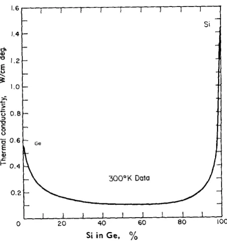
Figure 2.1: Thermal conductivity of Germanium as a function of percentage random substitution of Silicon taken from Ref. [16].

of sound in the solid, θD is the Debye temperature. The variable x = ~ω/kBT is

best described as a frequency (ω) dependant quantity,τ is the total relaxation time

of the phonons. By assuming that all scattering processes are independent of each

other, Mathiessen’s rule [7, 13] can be used to express the relaxation time as

1

τ =

1

τU

+ 1

τN

+ 1

τb

+ 1

τp

. (2.2)

HereτUandτN represent the relaxation times due to umklapp and normal processes,

respectively. These scattering types are predominately due to phonon-phonon

inter-actions and at low temperatures phophonon scattering rates are close to

non-existent, therefore we take these relaxation times to be infinite [15]. The remaining

contributions to the overall relaxation time come from boundary and particle (τb

andτp) scattering and by increasing these rates, the associated relaxation times will

reduce proportionately. This effectively reduces the overall relaxation time of the phonons and the thermal conductivity in Eqn. (2.1).

From Fig. 2.1 we see experimental evidence that with random substitution

(23)

random doping level of 50%. In order to achieve desired thermal properties in

disordered materials, where the thermal conductivity is governed by boundary and particle scattering, we must understand the characteristics of the underlying phonon

modes and all mechanisms that affect them.

2.2 Anderson Localisation

Philip Warren Anderson’s original paper [17] entitled “Absence of diffusion in certain

random lattices” saw him jointly lay claim to The Nobel Prize in Physics (1977). He shared the prize with Sir Nevill Francis Mott and John Hasbrouck van Vleck “for

their fundamental theoretical investigations of the electronic structure of magnetic

and disordered systems”. Not only did he receive one of the greatest accolades in Physics for this work, but he unleashed a major worldwide research field that even

now, 54 years later, is still very much active. Anderson theorised that with the

introduction of tiny modifications to a lattice, such as the introduction of impurities or defects, an electron that would normally move freely inside the solid no longer

diffuses on the defects as expected but can be completely stopped. In a recent press

release, Philippe Bouyer, an experimentalist in the field of Anderson localisation of matter waves [18] described an analogy of the phenomena as:

“On a macroscopic scale, [Anderson localisation] would be like saying

that a few blades of grass scattered haphazardly over a golf course could

completely stop a full-speed golf ball in its tracks.”

The majority of the research on Anderson localisation has been conducted in

the field of electron transport, although it is now known to extend to classical waves and many varying experimental realisations. Nonetheless, the following theory will

be presented in the framework of the original electronic theory [19, 20].

2.2.1 Theoretical Background of Anderson Localisation

In Anderson’s original work [17], it was stated that “the eigenfunctions [of the

electrons] are localised if the ‘strength’ of the disorder exceeds some definite value”.

Only later was it found by Mott [21] (and almost simultaneously Ziman [22]) that the transition also depends on the energy (spectral variable) of the electrons. Hence they

theorised that the spectrum is divided by amobility edge into regions where all states

(24)

(a) (b)

Figure 2.2: (a) Illustration of the electronic DOS as a function of electronic energy

E and disorder strength W adapted from Ref. [24] and (b) phase diagram between

extended and localised states adapted from Ref. [25].

of a phase transition is accepted the critical temperature for given scenarios is not

analytically know and remains difficult to calculate.

The Anderson model (AM) neglects the effects of interactions such as the electron-electron and electron-phonon interactions and is only reasonable in a regime

where all scattering is elastic (∼10K) and electrons are taken to be spinless

parti-cles. In most cases the AM involves solving the Schr¨odinger equation using a tight

binding approximation with diagonal disorder. The diagonal disorder is applied to

the diagonal terms within the Hamiltonian, which are linked to the potential at each lattice site. The Hamiltonian is of the form

H=X

i

i|iihi|+tij

X

i6=j

|iihj| (2.3)

wherei is the potential at lattice site i and tij is the hopping integral from site i

toj. In the case of potential disorder, tij is constant and set to unity.

The disorder is introduced into the onsite potentials such thati ∈

−W₂ ,W₂ ,

whereW is known as the ‘strength’ of the disorder and is usually symmetric around

= 0. As an illustration, we show the effect on the electronic DOS and the mobility

edges for increased disorder in Fig. 2.2. We can see that when the trajectory of the

mobility edges from Fig. 2.2(a) are plotted as a function of disorder strengthW we

obtain the phase diagram in Fig. 2.2(b) which is symmetric around E = 0. Most

(25)

phase boundary as not only is there a LDT but the disorder required for a

metal-insulator transition (MIT) can also be studied. It is assumed that when all electrons

withE= 0 are localised, that the system has experienced a MIT. The exact disorder

strength required for an MIT is of significant interest, where the current accepted

value is Wc ≈ 16.5 without a magnetic field. It is also favourable to work in this

region of the phase diagram as the DOS (as seen in Fig. 2.2(a)) is roughly constant

or flat. This is advantageous when working with localisation properties as it has

been shown to be more difficult to work in regions of fluctuating DOS [26].

2.2.2 Universality Classes, Renormalisation Group Theory and Scal-ing Theory

Renormalisation group theory is a tool to investigate the changes in a system when observed at varying length scales [27]. As the scale changes, it is as if the ‘magnifying

power’ set upon the system is being altered. In these renormalisable theories [28,29], the system at one scale will generally be seen to consist of ‘self-similar’ copies of itself,

when viewed at a smaller scale. The aim is to understand the behaviour of properties

in the system as a function of the system size or of other scale variables [29]. Let us consider an observable of a physical system undergoing a

renormali-sation group transformation. The magnitude of the observable as the length scale

of the system goes from small to large may be (a) always increasing, (b) always decreasing or (c) other, and these observables would be described as (a) relevant,

(b) irrelevant and (c) marginal, respectively [30]. A relevant operator is needed

to describe the macroscopic behaviour of the system. Irrelevant operators account for other systematic changes to the observable that occur in finite sized systems

and have lesser influence when approaching the thermodynamic limit. Marginal

observables may or may not need to be taken into account depending on the suc-cess of using only relevant and irrelevant variables. It is generally accepted that

most observables are of the irrelevant type, and therefore the macroscopic physics

is dominated by only a few relevant observables in most systems.

After Anderson’s original paper [17], the localisation problem was

reformu-lated in terms of renormalisation group theory [31] and the non-linear sigma model

(NLσM) [32], before finally establishing that the MIT is a second order phase

tran-sition. Within a few years, in a very similar manner, John et al. [33] described the

transition from extended to localised modes in an elastic medium using the NLσM.

They found that for phonons in a disordered system, all finite frequency modes in

1D and two-dimensions (2D) are localised, and in dimensions d > 2 there exists a

(26)

Figure 2.3: Schematic diagram of the scaling functionβ for dimensionsd= 1,2 and

3. β describes with what exponent the average conductance g grows with system

sizeL. We see that the transition occurs when d= 3 asβ can be both positive and

negative.

In the one-parameter electronic scaling theory [29] the conductanceg(L) of

electrons was taken to be the only scaling variable. It was rightly pointed out

that the DC conductivity vanishes in the localised regime and at absolute zero

temperature it is no longer a useful quantity for the description of transport through

finite sized systems [34]. The assumption was made that the quantity β = _dd_ln(ln(_Lg)₎

in a ‘hypercube’ of volumeLddepends solely ong(L) and not separately on system

sizeL, energy or disorder. The qualitative behaviour of the dependance of β upon

g is given in Fig. 2.3 and was estimated by interpolating between the known forms

of both large and smallg[35]. At small g, where the disorder is sufficiently strong,

the electronic states near the Fermi energy are localised and as such the electronic

wave functions are exponentially localised. The conductance g assumes the form

g = g0exp−L/λ where λ is the localisation length and hence, β(g) = ln_gg₀. In

the large g regime we observe metallic behaviour so g = σLd−2_{, where} _σ _{is the}

conductivity and thereforeβ(g) =d−2. We see in Fig. 2.3 thatβis always negative

for d ≤ 2, and implies that an increase in system length L will drive 1D and 2D

systems to an insulating regime. In the case of a 3D system,β is negative for small

g and positive for largeg, and where β = 0 (conductance is independent of system

size) there is a MIT at a critical conductancegc, so an increase inLcan either drive

the system to a metallic or insulating regime [36]. Therefore the main result of the

one-parameter scaling law is that a MIT can only exist in 3D.

(27)

the localised regime or the correlation length between wave function amplitudes in

the extended regime. These length scales diverge near the MIT and since they can depend on either the disorder or the spectral variable they therefore diverge near

some critical point as

λ=|w−wc|−ν. (2.4)

Herew represents either the applied disorder or a spectral variable (such as energy

E for electrons or squared frequency ω2 for phonons), wcis the critical point of w,

and ν is the critical exponent. To apply scaling theory, we disregard the irrelevant

observables and group the macroscopic phenomena into a small set of universality

classes, described by the set of relevant observables [37]. The value of ν defines

the universality class of the Hamiltonian which can be either orthogonal, unitary or

symplectic [37]. The properties of the relevant observables (and hence the critical

exponentν) are governed by the fundamental symmetries of the Hamiltonian with

respect to time reversal and spin rotation [38] and can be altered, for example, by

the application of an external magnetic field. An external magnetic field destroys

time reversal invariance and changes the universality class of the system along with the critical behaviour of the MIT [19].

In Sec. 6.3.1 we will see the numerical application of renormalisation group

theory and scaling to obtain the critical exponent of the transition from extended to localised states.

2.2.3 Experimental Observations

Experimental work on localisation due to disorder has been a very active field in recent years and mainly focussed on localisation phenomena in new and unique

ex-perimental assemblies. Initial attempts to observe localisation were based entirely

around electronic systems of ever decreasing dimensionality (where localisation ef-fects are strongest) such as narrow wires and semiconductor channels [39, 40]. The

critical exponent of the MIT was first measured as ν = 0.51±0.05 [41], yet early

numerical studies predictedν > 2₃ [19]. The experimental problems were formidable

and thought to be a direct consequence of the finite temperatures of the systems.

Imprecise corrections were applied to results to account for effects associated with

finite temperatures (e.g. inelastic scattering), but even so extrapolation of the mea-sured conductivity to zero temperature still only recovered a critical exponent of

ν≈1.

(28)

exponent and the inelastic-scattering/localisation length exponents [43], and

simi-larly due to the universal nature of the exponents [44], scaling theory also holds for Anderson localisation.

John et al. [33] reformulated the theory of Abrahams et al. [29] for an elastic

medium to find that ind <2 all finite frequency excitations are localised in line with

the electronic theory. A year later John predicted that a frequency regime exists in

which electromagnetic waves localise [45].

Due to the relative difficulties of observation of electron localisation, analo-gous classical wave systems were sought. The advantage of classical waves, such as

photons, is the inherent lack of interactions and controllability in a room

tempera-ture environment. In all classical wave cases the spectral variable is frequency (as opposed to the electron energy), and transmission of classical waves as a function

of system size is usually straightforward to measure. The drawback of such systems

include; the inability for low frequency waves to localise as their mean free paths become comparable to the system size and the lack of theoretical estimates of the

location of a LDT.

In one of the first such experiments that attempted to build an analogy between the electronic and acoustic models, He and Maynard [46] demonstrated

a 1D acoustic experiment in which localisation can be observed on a long wire of coupled masses and they attempted to study an analogy to the inelastic effects in

the electron system by introducing strain into their wire. Later, after the theoretical

framework set out by Economou and Soukoulis [47], light has been experimentally localised [48]. In 2008, Hu et al. [49] reported the localisation of ultrasound using a

3D elastic network of aluminium beads, and a Bose-Einstein condensate was shown

to localise in a quasi-1D optical lattice [50]. Similarly, matter waves were spatially localised in 1D systems of ultra cold atoms [18, 50]. Gases of ultra cold atoms

have the potential to be used as quantum simulators and with advances in the

experimental control of such systems [51] we can experimentally mimic theoretical Hamiltonians of realistic quantum systems without the inclusion of the interaction

effects that would usually mask the critical transitions.

2.3 Crystal Dynamics and the Canonical Equation

Consider a crystalline lattice composed ofN lattice sites, each of which is an

equi-librium position for an atom/molecule, henceforth referred to as the ‘masses’. If the lattice is rigid, the constituent masses in the bulk must be exerting forces on

(29)

between the masses are generally due to the Coulomb interaction and may be one of

many types, for example Van der Waals forces, covalent bonds and/or electrostatic attractions. The force between each pair of masses within the crystalline lattice may

be characterised by a potential energy function ν that depends on the distance of

separation of the atoms. The potential energy of the entire lattice is the sum of all pairwise potential energies

V ≈X

i<j

ν(ri−rj)

whereri is the position of the ithatom.

The inclusion ofall interactions/forces in any many-body problem

dramat-ically increases the complexity and difficulty of a solution. To simplify the model

we make the approximation that only the forces applied to each particle are exerted

by others in the direct vicinity of said particle. Although the electric forces in real solids extend to infinity, we assume that the fields produced by distant particles

are screened by those nearest to the particle in question [52]. Therefore the above

summation is only performed over the nearest neighbours sites in the lattice. We consider a crystal lattice as a series of atoms in unit cells that exhibit

translational periodicity in all directions. Each atom is made up of an ion core and

surrounding valance electrons. To begin to derive our crystal dynamics equations, we first simplify our system by applying the ‘adiabatic approximation’ [15], where

the motion of the ion cores at each lattice site is determined in a potential field

generated by theaverage motion of the electrons. Due to the ion cores being much

heavier than the electrons, their motion can be treated separately.

We now consider the total potential energyV of a crystal as a function of the

instantaneous position of all atoms. We use the labelp for atoms per unit cell, and

let u(lb) represent the displacement of the bthatom in the lthunit cell. We expand

V in a Taylor series in powers of the atomic displacement u(lb) such that

V =V₀+X

lbα

∂V

∂uα(lb)

     0

uα(lb)

| {z }

V1

+1

2 X

lb,l0_b0

X

αβ

Φαβ(lb;l0b0)uα(lb)uβ(l0b0)

| {z }

V2

+. . . . (2.5)

The zeroth order term V₀ is disregarded as it is the equilibrium value and

shifts the minimum value of the potential which is unimportant for dynamical

prob-lems. The first order termV₁is a force that disappears in the equilibrium

configura-tion. The first significant term isV2 and consideration of this term alone is known as

(30)

there-fore, low temperatures) as higher order terms are dependant on the displacement

itself. Φαβ(lb;l0b0) is given as

Φαβ(lb;l0b0) =

∂2V

∂uα(lb)∂uβ(l0b0)

    0

. (2.6)

With the potential term (V2 =Vharm), we can now see our generalised equation of

motion is given as

mbu¨α(lb) =−

∂V_harm

∂u(lb) =− X

l0_b0_β

Φαβ(lb;l0b0)uβ(l0b0), (2.7)

(31)

Chapter 3

Numerical Diagonalisation

We will see in the following chapters that the system of equations for the motion of the lattice sites is assembled into an eigenproblem where the eigenvalues of the

systemλare the negative of the squared frequencies ω, and the eigenvectors x are

the site displacements from equilibrium u. The eigenproblem matrix for a phonon

system is usually referred to as the ‘dynamical matrix’ D and made up of spring

constant and inverse mass matrices. Given a system of lattice sites where all mass

and spring constant parameters are known, the dynamical matrix is constructed and diagonalised to obtain the normal modes and their frequencies. For the general

discussions of diagonalisation techniques below, we use the symbolA to represent

the matrix to be diagonalised.

3.1 Dense Matrix Diagonalisation

The name ‘dense matrix routine’ is given to code packages that require the entire

matrix for diagonalisation, as a two dimensional array. Generally such a routine is

used for small eigenvalue problems, where either the input matrix is heavily

popu-lated with non-zero terms or where all eigenvalues/eigenvectors are required to be computed. The latter condition is a requirement for DOS and participation ratio

(PR) calculations, as seen is Chaps. 5 and 8, respectively.

We employ the standard LAPack [53] dense matrix routine (DGEEV)

which is specifically designed to diagonalise real, double precision matrices. This is

the most general routine as it is capable of diagonalising both non-symmetric (mass

disorder) and symmetric (spring constant disorder) matrices. Dense matrix linear algebra is computationally expensive as it involves unnecessary computations due

(32)

input matrix is stored in memory with additional working memory for calculations.

Further memory is also allocated for storage of the returned eigenvectors and eigen-values. As with other eigenvalue problem solvers this routine returns the computed

eigenvectors normalised to have Euclidean norm equal to one and largest component

real, reducing the need for further computation.

LAPackroutines have been developed over many years to be extremely

ef-ficient and their use is now common practice in scientific computing. With any

diagonalisation, there may well be some form of pre-conditioning or matrix manip-ulation that best suits the matrix structure making it more readily diagonalisable.

Therefore the algorithms are very flexible and can be adapted with numerous

in-put parameters. We direct the interested reader to the the LAPack users guide in Ref. [53] for a breakdown of additional options, and summarise only the main

algorithm structure:

1. The general matrix A is converted to upper Hessenberg form H where all

values below the first sub diagonal are zero and the conversion can be written

asA=QHQT whereQ is orthogonal asA is real.

2. The upper Hessenberg matrixHis reduced to Schur formT, giving the Schur

factorisationH=STSTand therefore the matrix of Schur vectorsSofHmay

additionally be computed. The eigenvalues are obtained from the diagonal of

T.

3. Given the eigenvalues, the eigenvectors may be computed in two different ways.

Either performing an inverse iteration on H to compute the eigenvectors of

H, which can then be used to multiply the eigenvectors by the matrix Q in

order to transform them to eigenvectors of A. Alternatively the eigenvectors

ofTare computed and transformed to those ofHorAif the matrixSorQS

is supplied.

3.2 Sparse Matrix Diagonalisation

In cases where the full set of eigenvalues/eigenvectors is not required, sparse matrix

diagonalisation techniques become favourable. Sparse matrix techniques usually

only find one to a few eigenvalues (and/or eigenvectors) of a matrix close to a pre-decided eigenvalue target. The benefit of such diagonalisation packages is that their

memory requirements and computational costs are far less demanding and therefore

(33)

(a) (b)

Figure 3.1: Arrangement of non-zero terms in dynamical matrices for 3D periodic

systems of size (a)L3= 53 and (b) L3= 153. The axis labels are the site indices of

the system and each blue dot represents a non-zero data entry.

Research in 2006 on the tight binding Anderson model of electron localisation

pushed the limit of achievable system size to a cube of 3503sites for which an electron

wave function at the MIT was calculated [54]. This world record required the use

of a machine with 96GB of memory for three whole days in order to obtain a single

state. In this study we aim for a more modest matrix size due to the quantity of required states, time limitations and memory restrictions.

3.2.1 Sparse Matrix Structure

We note that in a periodic 3D simple cubic structure each site is connected to exactly

six others. Therefore each row in the dynamical matrix will contain seven terms; six neighbours and itself. As this figure is constant we know that the number of

non-zero matrix entries increases linearly with lattice sites. The number of overall

matrix entries increases quadratically with the number of lattice sites. Therefore, the level of sparsity (percentage of zero terms) in the matrix grows substantially as

the matrix increases in size. To illustrate this we plot the positions of matrix entries

for two dynamical matrices in Fig. 3.1 for systems of sizeL3= 53andL3= 153. The

blue spots illustrate the positions of non-zero terms and as the matrix size increases

the percentage of non-zero matrix entries decreases rapidly. We see in this example that the level of sparsity is much higher for an unexceptionally larger system size.

One of the advantages of sparse matrix diagonalisation is the storage

(34)

values in the upper triangular part of the matrix. This is achieved with the

con-struction of three vectors; the first vector contains all non-zero matrix entries as a list in row major order. The second vector contains pointers in the same positions

as the matrix entries of the first vector, indicating the column index for the values.

The third vector contains pointers to the column indices of the second vector, that signify where a new row begins. This simple storage solution dramatically reduces

the required memory compared to that of the dense matrix storage arrays. This

type of matrix storage is conventionally known as ‘compressed row storage’ [55].

3.2.2 Power Method and Krylov Subspace

There are many iterative methods for the calculation of the dominant eigenvalue of

a matrix, each tailored to a particular matrix structure. For example, the Arnoldi iteration method [56] finds eigenvalues of general matrices, whereas the Lanczos

iteration method [57] works only with Hermitian matrices. All of these methods are

in essence optimised adaptations of the power method [55].

The power method will generate the largest eigenvalue of a matrixA. It only

interacts with the matrix A using a matrix-vector product. We start with an

ar-bitrary vector and repeatedly calculate the matrix-vector product. Once converged and normalised the resultant vector will correspond to the dominant eigenvalue of

the matrixx(0), the eigenvalue of largest magnitude. We first assume that the

arbi-trary initial vector is a linear superposition of the eigenvectors x of the matrix A,

therefore

x(0)=X

j

αjxj, (3.1)

whereαj is a set of linear coefficients. Multiplication by matrix A gives

Ax(0)=AX

j

αjxj =

X

j

αjAxj =

X

j

λjαjxj (3.2)

and therefore afterkmatrix-vector multiplications we have

Akx(0)=AkX

j

αjxj =

X

j

αjAkxj =

X

j

(λj)kαjxj. (3.3)

Where the final sum will be dominated by the value of thekthpower of the dominant

eigenvalue. In practice all resultant vectors at every iteration stage are stored in a

Krylov matrixK. A Krylov matrix is a linear subspace spanned by a set of vectors

(35)

such that

Kk(A, x(0)) = span{x(0),Ax(0),A2x(0),A3x(0). . .Ak−1x(0)} (3.4)

The columns of this matrix are not orthogonal, but we can orthonormalise via the

GramSchmidt method. The resulting orthonormalised basis vectors are a basis of

the Krylov subspaceKk, and the vectors of this basis give a good approximation of

the eigenvectors corresponding to thek largest eigenvalues of the matrixA, for the

same reason thatAk−1x(0) approximates the dominant eigenvector.

3.2.3 Shift and Invert Methods

We can now find eigenvalues of the given matrixAusing computationally

inexpen-sive iteration methods with low memory usage. Although this offers little advantage

if we can only obtain the dominant eigenvalue of our matrix. We use a shift and invert scheme to ‘move’ the spectrum of eigenvalues, so that the eigenvalues of

par-ticular interest (close to an appropriately chosen shiftσ), can be obtained. The shift

is applied as

A0 = (A−σI)−1 (3.5)

to produce matrixA0, whereIis the identity matrix. The advantage of this method

is that the eigenvectors of matrix A0 are the same as that of A, although the

eigenvalues are not. The relationship to obtain the original eigenvalues from the

matrixA0 is,

µi= (λi−σ)−1, (3.6)

where the µ’s are the eigenvalues of the matrixA0. We note that although we can

now access a specified eigenvalue, a matrix inversion is as computationally expensive

as a full diagonalisation. We therefore perform the inversion outlined in Eqn. (3.5)

by instead solving a system as a set of linear equations.

3.2.4 Linear System of Equations

The computational expense of matrix inversions is of the same order as

diagonalisa-tion. Computationally implementing the matrix inversion of Eqn. (3.5) would offer

no speedup over the dense matrix diagonalisation outlined in Sec. 3.1.

We now denotenas some arbitrary vector encountered at some point during

the iteration process outlined in Sec. 3.2.3. Say we apply a matrix-vector

(36)

When implementing a shift and invert, we essentially perform the operation

m= (A−σI)−1n. (3.7)

To eliminate the requirement of the matrix inversion, we rewrite the operation as

n=m(A−σI) (3.8)

which is a linear system of equations that can be efficiently solved using iterative

processes [54], where the only unknown is the vectorm.

3.2.5 Code Packages

There are a multitude of packages available for sparse matrix diagonalisation which implement many different techniques and employ further optimisation strategies to

improve computational efficiency. For both symmetric and unsymmetric dynamical

matrices we use the Arpack [55] and Pardiso [59] packages. Arpack is based

upon a modified Arnoldi process called the ‘implicitly restarted Arnoldi method’.

Pardiso is an iterative linear system of equation solver and more information on

the method used in this package is available in Ref. [54].

For the symmetric case alone, we attempted to use the all in one eigenproblem

solver Jadamilu [60]. Jadamilu implements the Jacobi-Davidson method which

has proved fruitful for the Anderson model [54], yet has proved to be memory

intensive when attempting to diagonalise a dynamical matrix severely restricting

(37)

Chapter 4

One Dimensional Systems

The properties of 1D systems are studied as a starting point for any phonon investi-gation due to the minimal computational cost. Modelling a single site along a chain

as rigid infinite planes of identical masses (planar force constant model [15]) thermal

properties of higher dimensional systems can be crudely estimated. More recently, due to advances in semiconductor nano-structuring, 1D nano wires have become a

topic of intense investigation [61] because of their enhanced thermoelectric figure of

merit [62]. Treating 1D lattices with the classical model from Sec. 2.3 we visualise the admissible vibrational modes of the systems [63]. We verify computational

tech-niques ready for application to 3D systems and observe the effect of disorder and

low dimensionality on the normal modes of vibration.

4.1 Lattice Dynamics

We re-write Eqn. (2.7) for a 1D system with only nearest neighbour interactions that can be visualised as springs connecting masses in a chain. We now use a notation

based on extension from equilibrium for the displacements of the sites. We make

the analogy of the harmonic potential restoring the site to equilibrium as a spring

with spring constant k. Therefore the equation of motion for a mass m at lattice

siten(of a possible totalN) is given as

mn

∂2un

∂t2 =kn+1(un+1−un) +kn−1(un−1−un), (4.1)

where we have shortened the notation of the lattice site subscripts on the spring

constants k to only include the site that n is connected to. u is the displacement

(38)

It will therefore only have solutions at the sites of the masses [64], such that

un(t) =uei(qx−ωt), (4.2)

whereω is the angular frequency, tis time and uis a universal amplitude, normally

taken to be N−12 for normalisation purposes [65]. q is the wave vector and x is

equal tona whereais the lattice spacing and therefore the one-dimensional Bravais

lattice vector is just R=na. After solving Eqn. (4.1) and re-substituting (4.2) the

following form is found:

−ω2mnun=kn+1(un+1−un) +kn−1(un−1−un). (4.3)

To solve (4.3) for all N sites we arrange the system of equations into the general

matrix equation MU¨ +CU˙ +KU = F [66] with zero driving force F and zero

damping termC, i.e.MU¨ +KU=0. We therefore arrive at the eigensystem

−ω2U=M−1KU, (4.4)

with eigenvaluesω2, and eigenvectorsU. M−1Kis called the dynamical matrix [15]

and individually M and K are made up of all masses m and all spring constants

kin the system, respectively. U is a matrix containing all vibrational eigenvectors

where each vector is used to plot displacements from equilibrium of all sites in the

system for a particular normal mode. In a clean system, all masses are equal to a

constantmand all spring constants are k.

4.1.1 Participation Ratios and Vibrational Density of States

When the eigenmodes are obtained, the vibrational density of states (VDOS) and

PR are plotted to gain further insight into the properties of the system. The VDOS is essentially the number of normal modes per linear frequency interval. The PR [67]

is plotted as a measure of localisation and is an estimate of the number of lattice sites contributing to a particular mode and therefore an indicator of the extension

of the mode. The general form of the PR is given as

PL(n) =

1

LPL

j=1u4j(n)

, (4.5)

whereuj is the displacement at site j,nis the mode number. Lis the length of the

system (as d= 1) and included as a normalisation condition, such that the PR is

(39)

of numerical diagonalisation the eigenstates are normalised such that the sum of the

displacements squared is already unity. In situations where the states are yet to be

normalised and inddimensions the PR takes the more commonly seen form

PL(n) =

[PLd

j=1u2j(n)]2

LdPLd

j=1u4j(n)

. (4.6)

Throughout the rest of the 1D study, we use onlyP as opposed to PL for the PR

as in all cases we study chains of constant lengthL= 1000.

4.2 Binary Disorder

We attempt to introduce random disorder of the ‘binary’ type, whereby a particular

percentage of the host mass m in a chain is randomly exchanged for another mass

M. In the chain of masses we select the mass on each site randomly such that we are

left with a particular percentageP% ofmmasses and (100− P)% ofM, whereP is

the ‘doping’ percentage. Since the system is of a random nature, we are required to

repeat and average the calculations for a multitude of disorder realisations to obtain

statistics for the normal modes as each realisation of the same doping percentage may yield very different results.

We work with the integer mass ratio m

M = 3 ≈

Ge

Si = 2.6 as this is the

closest integer ratio to the most commonly used ratio in experimental semiconductor physics. Experimental physicists favour Ge and Si due to the high-quality growth of

multilayer structures by silicon molecular-beam epitaxy [68]. The VDOS in Fig. 4.1

atP = 0 and 100% is the usual expected horseshoe shape for the monatomic chains

containing only masses m and M, respectively [69]. For the intermediate doping

percentages we have peaks in the high frequency regions where optical phonons reside

and the upper part of the acoustic branch being smeared out. As the frequencies of the normal modes vary between disorder realisations, we must average the PR

within the frequency domain. We choose to use the same bin widths as used in the VDOS calculations and take the mean of the PRs in each bin, this is plotted as

Fig. 4.1(b). As expected none of the optical modes have a high PR. We observe a

dramatic drop in PR for high frequency acoustic modes for all doping percentages. This is consistent with the scaling theory of localisation, where for 1D systems at

the thermodynamic limit all finite frequency modes are localised regardless of the

magnitude of disorder, yet the zero frequency mode is unaffected by the disorder. To reduce the thermal conductivity of crystalline lattices at low temperatures

(40)

(a)

[image:40.595.136.510.157.623.2]

(b)

Figure 4.1: (a) VDOS and (b) PR as functions ofω2 and doping levels of M for a

(41)

already applied the maximum possible binary disorder with a doping level of 50%

and therefore cannot further affect the modes. We have seen similar reduction of PRs for all magnitudes of applied disorder and for these reasons it appears that with

binary disorder there is no possibility of engineering any further reductions.

4.3 Fibonacci Series

It has recently been reported [70,71] that a Fibonacci superlattice can filter/localise

phonons and cause a dramatic reduction in thermal conductivity of a crystalline

solid by inducing band gaps in the VDOS. The superlattice consists of layers of

a particular thickness of identical atoms stacked in a Fibonacci sequence. The

sequence of layers is constructed with an initial condition (start with layer ‘A’) and

for every increase in Fibonacci numberFn, two rules are applied,

A→B and B →BA. (4.7)

To illustrate, after eight iterations we have a random sequence of 21 digits made up

of only two characters, it is as follows: BABBABABBABBABABBABAB. Now

say that we produce a material made of 21 deposited layers of identical thickness

that followed this pattern, where a B would be a layer of Silicon and A would be

Germanium, we would have a Fibonacci superlattice.

Typically, perfect Fibonacci superlattices are modelled. Therefore, each layer

in the superlattice would contain an exact number of lattice sites, each occupied

with the identical masses, either m or M (for layers A and B, respectively). We

conversely propose modelling Fibonacci superlattices of constant length, say 1000

sites. In real life applications, we are generally limited to systems of a defined thickness, as opposed to number of layers in the superlattice. We divide the length

of the system by the number of layers required for each Fibonacci chain, this results

in a non-integer layer thickness. The number of sites in each layer is determined by cumulative rounding of the remainder of the non-integer layer thicknesses and

results in a Fibonacci superlattice where the layer thickness randomly varies by a

maximum of a single lattice site throughout the system. We use this method as it is more representative of a real life semiconductor deposition, as each layer cannot be

guaranteed to contain an identical number of lattice sites but is of the same general

thickness [10].

We simulate the Fibonacci chain for Fibonacci numbersFn forn= 8, 9, 10,

11 and 12 that correspond to 21, 34, 55, 89 and 144 layers, respectively. We plot the

(42)

(a)

(b)

(c) 0 200 400Mode #600 800 1000

0 1 2 3 4

ω

2

F 7 F

8 F

9 F

10 F

11 F

12 F

16

(d) 0 0.05

Mode 1

0

Mode 112

0

Mode 223

0

Mode 334

0

Mode 445

0

Mode 556

0

Mode 667

0

Mode 778

0

Mode 889

0 200 400 600 800 1000

i 0

[image:42.595.138.515.105.656.2]

Mode 1000

Figure 4.2: The (a) VDOS, (b) PR, (c) effective dispersion relation and (d) ten

evenly distributed normal modes for Fibonacci chains of length L = 1000 with

alternating layers of masses m and M according to the Fibonacci sequences for

Fibonacci numbersFnwheren= 8 – 12 (and additionally 16 in (c)). Normal modes

(43)

Fibonacci number we see spreading of the acoustic modes to higher frequencies, with

the introduction of band gaps. As the Fibonacci number is increased we begin to have more well defined peaks in the optical part of the spectrum. The grouping

of modes with similar frequencies in the high frequency regime can be seen in the

step like structures of the dispersion relations in Fig. 4.2(c). The steps are flat and therefore the group velocity of the phonons here is approaching zero. The main

feature of the PR plot is that for any number of Fibonacci layers there is enhanced

reduction for the PR in intermediate frequencies of the acoustic spectrum. Although advantageous in some sense for filtering a particular part of the spectrum, it is clear

that there is no Fibonacci sequence whereall modes see a reduction. Connecting a

series of Fibonacci superlattices as a series of band stop filters is not possible. The bond between adjacent Fibonacci lattices will redefine the structure as a collective

lattice for which the preceding results are obsolete.

In the Fibonacci lattices dispersion relations, we observe a kink, below which the acoustic modes seem unaffected by the disorder. Beyond the kink the dispersion

relations have band gaps where modes of similar frequencies have collected in regions

of lighter mass, leading to phonon confinement. This is observed in the plots of the ten evenly spaced normal modes in Fig. 4.2(d) for the Fibonacci lattice of number

Fn= 9 with 34A and B layers.

Additionally in the dispersion relation in Fig. 4.2(c) we plot the results for

a Fibonacci sequenceF16. This sequence contains 987 layers and can be considered

to be an extreme case whereby mimicking, at some level, binary disorder. We see in the comparison of effective dispersion relations, that the binary disorder has the

largest effect on the smoothness of the dispersion and therefore more detrimental to

the overall mode extension.

4.4 Uniform Disorder

We have confirmed in the preceding sections that disorder does produce

localisa-tion effects in 1D harmonic systems for different disorder types. We have seen that although quasi-periodic disorder produces interesting features in all aspects of

anal-ysis, purely random disorder is more likely to have a greater effect on all modes

within the system, rather than just modes within a select frequency band. Binary disorder does show promising localisation capabilities, although the degree of

disor-der that can be applied is limited. We have shown that the inclusion of interfaces or scattering centres can confine the phonon modes and the greater the mismatch of

(44)

transfer from one site to the next is restricted to only one of four options (m→m,

m → M, M → M, M → m). The possible number of transfer types can be

sig-nificantly increased by introducing uniform disorder, by which every mass (or now

every spring constant) in the system is distributed within a uniform box distribution

of width ∆m (or ∆k).

We allow the masses to vary such that mn ∈ [m−∆m/2, m+ ∆m/2] or

the spring constants kn ∈ [k−∆k/2, k+ ∆k/2]. For simplicity, we will use the

uniform mass and spring constant distributions with meanm =k= 1 and restrict

our investigation to the cases of either pure mass or pure spring constant disorder.

Already these two cases permit interesting scenarios, e.g. in the strong disorder

limits of |2∆m| > m, with negative masses, or |2∆k| > k with negative spring

constants. In addition, we have M−1KT

= KM−1 and hence the dynamical

matrixM−1Kis not necessarily symmetric for mass disorder although theω2values

will remain real. Normally, these scenarios are only considered permissible, so long as the system remains ‘stable’ [72,73], such that no negative eigenvalues are present.

Recently, some interesting new avenues of research have opened for which stability is

no longer a necessity. Due to the seminal work on electromagnetic metamaterials [74] companion acoustic systems have recently been realised e.g. in the form of an array

of sub wavelengths Helmholtz resonators [75]. Research in 1D disordered acoustic metamaterials is in its infancy but the hope is that loss of translational invariance

via disorder will lead to highly localised modes [76]. We present typical results

for (a) VDOS, (b) PR and (c) effective dispersion relations in Figs. 4.3 and 4.4, for mass and spring constant disorder, respectively. We see from the VDOS that

spreading occurs and more higher frequency modes are available in both cases. The

available frequencies differ between mass and spring constant disorder distributions as the maximum frequency limit is proportional to the positive portion of the spring

constant distribution and inversely proportional to the negative portion of the mass

disorder distribution and calculated as ω2_max = 4k/m [77]. As disorder increases,

the mass disordered frequency limit increases at a much greater rate and the limit

completely disappears at ∆m >2. This is evident in the effective dispersion relations

in Figs. 4.3(c) and 4.4(c). We now see the best evidence in the PR spectra (Figs. 4.3(b) and 4.4(b)) that all finite frequency modes are localised for any level of

disorder in 1D systems, so long as the system is large enough, in line with the

scaling theory of localisation. Additionally, the zero frequency mode has a PR of 1 for all disorder magnitudes.

To gain further insight into the localisation properties of phonons in 1D