Chain event graphs for informed missingness

warwick.ac.uk/lib-publications

Original citation:

Barclay, Lorna M., Hutton, Jane (Statistician) and Smith, Jim Q.. (2014) Chain event graphs

for informed missingness. Bayesian Analysis, Volume 9 (Number 1). pp. 53-76.

Permanent WRAP URL:

http://wrap.warwick.ac.uk/65055

Copyright and reuse:

The Warwick Research Archive Portal (WRAP) makes this work by researchers of the

University of Warwick available open access under the following conditions. Copyright ©

and all moral rights to the version of the paper presented here belong to the individual

author(s) and/or other copyright owners. To the extent reasonable and practicable the

material made available in WRAP has been checked for eligibility before being made

available.

Copies of full items can be used for personal research or study, educational, or not-for-profit

purposes without prior permission or charge. Provided that the authors, title and full

bibliographic details are credited, a hyperlink and/or URL is given for the original metadata

page and the content is not changed in any way.

Publisher’s statement:

http://dx.doi.org/10.1214/13-BA843

A note on versions:

The version presented in WRAP is the published version or, version of record, and may be

cited as it appears here.

Chain Event Graphs for Informed Missingness

Lorna M. Barclay∗, Jane L. Hutton† and Jim Q. Smith‡

Abstract. Chain Event Graphs (CEGs) are proving to be a useful framework for modelling discrete processes which exhibit strong asymmetric dependence struc-tures between the variables of the problem. In this paper we exploit this framework to represent processes where missingness is influential and data cannot plausibly be hypothesised to be missing at random in all situations. We develop new classes of models where data are missing not at random but nevertheless exhibit context-specific symmetries which are captured by the CEG. We show that it is possible to score each model efficiently and in closed form. Hence standard Bayesian selection methods can be used to search over a wide variety of models, each with its own explanatory narrative. One of the advantages of this method is that the selected maximum a posteriori model and other closely scoring models can be easily read back to the client in a graphically transparent way. The efficacy of our methods are illustrated using a cerebral palsy cohort study, analysing their survival with respect to weight at birth and various disabilities.

Keywords: Chain Event Graphs, Ordinal Chain Event Graphs, Bayesian Model Selection, Missing Data, Missing Not at Random

1

Introduction

The development of methods for addressing inference when data are missing has been widely studied. Problems caused by missingness can be especially acute in longitudinal data analyses when it is typical for substantial amounts of data about certain units in the sample to be missing over certain periods of time. For example, a meta-analysis of published research can be misleading if only those studies with significant results are

accepted for publication (Copas 1999). Various methods to deal with different types

of missing data structures have been developed (Schafer 1997;Little and Rubin 2002)

and research has centered around circumstances when it is appropriate to assume that data are missing at random (MAR). It has been shown that in this case it is possible

to use efficient computational methods, for example using multiple imputation (Schafer

1997). However, in many situations, like the longitudinal studies used to illustrate this

paper, the MAR assumptions are not plausible and such routine methods seriously bias

inferences, as demonstrated inSterne et al.(2009). Various authors, for exampleAkacha

and Benda (2010) or Copas and Shi (2000), have suggested techniques for addressing issues associated with missing not at random (MNAR) data.

∗_{Department of Statistics, University of Warwick, Coventry, CV4 7AL, United Kingdom}

[email protected]

†_{Department of Statistics, University of Warwick, Coventry, CV4 7AL, United Kingdom}

[email protected]

‡_{Department of Statistics, University of Warwick, Coventry, CV4 7AL, United Kingdom}

[email protected]

One method for analysing incomplete data of categorical variables is to treat missing-ness as an additional category for each variable that has missing values. This of course

is not universally accepted. For example,Winship et al.(2002) show that such methods

can lead to inconsistent and biased estimates of the association between variables in log-linear models because the probability of an individual being in the missing category depends strongly on the values of other variables and we do not know the real under-lying category of the individual. However in other situations this approach is entirely appropriate, for example, when missingness of an observation can be hypothesised as an informative measurement of the development of that individual in an unfolding process. We demonstrate here that this type of hypothesis is represented well using a tree.

The Chain Event Graph (CEG) (Smith and Anderson 2008; Thwaites et al. 2010), a

new class of graphical models, has proved to be a particularly powerful framework for the study of categorical data deriving from discrete processes which have an associ-ated probability tree. The CEG can be seen as a generalisation of both the discrete Bayesian Network and of the context-specific Bayesian Network by taking into account asymmetries within the tree structure representation of the problem. In this paper we demonstrate that it can provide a useful graphical representation to systematically model various missing data mechanisms that are not fully random but nevertheless can be plausibly hypothesised to exhibit various symmetries of conditional probability tables associated with the underlying tree. In this new application we demonstrate how the CEG lets us trace back the path each individual takes in the tree and further explicitly distinguishes the missing category from the remaining categories within its structure.

In this way it overcomes the problem pointed out inWinship et al.(2002) of the naive

misestimation of a common conditional probability. Further, we choose an ordering of the variables in the tree such that the resulting MNAR models can be estimated.

In Barclay et al. (2013) it has been shown that straightforward Bayes Factor search methods lead to promising CEG models, which not only score significantly higher than the maximum a posteriori (MAP) Bayesian Network but also provide a refined set of conclusions. In this paper we demonstrate how we can further exploit the structure of the CEG to represent different missing data mechanisms and show how this framework helps to differentiate different hypotheses associated with processes that lead to missing not at random (MNAR) data structures. We further introduce the ordinal CEG, which provides a more refined graphical representation when we are interested in the effect of covariates on a binary outcome variable. We illustrate its usefulness using several real examples from a large cohort study on the survival of people with cerebral palsy.

In Section 2 we introduce the cerebral palsy cohort study from Merseyside on which

we base several examples in the paper. Section3 then defines the CEG and describes

its routine estimation as well as a simple greedy search algorithm for model selection

on CEGs first used inFreeman and Smith (2011), which efficiently searches across the

CEG space of a given problem. We further define the ordinal and the reduced ordinal

CEG which are used in this paper. In Section4we give an overview of the way in which

various hypotheses about the missing data mechanisms of the study can be represented

explicitly through the topology of the ordinal CEG. Section5 then analyses a subset

carrying out model selection. We demonstrate that we can deduce directly from the graph that the MAR assumption is predominantly not plausible and further that we

can make detailed inference about the nature of the MNAR process. In Section6 we

illustrate how the ordinal CEG enables us to define new variables within the original problem by restricting our attention to the outcome variable and hence representing a reduced version of the ordinal CEG to allow for a more transparent representation.

Section7summarises the results of the paper and discusses possible improvements and

extensions to the currently used method.

2

The Mersey Cerebral Palsy Birth Cohort

To illustrate the efficacy of our methods, we study a cohort of children with cerebral palsy born between 1966 and 1989 to mothers resident in the counties of Merseyside and

Cheshire (Hutton and Pharoah 2002). In total, we consider 1951 individuals censored

in March 2011 by which time 384 deaths had occurred. We are interested in survival

above the age of 21.5, the age which all members of the cohort reach or exceed by March

2011. In this paper we look at the effect a set of birth variables and different types of disabilities have on the probability of survival above this age. To illustrate our methods we concentrate on the following four variables:

ˆ Birth weight: categorical variable distinguishing between a very low (≤ 1.5kg),

low (1.5−2.5kg) or normal (>2.5kg) birth weight

ˆ Visual ability: binary variable distinguishing between good or bad vision

ˆ Mental disability: binary variable distinguishing between severe or not severe

mental disability

ˆ Survival: binary variable indicating the survival above the age of 21.5

Summary statistics concerning the cohort are given in Tables1and2. The percentage of

survival above the age of 21.5 is given in brackets next to the total number of individuals

in that category.

Birth Visual ability Mental disability

Weight Good Bad Missing Not severe Severe Missing Total

Very low 192(96.4) 21(47.6) 32(53.1) 167(98.2) 58(70.7) 20(35.0) 245(86.5)

Low 338(97.9) 42(26.2) 58(67.2) 293(98.3) 135(65.2) 10(50.0) 438(87.0)

Normal 881(93.8) 98(44.9) 225(59.1) 717(97.5) 451(65.2) 36(27.8) 1204(83.3)

Missing 38(86.8) 7(42.9) 19(52.6) 35(97.1) 20(45.0) 9(33.3) 64(71.8)

Total 1449(94.9) 168(40.5) 334(59.6) 1212(97.8) 664(65.1) 75(33.3) 1951(84.2)

Table 1: Number and survival above age 21.5 of people with cerebral palsy: birth weight

and mental or visual ability

Birth weight does not appear to have as strong an effect on the survival as either of the

disabilities (Table1). However, there is a slight tendency that a low birth weight gives

a slight improvement to the survival (87.0%), while missing birth weight is associated

with the lowest survival (71.8%). Mental disability appears to have a strong effect on

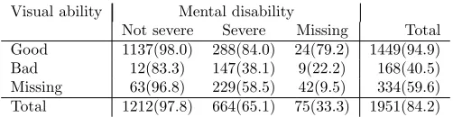
Visual ability Mental disability

Not severe Severe Missing Total

Good 1137(98.0) 288(84.0) 24(79.2) 1449(94.9)

Bad 12(83.3) 147(38.1) 9(22.2) 168(40.5)

Missing 63(96.8) 229(58.5) 42(9.5) 334(59.6)

Total 1212(97.8) 664(65.1) 75(33.3) 1951(84.2)

Table 2: Number and survival above age 21.5 of people with cerebral palsy: mental and

visual ability

drops significantly to 33.3%. Visual disability also appears to have a strong effect on

the survival. However, here bad vision has an even lower survival probability (40.5%)

than when the disability is missing (59.6%).

When both disabilities are missing, the survival probability is 9.5% and when both

disabilities are severe 38.1% (Table 1). It further appears that good or bad vision and

missing mental disability gives a worse probability of survival than vice versa. However, we also note that when an individual has bad vision, then he is also very likely to have a severe mental disability, while, given severe mental disability, the individuals are spread more evenly across the different categories of visual ability.

In the examples in later Sections of the paper we further omit four individuals who were censored before March 2011 and hence censored before having either died or reached the age of 21.5.

3

Chain Event Graphs

Chain Event Graphs (CEG) (Smith and Anderson 2008;Thwaites et al. 2010) generalise

the discrete Bayesian Network by allowing for context-specific conditional independen-cies, as well as providing a representation for the way in which different combinations of covariates can affect a variable of interest. CEGs are derived from a probability tree by merging the nodes whose edges describe the same succeeding event and whose associated conditional probabilities are the same. We define a CEG explicitly using the following

illustrative example based on the Mersey study introduced in Section2. Hence let Y1

describe the birth weight of the individual,Y2whether mental disability is severe or not

and letY3 indicate whether survival above the age of 21.5 is obtained.

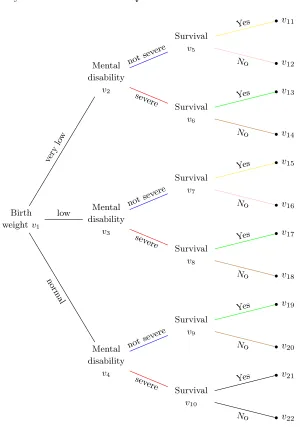
The corresponding event tree is given in Figure1.

We say that two non-leaf vertices,vi and vj, of the tree, T, are in the same stage, u,

when the edges emanating from the two vertices represent the same succeeding event so that we have a direct correspondence between their edge sets. Further, we require that

the conditional probabilities of the next event, given that one of the vertices in stageu

has been reached, are the same. We can therefore partition the vertices of the tree into

stages and we denote the set of all stages byJ(T). The stages containing more than

Birth weightv1

Mental disability

v4

Survival

v10

v22

No

v21

Yes sev

ere

Survival

v9

v20

No

v19

Yes

notsev ere normal

Mental disability

v3

Survival

v8

v18

No

v17

Yes sev

ere

Survival

v7

v16

No

v15

Yes

notsev ere

low

Mental disability

v2

Survival

v6

v14

No

v13

Yes sev

ere

Survival

v5

v12

No

v11

Yes

notsev ere

very low

Figure 1: Example of a tree,T, on three variables: birth weight, mental disability and

survival, with coloured stages

same colour. So, in this example, colouring of the tree gives the following set of stages:

u1={v1}, u2={v2, v3, v4}, u3={v5, v7}, u4={v6, v8, v9}, u5={v10}.

A finer partition of the stages of the tree is given by the definition of positions. We

such that we have a bijection between the edges of the two subtrees and the conditional

probabilities associated with the edges are the same. In our examplev5, v7andv6, v8, v9

are in the same position, as arev2, v3, whilev4 is in a separate position.

The CEG,C(T), is then the staged tree collapsed over its positions. Hence the vertices

of the graph are given by the positions of the tree with the leaf nodes of the tree being

collected in a single position, which we call w∞. Further, the edge set of the CEG

is defined as follows: Let v(w) be a representative vertex for positionw. Then there

exists an edge from a positionw to a positionw0 in the CEG for every edge from the

representative vertexv(w) to any vertexv∈w0. The stages of the tree are represented

in the CEG by connecting two positions that are in the same stage by an undirected

dotted line. For a formal definition seeSmith and Anderson(2008). In our example we

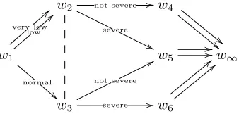
obtain the structure given in Figure2 with positions

w1={v1}, w2={v2, v3}, w3={v4}, w4={v5, v7}, w5={v6, v8, v9}, w6={v10}

w∞={v11, v12, v13, v14, v15, v16, v17, v18, v19, v20, v21, v22}.

w2 not severe //

severe

'

'

w4

"

""" w1

low

=

=

very low

=

=

normal

!

!

w5 ////w∞

w3 severe // not severe

7

7

w6

<

<

<

<

Figure 2: CEG derived from the tree,T

Given an event tree we may want to determine which nodes in the tree should be

merged to find the CEG structure which best fits a given data set. Freeman and

Smith(2011) demonstrated that all CEGs associated with a particular event tree can be scored according to the Bayesian Dirichlet metric, analogously to the scoring method

for Bayesian Networks developed inHeckerman et al. (1995)

Here we assume the natural prior independence of the vectors of conditional probabilities

associated with each stageu, Πu, corresponding to the local and global independence

assumption commonly used for inference in Bayesian Networks (seeCowell et al.(2007)).

We give each conditional probability vector Πu = (πu1, πu2, . . . , πuru) a prior Dirichlet

distribution with parameters (αu1, αu2, . . . , αuru), which takes the form

p(Πu|C(T)) =

Γ(αu) Qru

k=1Γ(αuk) ru

Y

k=1

παuk−1

uk ,

where αu=P

ru

k=1αuk andruis the number of edges emanating from stageu.

separately and in closed form resulting in the posterior distribution

p(Πu|D, C(T)) =

Γ(αu+Nu) Qru

k=1Γ(αuk+Nuk) ru

Y

k=1

παuk+Nuk−1

uk ,

where Nu =PkNuk and Nuk is the number of times we observe an individual going

from a vertex in stageuto a vertexk.

Freeman and Smith(2011) now follow an argument exactly analogous to that of Hecker-man et al.(1995) using ideas like parameter modularity to set up consistent priors over the parameters of each of the models in the selected trees. Thus as a default setting we often specify a uniform prior on the finest partition of the CEG such that every path that can be taken in the event tree is a priori equally likely. We further specify the

equivalent sample size,α=P

u∈J(T)αu, which determines the strength of the prior

be-lief, to be equal to the highest number of categories taken by a variable in the problem,

as suggested for Bayesian Networks in Neapolitan (2004). In our example, we hence

have α= 3. When two stages are merged then the parameters of the prior Dirichlet

distributions are deduced by summing the hyperparameters associated with the stages merged.

For simplicity, in this paper all possible CEG structures within a class of plausible models are given equal prior probability. In the simplest variants of our model search we can compare two models by calculating their associated Bayes Factor given by the ratio of their marginal likelihoods. The logarithm of the marginal likelihood of each CEG is then given by the linear score

logp(D|C(T)) = X

u∈J(T)

log Γ(αu)−log Γ(αu+Nu) +

ru

X

k=1

(log Γ(αuk+Nuk)−log Γ(αuk))

!

. (1)

Note that because this score function is additive and in closed form it is simple to evaluate. Furthermore, to calculate the Bayes Factor between two structures we only need to calculate the difference in score based on the stages in which they differ, as the

scores of all coinciding stages cancel. For more details on this approach see Freeman

and Smith (2011).

Usually the full space of CEG models is extremely large. This means that an exhaustive search across all possible CEG structures is only possible in the simplest cases. However, various numerical greedy search algorithms can be developed which exploit the linear form of the Bayes Factor score function. Perhaps the simplest is the Bayesian

Ag-glomerative Hierarchical Clustering (AHC) algorithm developed inFreeman and Smith

(2011). This starts with the finest partition of the CEG into stages, in which every

non-leaf node is in a separate stage and the leaf nodes are gathered in the positionw∞.

continues until the coarsest partition has been reached and then the CEG structure with the highest overall score is selected.

In many situations in medical or social sciences we have a binary response variable describing, for example, survival of a patient, the presence of a disease or the passing of an exam, and we want to determine which covariates affect this outcome variable. CEGs are a particularly useful tool to identify and visualise the different ways in which certain combinations of covariates affect the variable of interest. In this paper, we focus on a particular novel type of CEG, here called the ordinal CEG, which is restricted to problems with a binary outcome variable occurring last in the tree. It provides, in the above setting, a more easily interpretable graphical representation of the standard CEG by imposing a particular ordering on the positions of the graph.

Going back to the original tree in Figure1, let Y3 be our binary variable of interest,

describing survival up to the age of 21.5. We then first partition the non-leaf vertices

in the tree into vertex subsets, such that each subset consists of those vertices whose emanating edges describe the same succeeding event. Hence, according to the definition of the CEG, all vertices in a subset may be merged into positions or stages to obtain a plausible CEG structure. In our example, we therefore have the subsets

VY1 ={v1}, VY2 ={v2, v3, v4}, VY3 ={v5, v6, v7, v8, v9, v10}.

Note that each of the subsets is naturally associated with one of the variables in the

problem. Then, given a CEG structure,C(T), associated with the treeT, each vertex

subset can alternatively be partitioned into positions. We can hence write the vertex subsets of our example as follows:

VY1 ={w1}, VY2 ={w2, w3}, VY3={w4, w5, w6}.

The graph of the ordinal CEG then vertically aligns the positions forming a vertex subset.

Definition: LetTbe a tree onpvariables with a binary outcome variableYprepresented

by the leaf nodes in the tree. We say that a CEG, C(T), is an ordinal CEG with

respect toYp when the positions in each vertex subset associated with a variable Yi,

VYi, are vertically aligned in descending order with respect to the predictive probability

P(Yp= 0|D, C(T)).

If Yp describes survival as in our example, with Yp = 0 meaning that the individual

survives above the age of 21.5, the ordering occurs such that the position with the

highest probability of survival is at the top of the graph. This allows us to read off directly from the graph how the different combinations of covariates affect the survival probability: the higher up the graph a combination takes us the better the effect on the outcome variable. The ordinal CEG further retains the natural time ordering of the tree

by listing the vertex subsets fromY1 toYpfrom left to right in the graph. Note that in

Figure2, the CEG is written as an ordinal CEG. Each vertex subset,VYi, i = 2, .., p,

of the ordinal CEG hence defines a cut in the graph and we can look at each cut-set

outcome variable,Yp, at each point in time. This will be demonstrated in the example

in Section5.

In higher dimensional problems, the full ordinal CEG structure may become complicated when we have a large number of positions in each vertex subset. To improve the visual aspect of the ordinal CEG we can represent the graph as a reduced ordinal CEG. Here we restrict our interest entirely to the combined effect of the covariates on the

outcome variable by considering only the positions in the final subset, VYp, and

re-expressing the paths leading to these positions in terms of new variables. Hence only

the final subset of positions remains in the reduced ordinal CEG whileVY1 up toVYp−1

are redefined to describe simply the intermediate steps leading to the final subset of

positions. We represent these as intermediate positions, denoted by wI_{. We note that}

these intermediate positions do not necessarily follow the natural ordering in time. We

give a detailed example of this method in Section 6.

4

Missing Data and Models of Missingness

In many situations we cannot observe the full data matrix of a given problem. Many different reasons for missing values exist, including non-response due to the individual refusing to disclose information, censoring of observations due to death or migration, or simply loss of data. It is common practice to partition missing data mechanisms into three categories: Missing completely at random (MCAR), missing at random (MAR)

and missing not at random (MNAR) as proposed in Rubin (1976). The focus of this

paper will be to further partition the MNAR models.

To illustrate the application of the CEG to classify models of missingness, we apply this

representation to a subset of the Mersey study. Thus again let Y1 describe the birth

weight, Y2 the mental disability andY3 the variable describing the survival above the

age of 21.5. AsY3 is binary we can write the CEG as an ordinal CEG with respect to

the probability of survival and thus enhance the expressiveness of the graph. Also letY2

have missing values and letR2 be the variable indicating whetherY2is missing or not.

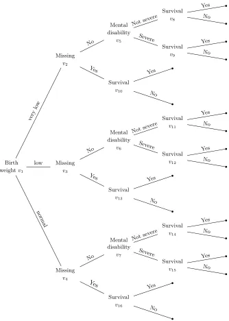
The corresponding event tree is given in Figure3. We slightly simplify the problem by

restricting the missingness only to the mental disability.

Because the CEG is derived from a tree we first choose a (partial) ordering of the variables. Ideally this order should be compatible with the temporal development of each unit within the study. Here, survival therefore represents the final variable in the tree as we are interested in the effect of the other two covariates on the probability of survival. Birth weight is introduced first, while mental disability, which is measured

later, is introduced second, giving the ordering of the variables: (Y1, R2, Y2, Y3). Unlike

Birth weightv1

Missing

v4

Survival

v16 _No

Yes

Yes

Mental disability

v7

Survival

v15 No

Yes Sev_ere

Survival

v14 No

Yes

Notsevere

No normal

Missing

v3

Survival

v13 _No

Yes Yes

Mental disability

v6

Survival

v12 No

Yes Sev_ere

Survival

v11 No

Yes

Notsevere

No

low

Missing

v2

Survival

v10 _No

Yes Yes

Mental disability

v5

Survival

v9 No

Yes Sev_ere

Survival

v8 No

Yes

Notsevere

No

very low

and differentiate various different MNAR structures explicitly. More precisely, we only

search over models which model the dependence of R2 with Y1 and Y2, as Y3 occurs

later within the tree. Similarly, in a larger example, we can look at the missingness mechanisms for different variables separately for each point in time across the cut-sets of the ordinal CEG.

As described in Section 3, the CEG allows us to merge any nodes in the tree whose

set of emanating edges describes the same succeeding event. Hence, in our example, according to the definition of the CEG, we can consider combining the vertices in each

of the vertex subsets,VR2,VY2 andVY3. When data are assumed to be MAR or MCAR

we observe a particular set of CEG structures which describe the randomness of the missingness mechanism. However, when data are MNAR, we can use the CEG structures to distinguish between hypotheses about different types of MNAR mechanisms, as we will illustrate below.

When data are MAR the missingness process is independent of the missing values given the observed values, so thatP(R2|Y1, Y2) =P(R2|Y1). This is identical to the assertion:

R2⊥⊥Y2|Y1.

Note that this implicitly takes the variables in the causal order (Y1, Y2, R2). In this

case the argument would be that the variablesY1 andY2 exist for each unit a priori,

however these variables might not be recorded for Y2 for various reasons. When this

censoring only depends onY1 then we have that data is MAR with respect toY2. We

note however that the assumption of MAR is probabilistically and statistically totally

equivalent to the assumptionY2 ⊥⊥R2|Y1. This reinterprets MAR in terms of viewing

data as if it were consistent with the causal order (Y1, R2, Y2). Here we assume that

Y1 and the missingness indicatorR2 can be seen as measurements of things happening

that might influenceY2. MAR then can be expressed as the equivalent requirement that

P(Y2|R2= 0, Y1) =P(Y2|R2= 1, Y1). Which of these two causal explanations of MAR

is most compelling is obviously dependent on context. For example if the data had already been collected and then some of the data lost, then the first causal mechanism would be most natural. If someone from the cohort left the study early before any outcome variable could be measured then the second causal ordering is most natural. Either way, if MAR is appropriate then, by the laws of probability, data will not allow us to distinguish between the two causal explanations: we can just choose the easiest and know the other is logically entailed. In this paper we choose the second causal ordering which allows models that violate the MAR assumption to still be estimated.

With respect to our example, under the assumption of MAR, we would expect v10 to

be in the stage whose predictive probability of survival is a weighted average of the predictive probabilities of survival for severe and not severe mental disability with very

low birth weight (v8, v9). The same holds for the vertices v13 and v16. However, note

that the MAR assumptions made need careful consideration. Here, we further imply

that the probability of survival is independent of the missingness process given Y1and

w2

missing

+

+

not missing //w₅ not severe // severe

w8

'

''' w1 bw low //

bw very low

7

7

bw normal

'

'

w3 missingnot missing //w6 11 severe

'

'

not severe

7

7

w9 //

/

/

w∞

w4

missing

3

3

not missing //w₇ severe // not severe

?

?

w10

7

7

7

7

Figure 4: Ordinal CEG when data are MAR

In this example we further have that survival is hypothesised to be independent of the birth weight given the visual ability and the missingness process. We assume that this holds throughout this Section for reasons of simplification. If this was not the case then

the positionsw8, w9andw10could be split into several positions depending on the birth

weight. As we are representing the graph as an ordinal CEG we are further assuming that a very low birth weight leads to the highest survival, followed by a low and normal

birth weight (Hutton and Pharoah 2002). For data to be MAR the position describing

the survival for the missing category must be in between the positions for survival of individuals with severe or non-severe mental impairment and in rare cases, when the disability categories are very imbalanced, then the missing category can coincide with the position of severe or non-severe mental disability respectively. However, this is only a necessary but not sufficient condition and so, to determine whether this means that data are likely to be MAR, it is necessary to additionally calculate the weighted average of the probability of survival and compare this with the true predictive probability of survival for the missing category. The graph on its own nevertheless gives an indication of the possibility that the MAR assumption holds. We will explore this in more detail in the next two Sections in which we carry out model selection on two examples.

If data are MCAR then the missingness process is independent of both the observed and the missing values, so that

R2⊥⊥Y1, Y2.

Hence in addition to the structure deduced for data that are MAR, i.e. R2 ⊥⊥Y2|Y1,

we can also represent thatR2 ⊥⊥Y1 directly through the graph. In our example this

requires that the vertices in subsetVY1 are merged into a stage such that the probability

of having a missing value is indistinguishable across birth weight. An example of this

is given in Figure5.

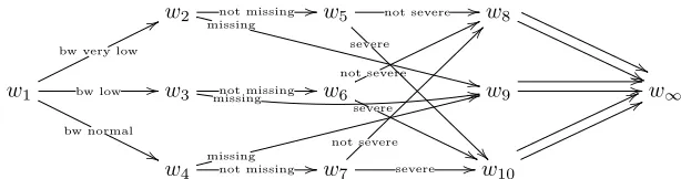
When data are MNAR then the missingness process depends on both the observed and

the unobserved values such thatR2 depends on bothY1 andY2. However, the ordinal

CEG can also represent different types of MNAR data and we describe several different cases below.

A simple case for MNAR occurs when all vertices describing that missingness has oc-curred are in positions with lower survival probability than when mental disability is

observed. In our example this means thatv10, v13 and v16 are in lower positions than

w2

missing

+

+

not missing //w₅ not severe // severe w8 ' ''' w1 bw low //

bw very low

7

7

bw normal

'

'

w3 missingnot missing //w6 11 severe ' ' not severe 7 7

w9 //

/ / w∞ w4 missing 3 3

not missing //w₇ severe // not severe ? ? w10 7 7 7 7

Figure 5: Ordinal CEG when data are MCAR

likely to be even worse than the usual mental disability which is classed as ‘severe’ or is associated with poorer survival. For example, we may have the ordinal CEG structure

given in Figure6. Here we can deduce directly from the graph alone that missingness

is unlikely to be MAR. As before, birth weight is hypothesised to be independent of

survival. We further note that ifw2, w3 andw4 were in the same stage, then we could

further deduce that the missingness indicator depends only on the missing values but not on the observed.

w2

missing

$

$

not missing //w₅ not severe // severe ' ' w8 ' ''' w1 bw low //

bw very low

7 7 bw normal ' ' w3 missing + +

not missing //w₆ severe // not severe

7

7

w9 ////w∞

w4 missingnot missing //w7 11 severe 7 7 not severe ? ? w10 7 7 7 7

Figure 6: Ordinal CEG when data are MNAR

Alternatively, we may have that data are MNAR conditional only on certain values of another variable. In our example, data may be MAR given that the birth weight is very low or low but MNAR when birth weight is normal. This hypothesis is represented by

the ordinal CEG with the structure given in Figure7. An extension of this could be a

model where we have two variables describing disabilities with missing values. Then we could further draw conclusions from the CEG distinguishing between data being MAR only with respect to certain variables.

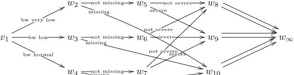
Further, the topology of the ordinal CEG is able to provide information on the potential distortion due to missingness. For example, we may have that when mental disability is missing then it is simply in the same position as an individual whose mental disability is

classed as ‘severe’, as illustrated in Figure8. However, when comparing this to Figure

6, then we see that the missing category has a stronger effect on survival in Figure 6

than in Figure8.

Finally, the opposite effect may be hypothesised, where the survival probability given that mental disability is missing is in the position with the highest probability of survival.

w2

missing

+

+

not missing //w₅ not severe // severe w8 ' ''' w1 bw low //

bw very low

7

7

bw normal

'

'

w3 missingnot missing //w6 11 severe ' ' not severe 7 7

w9 //

/ / w∞ w4 missing + +

not missing //w₇ severe // not severe ? ? w10 7 7 7 7 w11 > > > >

Figure 7: Ordinal CEG when data are MNAR conditional on birth weight

w2

missing

+

+

not missing //w₅ not severe // severe ' ' w8 ' ''' w1 bw low //

bw very low

7

7

bw normal

'

'

w3 missingnot missing //w6severe 11// not severe

7

7

w9 ////w∞

w4

missing

3

3

not missing //w₇

severe 7 7 not severe ? ?

Figure 8: Ordinal CEG when data are MNAR: potential distortion

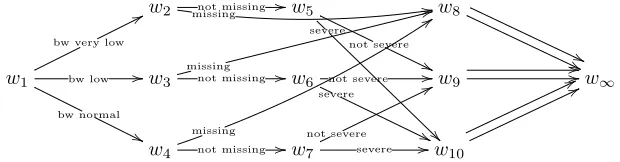
are MNAR, but now the conclusion made would be that missingness occurs only when the mental disability is non-severe. Of course an expert could deem such CEG structures and associated hypotheses implausible. However, these scenarios are simple to address within our methodology: we simply exclude models considered implausible by the expert from our search space, or alternatively assign them small prior probabilities and modify our score function accordingly. Note that such a methodology is fully consistent with the Bayesian paradigm where such prior domain knowledge is expressed explicitly within the inferential mechanism.

w2 missingnot missing //w5 11

not severe ' ' severe w8 ' ''' w1 bw low //

bw very low

7 7 bw normal ' ' w3 missing 3 3

not missing //w₆ severe

'

'

not severe //w₉ ////w_∞

w4

missing

:

:

not missing //w₇ severe // not severe 7 7 w10 7 7 7 7

Figure 9: Implausible ordinal CEG structure

in question. We have also illustrated that the ordinal CEG can distinguish between different types and patterns of MNAR and the way in which this is made explicit in the graph. In the next Section, we add the predictive probabilities of survival to each of the positions to enhance the inference that can be made from the graph.

We note that in our example missingness does not occur for the outcome variable. Nevertheless, this could also be incorporated into the CEG structure. In this case we would have an outcome variable with three categories, “survival”, “no survival” and “missing”, and we could add the predictive probabilities of survival and of missing survival to the graph, with the ordinal CEG being defined with respect to

P(Yp= 0|D, C(T)) as before.

5

Determining Missing Data Structures Through Model

Selection

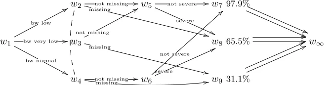
We next illustrate here the simple model selection methods applied to the example of the previous section to first determine through the structure of the CEG whether the data are likely to be MCAR, MAR or MNAR and further to obtain an understanding of the missingness structures beyond the three established mechanisms. Running the AHC algorithm on the Bayes Factor scores we find the most probable CEG for the

above problem on three variables, (Figure 10). We attach the posterior predictive

probabilities of survival above the age of 21.5 to the subsetVY3 in the CEG. These and

the 95% credible intervals of the posterior distribution of survival are: 97.9 (97.0,98.7)%

for position w7, 65.5 (61.8,69.1)% for w8 and 31.1 (19.8,43.8)% for w9. Note that we

again draw the CEG as an ordinal CEG such that the positions describing the same suceeding event are vertically aligned in descending order with respect to the predictive probability of survival.

w2

missing

+

+

not missing //w₅ not severe // severe

(

(

w797.9%

(

((( w1 bw very low //

bw low

8

8

bw normal

&

&

w3

missing

+

+

not missing

8

8

w865.5% ////w∞

w4 not missingmissing //w6 11 not severe

=

=

severe

6

6

w931.1%

6

6

6

6

Figure 10: Ordinal CEG on birth weight and mental disability

We can now draw a number of conclusions from the CEG about the likely dependence structure of the three variables considered. We can read that the distribution of the

missingness is indistinguishable for a low and normal birth weight as w2 and w4 are

in the same stage. Also, given a low or very low birth weight and given that mental disability is observed, we have that the distribution of mental disability and survival is

Note also from the topology of the ordinal CEG that a low birth weight gives the highest probability of survival followed by a very low and a normal birth weight. From position

w7 we can deduce that the highest probability of survival is obtained when mental

disability is observed to be non-severe. In this case survival above the age of 21.5 is

predicted to be 97.9%. When mental disability is observed to be severe, the individual

is forced into the final positionw8 with survival of 65.5%, which is significantly lower

than survival with a non-severe disability. In both cases we further have that survival is independent of birth weight given mental disability. The poorest survival is found to be for individuals whose mental disability is not observed. Here a low birth weight leads to a predicted survival equal to the predicted survival for severe disability, while

for a very low or normal birth weight survival is predicted to be only 31.1%. This is

much lower than survival when mental disability is observed and hence we can deduce directly from the ordinal CEG structure that the data are unlikely to be MAR.

We can further derive the expected survival probabilities for individuals for whom men-tal disability is missing under various assumptions. If we assume that the data are MAR then we would expect the survival probability conditional on a particular birth weight to be the average of the survival probability for individuals of that birth weight with a severe or non-severe disability, weighted according to the proportion of individuals with severe or non-severe mental impairment. Hence an individual with a very low weight at

birth has a survival probability of 97.9×(166/224) + 65.5×(58/224) = 89.5% past the

age of 21.5, where 166 individuals have very low birth weight and no severe disability

and 58 individuals have very low birth weight and a severe disability. Similarly the

ex-pected percentages for a low or normal birth weight are 87.7% and 85.4%, respectively.

However, we see that the edges describing the missingness lead to positions w8 and

w9 whose predictive probabilities of survival are much lower, namely 65.5% and 31.1%.

Therefore the data are unlikely to be MAR. In the situation where the individual has a very low or normal birth weight we can read this off directly from the ordinal CEG. For a low birth weight, the missing edge leads to the same position as severe mental

disability with survival probability 65.5%.

Figure 10suggests that the data are not MAR, however the weighted average needs to

be calculated to make reliable conclusions, since if the proportion of individuals with non severe mental disability was very small, then MAR data could still merge severe and missing mental disability into the same position. Nevertheless, the ordinal CEG gives a good primary overview of the missingness structure and the plausibility of the data being MAR or not.

When carrying out model selection on the tree given in Figure 3 we can also examine

the hypothesis that the data are MCAR. The first requirement for this is that w2, w3

andw4are in the same stage, which suggests that there is no evidence that missingness

is dependent on the birth weight of the child. However, this is only the case forw2and

w4 but not forw3. The second requirement, that missingness is independent of mental

disability, does also not appear to be plausible, because of the reasons given above.

We finally note how the ordinal CEG allows us to discuss different types of missingness

ordinal CEG. Hence we can read from the first cut-set that missingness is dependent on the birth weight of the child, though indistinguishable for a low and normal birth weight. From the second cut-set we can deduce that mental disability is dependent on the birth weight of the child and finally, from the third that survival depends not only on mental disability but also on the missingness process.

6

An Example on Four Variables

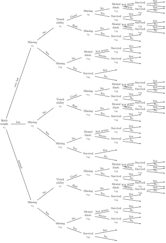
In this Section we demonstrate how the methods above can be simply extended to obtain a more nuanced analysis of a data set. We extend our model space by including a further variable into our model describing visual ability. We choose an ordering such that birth weight occurs first, followed by visual ability and then mental disability. The

final variable in the tree is again survival above the age of 21.5, the variable of interest.

The corresponding tree structure of this extended problem is given in Figure11.

We can again find the most probable CEG structure for this problem, given in Figure

13 in the appendix, using the AHC algorithm described in Section 3. However, the

resulting CEG structure is complicated such that it cannot be easily read by a client.

More explicitly, the nodes v2 up to v25 are often only merged into stages but not

positions, so that in the resulting CEG structure we have up to nine positions in one subset with 18 edges emerging from them leading to seven positions of the next subset. We therefore consider an alternative representation using a reduced ordinal CEG.

One plausible simplification of Figure13can be found by defining the variable ‘number

of severe disabilities’ with six categories: no disability, one disability non-severe and one missing, exactly one disability severe, one disability severe and one missing, two

disabilities severe and both disabilities missing (Hutton et al. 1994). The corresponding

new illustration is given in Figure12. The number of disabilities appears first in the

graph. When both disabilities are missing we distinguish between low birth weight or not low birth weight. Given that one disability is missing we identify the type of disability that is observed, to distinguish between different positions. Finally, when exactly one disability is severe, we first distinguish between a low birth weight or not, and in the case of a low birth weight whether visual or mental disability is observed to

be severe. Note that positionswI

2 up towI6 are intermediate positions describing only

an intermediate step in the paths of the individuals in reaching the final positions. For

example, it may be thatwI

2, w4I andwI3, w5I are in the same stage, however this is not

known from model selection on the original tree. Also, birth weight occurs after the number of disabilities, hence not following the ordering in time of the tree.

We further note that there are four paths to survival which do not comply with this

CEG and whose final edges are marked in red in Figure13. The paths are the

follow-ing: individuals with very low or low birth weight, bad vision and non-severe mental disability; individuals with low birth weight, good visual ability and missing mental dis-ability; individuals with normal birth weight, bad vision and missing mental disability.

However, these paths are only taken by one or two individuals (see Table2) and hence

Birth weight v1 Missing v4 Missing v16 Survival

v52 No

Yes Yes

Mental disab.

v25 Survival

v51 No

Yes Severe

Survival

v50 No

Yes Not severe

No Yes Visual ability v7 Missing v15 Survival

v49 No

Yes Yes Mental disab. v24 Survival v48 No Yes Severe Survival v47 No Yes Not severe No Bad Missing v14 Survival

v46 No

Yes Yes Mental disab. v23 Survival v45 No Yes Severe Survival v44 No Yes Not severe No Good No normal Missing v3 Missing v13 Survival

v43 No

Yes Yes

Mental disab.

v22 Survival

v42 No

Yes Severe

Survival

v41 No

Yes Not severe

No Yes Visual ability v6 Missing v12 Survival

v40 No

Yes Yes Mental disab. v21 Survival v39 No Yes Severe Survival v38 No Yes Not severe No Bad Missing v11 Survival

v37 No

Yes Yes Mental disab. v20 Survival v36 No Yes Severe Survival v35 No Yes Not severe No Good No low Missing v2 Missing v10 Survival

v34 No

Yes Yes

Mental disab.

v19 Survival

v33 No

Yes Severe

Survival

v32 No

Yes Not severe

No Yes Visual ability v5 Missing v9 Survival

v31 No

Yes Yes Mental disab. v18 Survival v30 No Yes Severe Survival v29 No Yes Not severe No Bad Missing v8 Survival

v28 No

Yes Yes Mental disab. v17 Survival v27 No Yes Severe Survival v26 No Yes Not severe No Good No very low

from the AHC algorithm and the CEG for which the four paths are put into positions

compatible with the new representation is 2.97 and hence we can conclude that our

simplified representation is only slightly less favoured than the CEG found through the algorithm.

wI

2 mental observed //

visual observed

+

+

w797.9%

$

$$$

wI

6

mental severe

6

6

bad vision

(

(

w1

0+miss

A

A

1 disability //

0 disability

'

'

1+ miss

&

&

2 disabilities

1

1

2 missing

wI

3 bw very low ,normal //

bw low

5

5

w882.6% ////w∞

wI₄ mental observed //

visual observed

,

,

w958.8%

4

4

4

4

w1037.1%

:

:

:

:

wI₅ bw very low, normal //

bw low

2

2

w11 0.4%

?

?

?

?

Figure 12: Reduced ordinal CEG on birth weight and visual and mental disability

The percentages attached to the five final positions in Figure 12 give the posterior

predictive percentages of survival given an individual reaches that position. We have

the following percentages and 95% credible intervals: 97.9 (97.0,98.6)% for position

w7, 82.6 (77.8,86.9)% forw8, 58.8 (52.3,65.2)% forw9, 37.1 (29.7,44.8)% for w10 and

0.4 (0,3.6)% forw11. We see that we have the poorest survival when both disabilities

are missing and the birth weight is either very low or normal. When birth weight is

low, then the predictive probability of survival is still as low as 37.1% which is equal

to the survival when both disabilties are observed to be severe. When one disability is severe and the other is missing then survival splits according to which disability is observed. The graph suggests that survival is lower when visual disability is observed than when mental disability is observed. In the former case the probability of survival is indistinguishable from the case where both disabilities are severe as both paths lead

to positionw10. For either disability we observe that the probability of survival appears

to be lower than when exactly one disability is present. Moving further up the graph we see that when exactly one disability is observed to be severe, then the predictive survival

this depends on whether the birth weight is low or not and whether the visual or mental disability is severe. When one disability is non-severe and the other is missing we reach

the same two positions, w7 and w8, and survival again depends on which disability is

observed, with visual disability observed resulting in the lower position. Finally survival is best when both disabilities are observed to be non-severe.

Probability of survival in %

Expected under MAR Predictive

No disability+1 missing 95.3 93.7

Mental disability observed 97.7 97.9

Visual ability observed 95.4 82.6

1 disability+1 missing 69.9 58.0

Mental disability observed 69.5 58.8

Visual ability observed 40.7 37.1

Both missing 90.0 3.7

Table 3: Plausibility of MAR assumption for disability in cerebral palsy survival

We can further deduce directly from the topology of the reduced ordinal CEG that data are highly unlikely to be MAR when both disabilities are missing, as survival, once

w11 has been reached, is significantly lower than survival for the other positions. In

Table3we calculate the expected probabilities of survival under the MAR assumptions

as in Section4 by taking a weighted average of the predictive probabilities of survival

weighted according to the proportion of individuals going along the different possible paths. Again careful consideration of the MAR assumptions is needed. These will be discussed for several variables with missing values in a later paper.

Table3shows that the expected probability of survival when both variables are missing

is 90%,the weighted average of the survival of people with two disabilities, exactly one

disability and no disabilities. In contrast to this the predictive probability of survival for

this data set is 3.7% (a weighted average of 37.1% and 0.4%), which strongly supports

the hypothesis that data are not MAR.

Given that one disability is observed to be severe and the other is missing, data again appear unlikely to be MAR as the individuals considered have predictive probabilities

of survival of 58.8% and 37.1% which are noticeably lower than individuals with exactly

one disability. Table3 again supports this hypothesis since the expected probability of

survival is 69.9% versus 58% for the predictive probability. The table provides evidence

that when the visual disability is measured then data are likely to be MAR (40.7%

versus 37.1%). We here refer back to Table 2which shows that when an individual has

bad vision, then mental disability is predominantly severe, while few individuals have bad vision and non-severe mental disability. Hence the calculated weighted average is very close to the probability of survival for the two disability case. In contrast to this we have that data are unlikely to be MAR when the mental disability is observed, with

the predictive probability of survival being significantly lower at 58.8% while we would

When one disability is non-severe and the other is missing then the table suggests that

data may be MAR as the predictive probability of survival is, at 93.7%, only slightly

lower than what we would expect under the MAR assumption. The graph illustrates this hypothesis since individuals with one non-severe disability and the other missing split between the positions describing no disabilities and exactly one disability. Given that we know which disability is observed, we have the reverse to the previous case: data are unlikely to be MAR when visual ability is observed and likely to be MAR when mental disability is observed.

7

Conclusions

We believe that the methods developed in this paper provide a useful new way of exploring certain classes of models systematically for evidence of various different types of MNAR hypotheses as well as investigating the plausibility of the MAR assumption within these models. The graph of the ordinal CEG enables us to obtain a precise understanding of the subtleties associated with the three common types of missingness and differentiate further between more refined MNAR structures. Whilst not MAR these structures still have sufficient symmetries to be efficiently estimated and scored using standard Bayes Factor techniques. In some studies, there can be different reasons for missingness. In our example we might be able to distinguish between missingness due to the impossibility of measuring the disability and missingness due to non-response or loss to follow-up. A missingness indicator can have more than two categories, or be represented with two variables, the first for missingness and the second giving the reason for missingness. This is simply modelled within a CEG. However, the meaning and hence the assumptions of MAR when we have two missingness indicators will require context-specific discussion and definition.

Of course these models are not universally acceptable. In particular they require contex-tual meaning for certain orderings of the variables that lead to a tree. Such information is not always available, although we find in many examples we have studied, like the one in this paper, that it is. We note that if there are several different interpretable trees we can in principle simply extend the model space to include CEGs associated

with trees expressing different orderings. Alternatively, as demonstrated in Section6,

we can restrict our search to only a subset of vertices in the tree, for example, if we are interested in the way a combination of variables affect a set of variables which occur later in time, and represent the graph as a reduced ordinal CEG.

We further believe that elicitation techniques as used for Bayesian Networks can be usefully applied to CEGs. The explanation of a process is then elicited from a client. For large scale problems the Bayesian statistician can then zoom into parts of the resulting CEG structure to show to the client. In particular, the statistician can further feed back possible reduced ordinal CEG structures to the client and investigate the plausibility of these reductions, which become apparent through the MAP CEG structure, with the client.

is extremely large. To investigate the robustness of the MAP model it may be of interest to carry out an exhaustive search of models close to the MAP model found by the AHC algorithm. More sophisticated model search methods, such as the weighted MAX-SAT

algorithm for Bayesian Networks (Cussens 2008) need to be developed for CEGs if

our methods are to be fully exploited for large scale problems. A further alternative would be to use CEGs in large problems represented by a Bayesian Network by finding the MAP CEG structure for a subset of variables in the BN. This would allow for a compact representation, however, with a detailed account of the missing data structures as presented in the paper. Such models are currently being investigated.

Appendix

Figure13shows the original CEG structure obtained from the tree in Figure11using

the AHC algorithm. Note thatw24 corresponds to w7 in Figure 12and similarly w25

corresponds tow8, w26 to w9, w27 to w10 and finally, w28 to w11. The edges marked

in red represent the four paths taken by only one or two individuals, which are not

compatible with the representation in Figure 12.

w2 not miss miss # # w5 good vision ' ' bad vision

w8 not miss // miss , , w17 non-severe * * severe * *

w9 not miss // miss

,

,

w18 non severe // severe

*

*

w24

w10 _missnot miss //w₁₉ 11

non-severe

4

4

severe //_w25

'

'''

w1 bw very low // bw low D D bw normal w3 not miss D D miss ' ' w6 good vision D D bad vision

w11 not miss // miss

,

,

w20 severe //

non-severe

:

:

w26 ////w∞

w12 not miss 7 7 miss " " w21 non-severe ? ?

severe //_w27

7 7 7 7 w13 miss & & not miss > > w22 non-severe ? ? severe 4 4

w4 not miss // miss 7 7 w7 good vision G G bad vision ' ' w14 not miss > > miss 5 5 w23 non-severe : : severe : : w15 not miss > > miss , , w16 not miss > > miss < < w28 H H H H

Figure 13: Ordinal CEG on birth weight and visual and mental ability

References

M. Akacha and N. Benda. The impact of dropouts on the analysis of dose-finding studies

L.M. Barclay, J.L. Hutton, and J.Q. Smith. Refining a Bayesian Network using a

Chain Event Graph. International Journal of Approximate Reasoning, 2013. doi:

10.1016/j.ijar.2013.05.006. 54

J. Copas. What works?: selectivity models and meta-analysis. Journal of the Royal

Statistical Society: Series A (Statistics in Society), 162(1):95–109, 1999. 53

J.B. Copas and JQ Shi. Reanalysis of epidemiological evidence on lung cancer and

passive smoking. British Medical Journal, 320(7232):417–418, 2000. 53

R.G. Cowell, A.P. Dawid, S.L. Lauritzen, and D.J. Spiegelhalter.Probabilistic Networks

and Expert Systems. Springer Verlag, 2007. 58

J. Cussens. Bayesian network learning by compiling to weighted max-sat. InProceedings

of the 24th Conference on Uncertainty in Artificial Intelligence (UAI 2008), pages

105–112, 2008. 74

G. Freeman and J.Q. Smith. Bayesian map model selection of chain event graphs.

Journal of Multivariate Analysis, 102(7):1152–1165, 2011. 54,58,59

D. Heckerman, D. Geiger, and D.M. Chickering. Learning bayesian networks: The

combination of knowledge and statistical data. Machine learning, 20(3):197–243,

1995. 58,59

JL Hutton and POD Pharoah. Effects of cognitive, motor, and sensory disabilities on

survival in cerebral palsy. Archives of disease in Childhood, 86(2):84–89, 2002. 55,64

J.L. Hutton, T. Cooke, and P.O.D. Pharoah. Life expectancy in children with cerebral

palsy. British Medical Journal, 309(6952):431–435, 1994. 69

R.J.A. Little and D.B. Rubin. Statistical Analysis with Missing Data. Wiley, 2002. 53

R.E. Neapolitan. Learning Bayesian Networks. Pearson Prentice Hall Upper Saddle

River, NJ, 2004. 59

D.B. Rubin. Inference and missing data. Biometrika, 63(3):581–592, 1976. 61

J.L. Schafer. Analysis of incomplete multivariate data, volume 72. Chapman &

Hall/CRC, 1997. 53

J.Q. Smith and P.E. Anderson. Conditional independence and chain event graphs.

Artificial Intelligence, 172(1):42–68, 2008. 54,56,58

J.A.C. Sterne, I.R. White, J.B. Carlin, M. Spratt, P. Royston, M.G. Kenward, A.M. Wood, and J.R. Carpenter. Multiple imputation for missing data in epidemiological

and clinical research: potential and pitfalls. British Medical Journal, 338:157–160,

2009. 53

P. Thwaites, J.Q. Smith, and E. Riccomagno. Causal analysis with chain event graphs.

C. Winship, R.D. Mare, and J.R. Warren. Latent Class Models for contingency tables

with missing data. In Jacques A Hagenaars and Allan L McCutcheon, editors,Applied

Latent Class Analysis, pages 408–432. Cambridge University Press, 2002. 54

Acknowledgments